國 立 交 通 大 學
經營管理研究所
博 士 論 文
No.140
下游廠商領導之供應鏈體系的賽局分析
A Game-Theoretic Analysis of the Downstream Firm-Led
Supply Chain
研 究 生: 韓 宗 甫
指導教授: 胡 均 立 教授
下游廠商領導之供應鏈體系的賽局分析
A Game-Theoretic Analysis of the Downstream Firm-Led Supply Chain
研 究 生:韓宗甫 Student:Tsung-Fu Han
指導教授:胡均立 Advisor:Dr. Jin-Li Hu
國立交通大學
經營管理研究所
博士論文
A DissertationSubmitted to Institute of Business and Management College of Management
National Chiao Tung University in Partial Fulfillment of the Requirements
for the Degree of Doctor of Philosophy
in
Business and Management
July 2011
Taipei, Taiwan, Republic of China
下游廠商領導之供應鏈體系的賽局分析
研究生:韓宗甫 指導教授:胡均立 教授
國立交通大學經營管理研究所博士班
摘 要
供應鏈體系中有愈來愈多的現象顯示,處於下游的零售商逐漸在供應鏈的環節中扮 演愈來愈強勢的角色。在本研究中,即考慮在具有此一情況下,應用賽局理論之互動架構 發展供應鏈模型,以探討供應鏈成員間之決策行為。本研究以二階層供應鏈模型為基本架 構,成員包含上游兩家生產類似產品,相互具有替代性之製造商,而下游為單一零售商。 所發展出四個二階層供應鏈模型,第一個模型為上游製造商同時且各自對零售商所採行之 決策進行反應;第二個模型為上游兩製造商間採取勾結以回應零售商之所採取之行動;第 三個模型為上游兩製造商間具有領導廠商與追隨廠商之互動架構下,回應零售商之所採取 之行動。以上三個模型皆是以零售商應先行決策下所形成之供應鏈模型。而第四個模型則 是以供應鏈上游成員先行決策之角度出發,下游成員再跟隨反應之情況,作為與前三個模 型之對照。藉由調整上游兩製造商間所生產產品之替代性、生產成本、需求大小及彈性, 所得到之數值分析結果為: (1)身為供應鏈體系下之領導者,零售商所獲得之利潤高於上游 兩製造商。(2)若上游製造商間存在有勾結時,其可從下游零售商手中贏回部份利益,但下 游零售商仍握有大部分利益。(3)當上游製造商間存在領導廠商與追隨廠商情形時,上游廠 商利潤提升,且領導廠商獲利程度有可能優於下游零售商。(4)當上下游先行角色互換後, 其供應鏈上下游間成員利益之分配明顯逆轉。(5)在下游廠商領導情況下,生產者剩餘以上游廠商間勾結之情況為最大,消費者剩餘與福利則以上游廠商處於競爭情況下為最大。 關鍵詞:二階層供應鏈模型、賽局理論、下游廠商領導
A Game-Theoretic Analysis of the Downstream Firm-Led Supply Chain
Student: Tsung-Fu Han Advisor: Dr. Jin-Li Hu
Institute of Business and Management
National Chiao Tung University
Abstract
Some evidence appears the downstream retailer plays a dominant role in the supply chain. This study applies a game-theoretic interactive mechanism to analyze the leading effects in a supply chain. The setting of the two-echelon supply chain in our study comprises two members (manufacturers or vendors) in the upstream, which produce their products with some extent of substitutability, and one member (retailer) in downstream. Four interactive models based on game theory are developed: The first model assumes that upstream members are independent and simultaneous to react to the retailer’s decision. The second model represents these two upstream members taking up collusion to respond the downstream action. The third model applies the leader-follower interactive mechanism between the upstream members. The three models above are under the downstream firm-led situation in the supply chain. The fourth model reverses the setting that upstream members act as the leader, which will be contrast with the previous three downstream firm-led models. All these models’ solution processes are applied by backward induction approach of game theory. By applying some numerical examples with different scenarios, there are some findings: (i) As the downstream leader in the supply chain, the retailer gains profit more than the upstream manufacturers. (ii) If the
duopolistic manufacturers act in union, they can take back a little of benefits from downstream retailer, however, the downstream member still owns the biggest share of profit. (iii) Applying leader-follower interactive mechanism between upstream members improves their profits, the leader manufacturer may outperform downstream retailer in profit under some condition. (iv) There is drastic change in profit distribution as the leader-follower roles redirection between the downstream and upstream members. (v) Among the downstream firm-led models, consumer surplus and welfare exhibit identical order across cases: Upstream members’ competition facilitates the best welfare, collusion leads to the worst welfare.
Acknowledgement
I would like to express my sincerest gratitude to my advisor, Dr. Jin-Li Hu, for his patient guidance and direction during my doctoral program. He not only leads me in academic research, but a mentor inspires me all the time. Words are inadequate to express my thanks to him.
I extend my appreciation to the committee members, including Professor Mei-Fang Chen, Professor Chih-Hua Chiao, Professor Jiunn-Rong Chiou, Professor Yi-Kuei Lin, Professor Fang-Tai Tseng and Professor Chyan Yang, for their valuable suggestions and comments in my oral defense which have strengthened this dissertation and future research. In addition, many thanks are given to Professor Cherng G. Ding, Professor Edwin Tang, Professor Ray-Yeutien Chou and Professor Chieh-Peng Lin for providing detailed instructions during the research process. I am also grateful to Ms. Hsiao for her considerate helps through the routines of graduate studies.
Meanwhile, I wish to show my gratitude to my colleagues at TNU for their friendship and kindness during my Ph.D. study. I also offer my regards and blessings to all of those who supported me in any respect during the completion of the dissertation. Finally, I am heartily thankful to my family members, especially my wife and lovely daughter, for their love, support and encouragement. This work is dedicated to all of you.
Table of Contents
摘 要 ... i
Abstract... iii
Acknowledgement ... v
Table of Contents... vi
List of Figures... viii
List of Tables ... ix
Chapter 1 Introduction... 1
1.1 Research Background ... 1
1.2 Research Purpose... 5
1.3 Organization of the Dissertation... 7
Chapter 2 Literature Review ... 9
2.1 Introduction to Game Theory ... 9
2.1.1 Cournot Model... 13
2.1.2 Stackelberg Model ... 14
2.2 Application of Game Theory in Supply Chain Models ... 15
Chapter 3 The Two-Echelon Supply Chain Models ... 24
3.1 Model of Upstream Members Reacting Simultaneously and Independently (R-S Model) ... 26
3.2 Model of Upstream Members Acting in Collusion (C-S Model) ... 28
3.3 Model of Upstream Members in a Leader-Follower Structure (L-F Model) ... 30
3.4 Model of Upstream Members in Domination (M-D Model)... 31
4.1 Two Identical Demand Functions... 34
4.2 Discrepancy in Market Demand ... 37
4.3 Discrepancy in Manufacturing Cost ... 40
4.4 Discrepancy in Demand Elasticity ... 43
4.5 Welfare Distribution across Four Cases ... 46
Chapter 5 Concluding Remarks... 48
References ... 52
Appendix A. Analytical Solutions of L-F Model ... 58
List of Figures
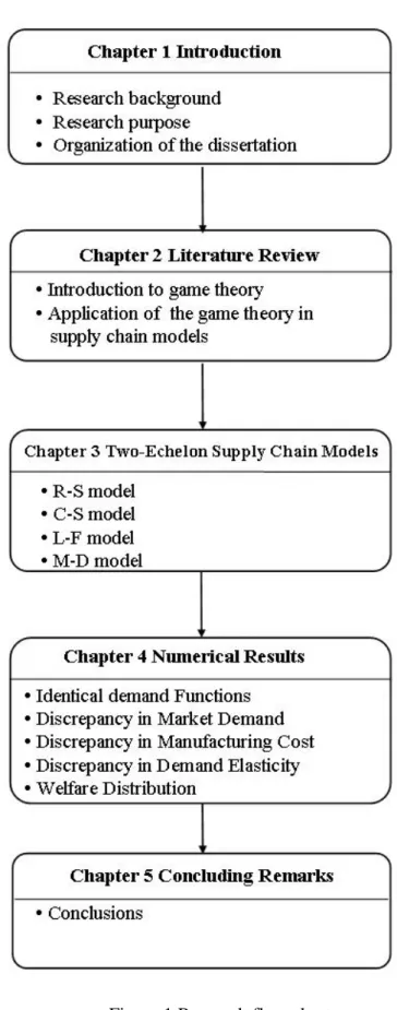
Figure 1 Research flow chart………8
Figure 2 The normal form of “prisoner’s dilemma”……...………10
Figure 3 The extensive form of “prisoner’s dilemma”…………..……….11
List of Tables
Table 1 Summary of the supply chain model literatures..………..22
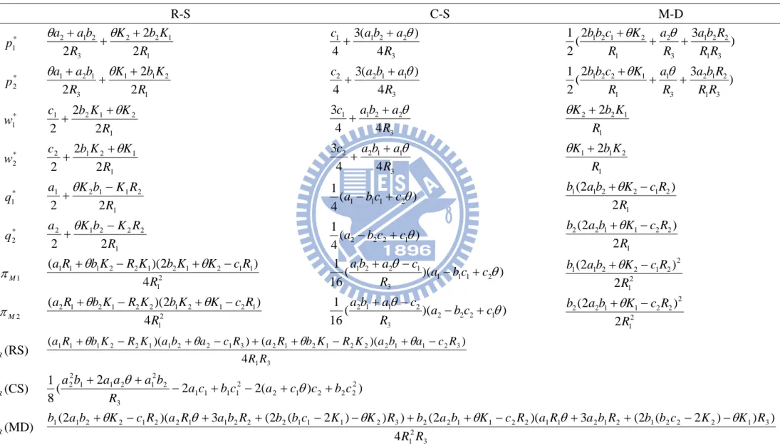
Table 2 Analytical solutions of the two-echelon supply chain models………...33
Table 3 Numerical results that two upstream firms are identical………...………36
Table 4 Numerical results of the different market demand……….………..39
Table 5 Variation of the solutions (in percentage) as manufacturer 1’s demand increasing 50%..40
Table 6 Numerical results of the different manufacturing cost………..…………42
Table 7 Variation of the solutions (in percentage) as manufacturer 2’s cost increasing 50%...43
Table 8 Numerical results of the different demand elasticity……….………45
Table 9 Variation of the solutions (in percentage) as manufacturer 2’s demand elasticity increasing 50%...46
Chapter 1 Introduction
1.1 Research Background
In the first half of 1900s, the enterprises faced a slow-moving market. Most of the industry’s upstream and downstream members operate individually, market information pass from downstream marketplace to upstream members tardily. Therefore, there exists a lag to the suppliers in responding market demand. Some manufacturers attempt to fully control much of their upstream resources and downstream sale channels. Take Ford motor company for example, it owned and operated iron mines, steel mills, farms, sawmills, parts plants, car assembly plants and retail showroom. From the raw materials to finished products, Ford motor company took part in every stage of the production activities. This is also known as vertical integration, to gain maximum efficiency through economies of scale (Betz, 2003). Today, rapid pace of technological progress forces organizations to face highly competitive markets. In the fast-moving markets of present economy, companies are required to have more flexibility and responsiveness. As organization grows bigger, globalization becomes inevitable for some reasons such as resources availability and market accessibility. It would be far beyond the control for enterprises to involve in every stage of manufacturing, distributing and marketing. A company’s competitive strategy defines the set of customer needs that it seeks to satisfy through its products or services. In order to fulfill the customer’s request, it will be a better way for different companies to work through the whole process and every one of them focuses on their ‘core competence’ and outsources the rest.
Supply chain represents product moves from supplies to manufacturers to distributors to retailers to customers along a chain (Chopra and Meindl, 2001). Ayers (2001) defines supply chain management as: “Life cycle processes comprising physical, information, financial, and
knowledge flows whose purpose is to satisfy end-user requirements with products and services from multiple linked suppliers.” The primary purpose for the existence of supply chain is to fulfill various customers’ needs. In any given supply chain, there are some combinations of enterprises that perform different functions, such as manufacturers, distributors or wholesalers, retailers. However, the fact is that market demands fluctuate all the time. As market demand changes, the upstream supply chain members would suffer the so-called ‘bullwhip’ effect. The more upstream they are, the more impacts they face. Nevertheless, supply chain members concern about their own benefits, even some of them are conflict each other. Promising high service levels to customers would cause over inventory, meanwhile, such action would increase holding costs and decrease operating efficiency. It is necessary to take a system approach to understand and coordinate the different member’s activities. The system approach that provides the framework to coordinate the flow of products and services to best serve the end customers is so-called supply chain management.
Supply chain management arouse in the late 1980s and widespread in the 1990s. Business used term such as “logistics” before that time. There are distinct differences between the concepts of supply chain management and traditional logistics. Traditional logistics focus on activities such as procurement, distribution, and inventory management. Supply chain management embraces all of the traditional logistics, but adds activities such as marketing, product development, finance, and customer service. The main idea of the supply chain management is to employ a systematic framework, integrating the upstream and downstream members in the industry by common goals and shared information, to lessen the lead time of production and respond the market demand promptly. The goal of supply chain management is to facilitate high throughput while simultaneously reducing both inventory and operating
expenses, keeping overall supply chain profitability. Ballou et al. (2000) has mentioned the coordination is a central lever of supply chain management. Li and Zhang (2008) also emphasize information sharing helps to improve supply chain profits.
As globalization and multinational corporations emerge, supply chain management are widely adopted by managers and applied in diverse industries. Johnson (2006) points out globalization and technology continually presented the world with new supply chain challenges and opportunities for further progress.
Studies in supply chain have demonstrated that in many industries retailers have increased their power relative to the manufacturer’s power over the last two decades (Messinger and Narasimhan, 1995). Manufacturers that had dominated their retailers in the past are finding that many retailers now hold the upper hand. In the past, the Procter and Gamble company (P&G) would act as the leader and dictate to their downstream retailer such as Wal-Mart. P&G’s decides what products would sell to Wal-Mart at what prices and under what terms. Besides, P&G used to limit the quantities of high demand products they would deliver to Wal-Mart, insist that Wal-Mart carry all sizes of a certain product, and asks that Wal-Mart participate in promotional programs.
But the situation somehow seems to be different (Li et al., 2002). Some retailers have grown to the point where the revenues are many times than their upstream supply chain members. Now, Wal-Mart, the retailer giant running over 9,000 stores across 15 countries with a remarkable revenue record of U$405 billion in 2010, is the most famous retailer reaching and retaining its success by a totally price reduction policy (Hesterly, 2010). In order to keep its promise to customers, Wal-Mart’s competitive strategy and supply chain strategy must fit together. Wal-Mart owns the superiority to bargain with its suppliers. Retailers, with the enormous scale
relative to their upstream suppliers, would require the suppliers to coordinate in related operations, such as inventory level, quantity discount, advertisement, terms of payment, or slotting fees. If the products do not sell well as expected, the suppliers will face the threat of moving products to poor shelf location or even to be dropped. Some suppliers who are lured by the big volumes to deal with Wal-Mart, but there are even cases that some suppliers eventually have no choice to disconnect with Wal-Mart for they can not keep the pace with the low price strategy (Norman, 2004).
Wal-Mart has strong impacts on a community and country in many wide aspects. Hicks (2006) concludes the so-called Wal-Mart effect in 3 types: (1) The income effect states that the lower retail prices may allow consumers to increase purchases, hence leading to higher employment and income in the retailer sector. Goetz and Swaminathan (2006) indicate that there exists a statistically significant increase effect of each Wal-Mart store on the United States’ countywide family-poverty rate with an average of 0.099%. However, a smaller reduction in the family-poverty rate, which might possibly be derived from the policy of minimizing the worker’s wage, is also found in places that had no stores. The estimate of the overall income effect must offset the above two effects. (2) The cluster effect refers to the geographic firm network naturally formed to share a common labor market, transportation, and the technologies of Wal-Mart, which bring a net increase of employment, wages, and firms as a consequence. (3) The productivity effect refers to the overall economic growth resulting from the new inputs (more workers, more natural resources, and more machinery) and the more intensive production process for workers to produce more goods or services with the same inputs. It is found that Wal-Mart’s price policy does not remain only in its store, but spills over to bring domestic retail prices down in the product markets it enters. Basker (2005) shows evidence that price decline is
economically large, 1.5-3.0%, in the short run and four times as much in the long run and is statistically significant.
Since the supply chain members’ power has shifted from upstream to downstream to certain extent, it would be interesting to survey how the impact to the supply chain member’s benefits. Whether the supply chain operates more efficient or customers gain the benefits from the change under the downstream firm-led structure are explored. In this study, we are going to discuss the supply chain in the game theoretic view.
1.2 Research Purpose
Every member in the supply chain needs to earn his profit to sustain operations. Take a three-echelon supply chain for example, the upstream manufacturers organize the raw materials or components and make/assemble them into finished goods. With the direct costs plus margin, the products are sold to the wholesalers. The wholesalers then distribute products to the retailers with necessary markup. Finally, the retailers set the retail prices to the market which can also make their own profits. In practical world, the multi-echelon supply chain is everywhere. The more level the supply chain is, the higher costs customers will pay.
In operation management field, the production system can be distinguished by push or pull system. The supply chain is more likely the pull system nowadays. The entire supply chain operations are based on the customer’s request. If there is no demand in the markets, the whole supply chain will not trigger. Furthermore, the customers can express the desire of what they need and how much they want to pay. So the retailers, being the most close to market, can acquire the valuable information instantly. They would have knowledge well on how to sell a product at what price. Therefore, in some industries, the entire supply chain members’ activities
will be invoked by the downstream retailers.
As a profit-maximizing company, it is taught that the oligopolistic and monopolistic firm pursuits to raise the market price by means of restricting the supply volume. The monopoly theory illustrates the price behavior of the dominant manufacturer and induces a production chain view, predicting the lead of the upstream producer price over the downstream retail price. The empirical results of production chain view studies are inconsistent. For instance, Caporale et al. (2002) report evidence to support the causality relationship of the production chain view by examining the producer price index (PPI) and the consumer price index (CPI) of G7 countries. On the other hand, Clark (1995) goes against it by carefully testing the predicting power of PPI to CPI with the historical data of the United States. It is noteworthy that the argument against the production chain view is based upon the macro observation of aggregate firm behaviors. It might be difficult to say that this is the best way to explore the individual firm behavior from the macro data.
Since the supply chain has shifted its power from upstream to downstream member in some industries, we are going to investigate the facts and provide some additional managerial insights. In this study, some two-echelon supply chain models are developed to analyze the behavior of supply chain members. By applying the game theoretical leader-follower interactive mechanism, this study is going to compare the supply chain with retailer-dominated (retailer acts as leader) model to the manufacturer-dominated (manufacturer act as leader) model. After acquiring the analytical solutions, some situations with numerical results are discussed, such as retail prices, wholesale prices and selling volumes. Besides, profit distribution between supply chain members is also concerned.
1.3 Organization of the Dissertation
This dissertation is organized in the following manner as Figure 1: Chapter 1 presents the motivation and purposes of the study, and briefly introduces the structure of this work. Game theory and the models related to this study are introduced in Chapter 2. Some previous studies applying game theory in supply chain models are also included in this section. Chapter 3 proposes the two-echelon models in this work. It includes downstream firm-led models as well as upstream firm-led model. Chapter 4 reveals some preliminary numerical results of different scenarios. Chapter 5 discusses the results with some managerial insights.
Chapter 2 Literature Review
2.1 Introduction to Game Theory
People interact with each other in daily life, regardless of the interaction is cooperative or competitive. In either case, it means that one person’s action affects another person’s well-being, no matter positively or negatively. This is a situation of interdependence, also known as strategic setting. In other word, when a person made his best decision, he must have considered how the others responses. A systematic study of this sort yields a theory of strategic interaction. Early in 1800s, Augustine Cournot explored equilibrium in models of oligopoly. Then lots of scholars dedicate in this field. In 1944, the general theory of strategic setting, also called the theory of games, was launched by John von Neumann (Watson, 2002). Currently, the theory is employed by practitioners from a variety of fields, including economics, political science, law, international relations, and mathematics.
Games are formal descriptions of strategic setting, so game theory is a methodology of formally studying situations of interdependence. That is to say, game theory is concerned with how rational individuals make decisions when they are mutually interdependent (Romp, 1997). It is usual to distinguish two separate branches of game theory. These are cooperative and non-cooperative game theory. In non-cooperative game theory the individuals are unable to enter into binding and enforceable agreements with one another. In contrast, cooperative game theory focuses on how groups of individuals commit to each other’s rational decisions. Here the individual can be an organization such as firms, governments, or countries. All individuals are assumed to be rational.
is called a normal form game or strategic form game. The second type is called an extensive form game. In a normal form game, we can identify the three things:
(1) The players: The individuals who make decisions in the game. For there to be interdependence we need to have at least two players in the game.
(2) The strategies available to each player: A strategy is a complete description of how a player can play a game. It describes how the player’s actions are dependent on what he observes other players in the game to have done.
(3) The payoffs: A payoffs is what a player will receive at the end of the game, which is dependent on the actions of all the players in the game. Players are assumed to be rational when they try to maximize their payoffs. The payoffs may correspond to monetary rewards, such as profits, or the utility each player obtains at the end of the game.
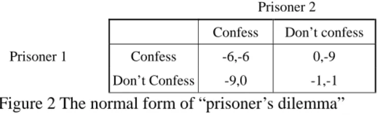
The normal form game expresses the players choosing their strategies independently and simultaneously. It is usually represented with a matrix. We depicted an example of normal form in Figure 2 by a well-known game called “the prisoner’s dilemma” below: Two players are ‘prisoner 1’ and ‘prisoner 2’; and ‘confess’ and ‘don’t confess’ are their strategies. The numbers in the cell are payoffs of two players.
Prisoner 2
Confess Don’t confess
Prisoner 1 Confess -6,-6 0,-9
Don’t Confess -9,0 -1,-1
Figure 2 The normal form of “prisoner’s dilemma”
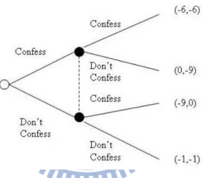
(1) Nodes: A position where a player makes a decision. (2) Branches: To represents the alternative choices or actions.
(3) Vectors: To represents the payoff of each player, listed in the order of players.
(4) Information sets: When two or more nodes are joined together by a dashed line. This means that the player whose decision it is dose not know which node he is at. When this situation occurs, the game is characterized as one of imperfect information. The extensive form of the same example is shown below:
Figure 3 The extensive form of “prisoner’s dilemma”
In extensive form games, more attention is placed on the sequence and on the amount of information available to each player when he is making a decision.
A solution to a game is a prediction of what each player in the game will do. There are many different solution techniques that have been proposed for different types of games. For static games, two kinds of solution techniques are widely applied. The first is using the concept of dominance. This technique is to obtain the solution by ruling out the strategies that a rational person would never play. The second is based on the concept of equilibrium. In a
non-cooperative game the equilibrium occurs when none of the player has an incentive to deviate from the predicted solution. The Nash equilibrium was introduced by John Nash, which pointed out that in equilibrium of each player’s strategy is optimal given that other player chooses the equilibrium strategy. If this is not the case, then at least one player would wish to choose a different strategy and so the situation would not be in the equilibrium any more.
Static games are what we can think of players making their decision simultaneously. However, sometimes the games are played over a number of time periods, it would become dynamic game. In a dynamic game, players are able to observe the actions of other players before making their optimal response. The extensive form can be a good way to describe a dynamic game. To solve the game, the backward induction is widely employed. Every finite game with perfect information can be solved by backward induction. It is the process of analyzing a game from back to front. At each information set, one strikes from consideration actions that are dominated, given the terminal nodes that can be reached (Watson, 2002).
A subgame is defined as a smaller part of the whole game starting from any one node and continuing to the end of the entire game, with the qualification that no information set is subdivided. In many dynamic games there are multiple Nash equilibria. These equilibria involve incredible threats or promises that are not in the interests of the players making them to carry out. The concept of subgame perfect Nash equilibrium rules out these situations. By requiring that a solution to a dynamic game must be a Nash equilibrium, it must comprise a Nash equilibrium in each of these subgame. That is to say, each player must act in his self-interest in every period of the game.
To sum up, the game theory is one of the theories for strategic decision. Under some basic assumptions, it applies the mathematical model to infer the behaviors between the players.
The most important assumption is that all the participants are rational. However, when a participant makes a decision, he would like to maximize his benefits by taking the opponent’s best policy into consideration. A lot of models have been developed to explain the behaviors of oligopolistic firms. In the next two subsections, we will introduce Cournot model and Stackelberg model that are related to our work.
2.1.1 Cournot Model
French economist Cournot developed the model in 1838. In this model, the players include two firms and produce homogeneous products. The available strategies are the quantities of product each firm can supply to the market. Here the both firms are assumed to be able to supply any positive level of output. The payoffs are the profits each firm receives. Both firms make their quantities decisions before knowing how many products the other firm has supplied to the market. Once each firm has chosen its optimal level of supply, the market price is also determined, and the firms can gain the corresponding level of profit.
To find the solution of this model, it begins with the reaction function. Each firm’s reaction function can be obtained by differentiating the firm’s profit function with respect to its own output level and then setting it to zero. Then rearranging the equation of this first-order condition, it leads to find a maximum solution. The second-order condition is checked to ensure that a maximum has indeed been found. In Nash equilibrium both firms must be maximizing profits simultaneously, given that their beliefs about the other firm’s level of supply.
The solution of this model is Pareto inefficient. It implies that there are other level of supply where at least one firm can be better off and the other firm no worse off. It also has some comments on Cournot model, such as it postulate that each firm can react to the other firm’s output level. This is inconsistent with the initial structure of the game where both firms set their
output level simultaneously. Besides, if the firms interact repeatedly, each firm assumes the other does not respond to the output changes would not be a rational conjecture.
2.1.2 Stackelberg Model
Stackelberg introduced this model in 1934. In this model, the players, the available strategies and the payoff setting are quite the same as in the setting of Cournot model. In Cournot model, both firms make their quantities decisions before knowing how many products the other firm has supplied to the market, that is, both firms choose their desired levels of supply simultaneously. Contrast to the Cournot model, the Stackelberg model assumed that at least one of the firms in the market is able to claim itself to a level of supply before the other firm in the market has decided its level of supply. The other firm observes the leader’s supply and then responds with its output decision. The firm that has the ability to claim its level of output initially is called the market leader, and the other firm is called the follower.
In the Stackelberg model, two firms involve to take actions in sequence. To solve this situation of the model, the backward induction approach will be employed. It starts with the last period first, initially determines the follower’s output decision. Given that the follower is rational, he will attempt to maximize his profit level, subject to the leader’s known level of supply. By differentiating the follower’s profit function with respect to the quantity and setting the equation to zero, it gives the first-order condition for a maximum. It shows the follower’s optimal response for any level of supply chosen by the leader, also known as the follower’s reaction function. By knowing the eventual outcome of the game in the last period, the leader will maximize his profits subject to this constraint. Replacing the output level of leader’s profit function with follower’s reaction function, it can obtain the first-order condition by differentiating the leader’s profit function with respect to it output level. This is subgame
perfect Nash equilibrium level of supply of the leader. Then applying this result into the follower’s reaction function, the follower’s best response can be acquired. The process can be summarized below:
(1) The follower’s reaction function is known by the leader.
(2) The leader applies the follower’s reaction function into his own profit function, in order to maximize his profit.
(3) The follower decides his own best action by applying the leader’s best policy.
With only one leader and one follower, the leader will produce the monopoly output level but not earn the monopoly profits because of the follower’s positive level of output. The Stackelberg equilibrium entails higher profits for the leader and smaller profits for the follower. It is said to be the first-move advantage.
2.2 Application of Game Theory in Supply Chain Models
Considerably amount of research have been done in the area of supply chain management from different point of view. Some researchers are interested in the inventory topic in supply chain. Arcelus and Srinivasan (1987) extend the deterministic EOQ model to reflect various optimizing criteria and alternative demand and price structure. They take inventories as investment rather than on traditional cost basis and use profits, return on investment and residual income to evaluate the inventory performance. Parlar and Wang (1994) focus on gaming nature of the discount problem and demand consideration to analyze the discounting decisions made by a supplier with a group of homogeneous customers. It shows that seller had to set up his quantity discount schedule such that the buyer would order more than his economic ordering quantity. By this, the seller could gain more from quantity discount. Fong et al. (2000)
considered an inventory model where two suppliers are used concurrently to replenish one stock item. The demand is assumed to be normally distributed and the supplier lead times are mixtures of Erlang distributions. The results present closed form expressions to evaluate the means and variance of the effective lead times, the probability of no stock out at a fixed reorder level and potential lost sales. When the lead times are not identical, it is possible to achieve a lower average stock level by using unequal order splits. Cachon (1999, 2001) studies the competitive and cooperative selection of inventory policies in a two-echelon supply chain with a supplier and N retailers. By using the theory of supermodular games, it shows that Nash equilibria exist in reorder point policies. But from a numerical result, the supply chain reorder point is frequently not a Nash equilibrium. Three cooperation strategies are presented to help improve supply chain performance: change incentives, change equilibrium, or change control. Among these, change control means that let vendor choose all reorder points. By this strategy, it would achieve optimal supply chain performance. Agrawal et al. (2002) consider that retailer faced the uncertain products demand and vendors’ difference in lead times, costs, and production flexibility. They develop an optimization model to choose the production commitments that maximize the retailer’s profit, given demand forecasts and vendors’ capacity and flexibility constrains. It helps the retailer to manage capacity, inventory and shipments of products produced by multiple vendors. Minner (2003) reviews inventory models with multiple supply options and discussed their contributions to supply chain management. The strategic aspects of supplier competition and the role of operational flexibility in global sourcing are emphasized. Some inventory problems from reverse logistics and multi-echelon supply chains are also mentioned.
Wong (2003) uses success factors of total quality management principles and concepts to develop supply chain management excellence model. Results support that the model would be useful for companies to achieve supply chain management excellence. Gunasekaran et al. (2004) think that the performance measurement pertaining to supply chain management has not received adequate attention from researchers and practitioners. They survey the literature and study the British companies to develop a framework of supply chain performance measurement. They conclude four major supply chain activities (plan, source, make/assemble, and deliver) and three planning level (strategic, tactical and operational) to be the core of framework. Yan (2008) use the Nash bargaining model to deal with the profit sharing in a manufacturer-retailer dual-channel supply chain. Chao et al. (2009) apply game theory to develop contractual agreements of products recall cost sharing between a manufacturer and a supplier to induce quality improvement.
To study supply chain in market economics view are also a great many. Kaihara (2001) proposes a supply chain management with market economics. His works takes the whole supply chain as a distributed resource allocation system, based on general equilibrium theory and competitive mechanism. By defining production functions and introducing budget constraint as an agent’s profit maximization strategy, supply chain management could lead to efficient resource allocations. Li and O’Brien (2001) use multiple-objective optimization model to match types of products to supply chain. Their results disclose some quantitative relationships between the performance of supply chain strategies and product attributes. These findings are also helpful to develop supply chain strategy by figuring out product assortments. Ertek and Griffin (2002) develop and analyze the case where supplier has dominant bargaining power and the case where buyer has dominant bargaining power. The buyer’s pricing scheme involves both a constant
markup and a multiplier. They conclude that buyer uses only a multiplier pricing scheme will lead to higher market price and the sensitivity when operational costs exist. The sensitivity of the market price increases nonlinearly as the wholesale price increased.
In the multi-echelon supply chain, some researchers argue the real world situation and then modify demand functions in supply chain models. They suggest that different demand functions would cause research results diversely. Lau and Lau (2003) argue that downward sloping demand curve is only valid for single echelon structure. When assuming different demand curve functions in a multi-echelon supply chain, it would lead to very different results. They have tried two-echelon and three-echelon situations. The results show that sometimes a very small change in demand curve would change the optimal solution drastically. Lau and Lau (2005) also argue that two-echelon symmetric-information and deterministic demand function are logically flawed. The results of one assuming demand curve cannot be safely generalized to other demand curve shapes. They propose a scenario with stochastic and asymmetric information to gain more plausible results. Leng and Parlar (2009) employ cooperative game to analyze cost saving allocation in a three-level supply chain by sharing demand information. The supply chain members cooperate with each other results in a cost reduction in the supply chain.
Choi (1991) analyze channel structure with two competing manufacturers and a powerful retailer under non-cooperative game. Some results depend critically on the form of demand functions. With a linear demand function, a manufacturer is better off by maintaining exclusive dealers while a retailer has an incentive to interact with several vendors. All channel members are better off when no one dominates the market. With a nonlinear demand function, an exclusive dealer channel provides higher profits to all members than a common retailer. The conclusion also emphasizes the importance of properly choosing the demand function. Parlar
and Wang (1994) take all-unit quantity discounting scheme into two-echelon system with a single vendor and a single retailer. They show that both parties could gain significantly from quantity discount policy under the manufacturer-Stackelberg structure. Weng (1995) further extends Parlar and Wang’s work to cover the two-echelon system with a single supplier and a group of homogeneous buyers. Both all-unit and incremental quantity discount policy are considered. The result presents that both discounting policies do the equal benefits to supplier and retailers. Li et al. (2002) work with supply chain in marketing view. They focus on cooperative advertising in marketing programs. A two-level supply chain is assumed and Stackelberg equilibrium is discussed. The results present different sharing rule in cooperative advertising expenditure. Leng and Parlar (2005) have reviewed the literatures in the supply chain management by using the game theory. They categorize the studies into five areas; however, most of them focus on the issues of inventory, production and pricing.
Yue et al. (2006) study the coordination of cooperative advertisement in a manufacturer-retailer supply chain when manufacturer offers price deductions to customers. Manufacturer acts as leader and the Stackelberg equilibrium is obtained for its decision on national advertisement, local advertisement, and manufacture’s share of local advertising allowance. The optimal price deduction is also determined. Xiao et al. (2010) are also focus on advertising investment and ordering quantity through the manufacturer-retailer contract. Yang and Zhou (2006) consider the pricing and quantity decisions of a two-echelon supply chain system with a manufacturer who produces a single product to two competitive retailers. The Stackelberg structure is assumed in that situation: The manufacturer acts as leader and duopolistic retailers act as followers. Their analyses focus on the competitive behaviors of duopolistic retailers and find that the degree of competitive situation would be influential to
pricing decision. The total profits of retailers would exceed the manufacture only under the situation that each retailer market demand is highly dissimilarity. He and Sethi (2008) study the dynamic optimal wholesale and retail prices and shelf-space allocation of a durable product supply chain consisting of a manufacturer and a retailer. By using Stackelberg model, the supply chain members’ strategies are discussed. Khouja and Zhou (2010) also use the Stackelberg game in the setting of a leader manufacturer and a follower retailer on mail-in rebate to discuss the issue of consumer surplus.
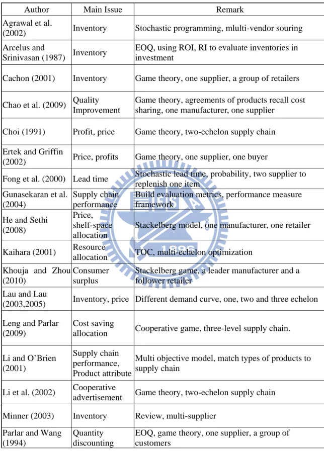
Most of the quantitative models related to supply chain management issues are dominated by the framework of multi-echelon systems or logistics/distribution systems. Besides, their backgrounds consider relationship between a single vendor and a single buyer or a single vendor and several buyers. The situation of multiple upstream manufacturers with downstream single retailer has received less attention. These main issues and the research methods of studies mentioned above are listed in Table 1. Here is one thing worthy of note. In previous subsection, the firms’ available strategies in original Cournot and Stackelberg models are level of output. But some later studies employ the Cournot or Stackelberg models which do not focus on the quantity competition. Most of them just borrow the idea of the players’ move pattern in the two models. Some works have taken the Cournot model as the players in the game reacting simultaneously and independently. As to Stackelberg model, some studies just borrow the concept of leader-follower interactive relationship of the players.
This study adopts a two-echelon supply chain, which comprises three members: two in upstream and one in downstream. In real world, it would stand for two manufacturers (vendors/suppliers) in upstream supply chain and a common retailer in downstream supply chain. By shifting the leader role of game theory in upstream and downstream firms, different scenarios
Table 1 Summary of the supply chain model literatures
Author Main Issue Remark
Agrawal et al.
(2002) Inventory Stochastic programming, mlulti-vendor souring
Arcelus and
Srinivasan (1987) Inventory
EOQ, using ROI, RI to evaluate inventories in investment
Cachon (2001) Inventory Game theory, one supplier, a group of retailers
Chao et al. (2009) Quality Improvement
Game theory, agreements of products recall cost sharing, one manufacturer, one supplier
Choi (1991) Profit, price Game theory, two-echelon supply chain Ertek and Griffin
(2002) Price, profits Game theory, one supplier, one buyer
Fong et al. (2000) Lead time Stochastic lead time, probability, two supplier to replenish one item
Gunasekaran et al. (2004)
Supply chain performance
Build evaluation metrics, performance measure framework He and Sethi (2008) Price, shelf-space allocation
Stackelberg model, one manufacturer, one retailer
Kaihara (2001) Resource
allocation TOC, multi-echelon optimization Khouja and Zhou
(2010)
Consumer surplus
Stackelberg game, a leader manufacturer and a follower retailer
Lau and Lau
(2003,2005) Inventory, price Different demand curve, one, two and three echelon Leng and Parlar
(2009)
Cost saving
allocation Cooperative game, three-level supply chain. Li and O’Brien
(2001)
Supply chain performance, Product attribute
Multi objective model, match types of products to supply chain
Li et al. (2002) Cooperative
advertisement Game theory, two-echelon supply chain Minner (2003) Inventory Review, multi-supplier
Parlar and Wang (1994)
Quantity discounting
EOQ, game theory, one supplier, a group of customers
continued Wong (2003) Supply chain
performance TQM principle, two case are studied Xiao et al. (2010)
advertising investment, ordering quantity
Game theory, one manufacturer, one retailer
Yan (2008) profit-sharing Nash bargaining model, one manufacturer, one retailer, dual-channel supply chain.
Yang and Zhou (2006)
Price, quantity,
profit Game theory, two-echelon supply chain Yue et al. (2006) Cooperative
Chapter 3 The Two-Echelon Supply Chain Models
As mentioned in the research background, the trend of powerful downstream member of a supply chain may be inevitable. In order to catch the point, the simplified two-echelon supply chain model is developed in our work comprising two members in upstream and one member in downstream, as depicted in Figure 4. The two upstream members are identified as the manufacturers and each of them produce one product. However, there is some extent of substitutability to the consumers between their products. The downstream member, who may be taken as the retailer, is responsible for selling the two products to the market.
Figure 4 The two-echelon supply chain model setting
There are four models derived from basic setting above. The first model assumes that upstream firms are independent and simultaneous reacting to the retailer, that is, each makes decision alone. The second model represents these two upstream members taking up collusion. Manufacturers/vendors have some extent coordination before their decisions to the downstream retailer. The third model applies the leader-follower interactive mechanism between the upstream members. The three models above are under the downstream firm-led situations,
where the retailer plays the leader role of the game structure in the two-echelon supply chain. The fourth model reverses the setting that upstream members act as the leader and the retailer acting as the follower. It provides the comparison to the previous three models with a traditional upstream dominating situation. All these models’ solution processes are applied with a backward induction approach in game theory. Some notations used in this study are briefly as follows:
i
q : the supply level of the product i.
i
p : the retail price of the product i.
i
w : the wholesale price of the product i.
i
a , b : demand function parameters of the product i. i
i
c : manufacturing cost of the product i.
θ: degree of substitutability between the products.
R
π , πM1, πM2: the profit of the retailer and manufacturers, respectively.
The solutions of the following models are conducted by backward induction, mainly to find the supply chain members’ decision under the game structure, including wholesale prices, retail prices and supply levels. Their profit can be obtained if the above solutions are determined. Due to the complexity of the analytical solutions, the demand function parameters, degree of substitutability and manufacturing cost will predefine in later numerical examples.
3.1 Model of Upstream Members Reacting Simultaneously and Independently
(R-S Model)
In this subsection we consider a two-echelon supply chain that consists of two upstream manufacturers and a common retailer. The products supplied by the two manufacturers exist to some extent substitutability to the customers. The interaction mechanism between the supply chain members is assumed to be the process in which the retailer acts as a leader and two manufacturers act as followers.
The demand function of the market is assumed to be a downward-sloping type: . 0 , 0 , 2 , 1 , , i i i j i i i i a b p p i j a b b q = − +θ = > > <θ < (1)
Here q denotes the deterministic market demand and i p the retail price in the market. The i
retailer first sets the product pricesp1, p2 to the duopolistic manufacturers, and then both
manufacturers simultaneously and independently respond with wholesale prices w ,1 w , 2
respectively. θ is as the degree of substitutability of the two products. Both manufacturers’ profit functions can be expressed as below:
), )( ( ) ( 1 1 1 1 1 1 1 1 2 1 w c q w c a b p p M θ π = − = − − + (2)
).
)(
(
)
(
2 2 2 2 2 2 2 2 1 2w
c
q
w
c
a
b
p
p
Mθ
π
=
−
=
−
−
+
(3) In (2) and (3), πMi represents each manufacturer’s profit, w the wholesale price per iunit charged to the retailer, and c the unit manufacturing cost. Thus, manufacturers 1 and 2 i
will maximize their profits with respect tow , 1 w . The optimal wholesale prices for the two are 2
, 1 2 1 1 1 1 1 1 b p p b c b a w = + − +θ (4) . 2 1 2 2 2 2 2 2 b p p b c b a w = + − +θ (5)
From the retailer’s point of view, since he realizes the manufacturers’ reaction functions, he will take them into consideration during the process in maximizing his profitπR. The profit comes from how many quantities of these two products sold and the retail prices set, so the profit function can be expressed below:
. ) ( ) (p1 w1 q1 p2 w2 q2 R = − + − π (6) Substituting (4) and (5) into (6) and solving ∂πR/∂p1=0 as well as ∂πR/∂p2=0 simultaneously, we obtain the retailer’s optimal sale prices *
1 p and * 2 p : , 2 2 2 1 1 2 2 3 2 1 2 * 1 R K b K R b a a p =θ + +θ + (7) * 1 2 1 1 1 2 2 3 1 2 , 2 2 a a b K b K p R R θ + θ + = + (8) whereK1 =a1 +b1c1, K2 =a2 +b2c2, 2 2 1 1 =4bb −θ R , R3 = bb1 2 −θ2. By applying (7) and
(8) into (4) and (5), each manufacturer’s wholesale price is:
, 2 2 2 1 2 1 2 1 * 1 R K K b c w = + +θ (9) . 2 2 2 1 1 2 1 2 * 2 R K K b c w = + +θ (10)
into (1): , 2 2 1 2 1 1 2 1 * 1 R R K b K a q = +θ − (11) * 2 1 2 2 2 2 1 2 2 a K b K R q R θ − = + , (12)
whereR2 =2b1b2 −θ2. As we get (6)-(12), it is now possible to find the profit functions of the
two manufacturersπM1, πM2; and the retailer’s profit functionπRbelow:
, 4 ) 2 )( ( 2 1 1 1 2 1 2 1 2 2 1 1 1 1 R R c K K b K R K b R a M − + − + = θ θ π (13) , 4 ) 2 )( ( 2 1 1 2 1 2 1 2 2 1 2 1 2 2 R R c K K b K R K b R a M − + − + = θ θ π (14) . 4 ) )( ( ) )( ( 3 1 3 2 1 1 2 2 2 1 2 1 2 3 1 2 2 1 1 2 2 1 1 1 R R R c a b a K R K b R a R c a b a K R K b R a R − + − + + − + − + = θ θ θ θ π (15)
3.2 Model of Upstream Members Acting in Collusion (C-S Model)
The second model introduced here is that both upstream manufacturers agree to act in union or after some extent of coordination in order to maximize their total profit. The upstream manufacturers can be recognized as one entity, and the two-level supply chain become the so-called successive monopolies in economics. The upstream total profit can be expressed as the sum of two manufacturers’ profit functions as below:
). )( ( ) )( ( 1 1 1 1 2 2 2 2 2 1 2 1 M w c a bp p w c a bp p M M π π θ θ π = + = − − + + − − + (16)
1 1 3 2 2 1 1 c p R a b a w = + θ + − , (17) 2 2 3 1 1 2 2 c p R a b a w = + θ + − . (18)
Since the retailer knows the wholesale price from each manufacturer, it will take all of their decisions into consideration and maximize its profit. By applying (17) and (18) into (6), and then solving ∂πR/∂p1=0and∂πR/∂p2 =0, the retailer’s optimal price would be:
3 2 2 1 1 * 1 4 ) ( 3 4 R a b a c p = + + θ , (19) 3 1 1 2 2 * 2 4 ) ( 3 4 R a b a c p = + + θ . (20)
Substituting (19) and (20) into demand function, the sale quantity can be determined:
) ( 4 1 2 1 1 1 * 1 a bc c θ q = − + , (21) ) ( 4 1 1 2 2 2 * 2 a b c cθ q = − + . (22)
The manufactures’ wholesale prices can also be obtained:
3 2 2 1 1 * 1 4 4 3 R a b a c w = + + θ , (23) 3 1 1 2 2 * 2 4 4 3 R a b a c w = + + θ . (24)
With original profit functions of each supply chain members, the profit would be determined as below:
) )( ( 16 1 2 1 1 1 3 1 2 2 1 1 θ θ π a bc c R c a b a M − + − + = (25) ) )( ( 16 1 1 2 2 2 3 2 1 1 2 2 θ θ π a bc c R c a b a M − + − + = (26) ) ) ( 2 2 2 ( 8 1 2 2 2 2 1 2 2 1 1 1 1 3 2 2 1 2 1 1 2 2 c b c c a c b c a R b a a a b a R − + − + + + + = θ θ π (27)
3.3 Model of Upstream Members in a Leader-Follower Structure (L-F Model)
In the third model we assume that one of the two firms (e.g., manufacturer 1) acts as a leader and the other (e.g., manufacturer 2) acts as a follower in upstream supply chain. For any given p , 1 p and2 w , the follower (manufacturer 2) observes its reaction function by 1
0 / 2 2 ∂ = ∂πM w and we get w2: 2 1 2 2 2 2 2b p m b K w = − +θ . (28)
Just as previous subsection, manufacturer 1 maximizes its profit, given the wholesale price of its rival. Replacing (28) into (2) and set∂πM1/∂w1 =0, we can getw as below: 1
2 2 1 2 1 1 2 2 1 2 ) 2 ( ) ( R m a b m c R K w =θ + − + +θ . (29)
Again, the retailer knows the manufacturers’ decisions and will maximize his own benefits. By applying (13) and (14) into the retailer’s profit function (6) and solving ∂πR /∂p1 =0 and∂πR/∂p2 =0, we get the retailer’s decision on market prices
* 1
p andp . The upstream *2
interactive mechanism makes the analytical solutions asymmetrical than previous two models. Due to the tedious of the closed-form solution, the results are listed in appendix. Some numerical results will be presented later.
3.4 Model of Upstream Members in Domination (M-D Model)
The fourth model is to represents the manufacturers as the leaders and the retailer as the follower. The profit functions of manufacturer 1, manufacturer 2, and the retailer are the same as (2), (3), and (6), respectively. The retailer’s reaction function is obtained by differentiating (6) with respect top and1 p . Set the equations to zero and solve simultaneously. We achieve: 2
) ( 2 1 3 2 2 1 1 1 R a b a w p = + + θ , (30) ) ( 2 1 3 1 1 2 2 2 R a b a w p = + + θ . (31)
By substituting (1), (30), and (31) into manufacturers’ profit functions (2) and (3), and then differentiating (2) and (3) and setting to zero, the manufacturers’ optimal wholesale prices are determined: 1 1 2 2 * 1 2 R K b K w =θ + , (32) 1 2 1 1 * 2 2 R K b K w =θ + . (33)
Putting (32) and (33) into (30) and (31), the retail prices are obtained:
) 3 2 ( 2 1 3 1 2 2 1 3 2 1 2 1 2 1 * 1 R R R b a R a R K c b b p = +θ + θ + , (34) ) 3 2 ( 2 1 3 1 2 1 2 3 1 1 1 2 2 1 * 2 R R R b a R a R K c b b p = +θ + θ + . (35)
Replacing the demand function with retailer prices (34) and (35), the supply level can also be obtained as below:
1 2 1 2 2 1 1 * 1 2 ) 2 ( R R c K b a b q = +θ − , (36) 1 2 2 1 1 2 2 * 2 2 ) 2 ( R R c K b a b q = +θ − . (37)
With the information above, the profits of supply chain members can be induced as follow: 2 1 2 2 1 2 2 1 1 1 2 ) 2 ( R R c K b a b M − + = θ π , (38) 2 1 2 2 2 1 1 2 2 2 2 ) 2 ( R R c K b a b M − + = θ π , (39) 3 2 1 3 1 2 2 2 1 2 1 2 1 1 2 2 1 1 2 2 3 2 1 1 1 2 2 2 1 1 2 2 1 2 2 1 1 4 ) ) ) 2 ( 2 ( 3 )( 2 ( ) ) ) 2 ( 2 ( 3 )( 2 ( R R R K K c b b R b a R a R c K b a b R K K c b b R b a R a R c K b a b R θ θ θ θ θ θ π = + − + + − − + + − + + − − . (40) This model is supposed to be the traditional upstream dominant situation in a supply chain, and is taken to contrast with the first three downstream firm-led models. The analytical solutions of these models (except L-F model) are presented in Table 2. In the next section, we are going to discuss some numerical examples to see how the dominant situation shifts influencing the decisions of supply chain members.
Table 2 Analytical solutions of the two-echelon supply chain models R-S C-S M-D * 1 p 1 1 2 2 3 2 1 2 2 2 2 R K b K R b a a + + +
θ
θ
3 2 2 1 1 4 ) ( 3 4 R a b a c +θ
+ (2 3 ) 2 1 3 1 2 2 1 3 2 1 2 1 2 1 R R R b a R a R K c b b + + +θ
θ
* 2 p 1 2 1 1 3 1 2 1 2 2 2 R K b K R b a a + + +θ
θ
3 1 1 2 2 4 ) ( 3 4 R a b a c +θ
+ (2 3 ) 2 1 3 1 2 1 2 3 1 1 1 2 2 1 R R R b a R a R K c b b + + +θ
θ
* 1 w 1 2 1 2 1 2 2 2 R K K b c +θ
+ 3 2 2 1 1 4 4 3 R a b a c +θ
+ 1 1 2 2 2 R K b K +θ
* 2 w 1 1 2 1 2 2 2 2 R K K b c +θ
+ 3 1 1 2 2 4 4 3 R a b a c +θ
+ 1 2 1 1 2 R K b K +θ
* 1 q 1 2 1 1 2 1 2 2 R R K b K a − +θ
( ) 4 1 2 1 1 1 bc cθ
a − + 1 2 1 2 2 1 1 2 ) 2 ( R R c K b a b +θ
− * 2 q 1 2 2 2 1 2 2 2 R R K b K a − +θ
( ) 4 1 1 2 2 2 bc cθ
a − + 1 2 2 1 1 2 2 2 ) 2 ( R R c K b a b +θ
− 1 Mπ
2 1 1 1 2 1 2 1 2 2 1 1 1 4 ) 2 )( ( R R c K K b K R K b R a +θ
− +θ
− ) )( ( 16 1 2 1 1 1 3 1 2 2 1θ
θ
c c b a R c a b a + − − + 2 1 2 2 1 2 2 1 1 2 ) 2 ( R R c K b a b +θ
− 2 Mπ
2 1 1 2 1 2 1 2 2 1 2 1 2 4 ) 2 )( ( R R c K K b K R K b R a +θ
− +θ
− ) )( ( 16 1 1 2 2 2 3 2 1 1 2θ
θ
c c b a R c a b a + − − + 2 1 2 2 2 1 1 2 2 2 ) 2 ( R R c K b a b +θ
− Rπ
(RS) 3 1 3 2 1 1 2 2 2 1 2 1 2 3 1 2 2 1 1 2 2 1 1 1 4 ) )( ( ) )( ( R R R c a b a K R K b R a R c a b a K R K b R a +θ − +θ − + +θ − +θ − Rπ
(CS) ( 2 2 2( ) ) 8 1 2 2 2 2 1 2 2 1 1 1 1 3 2 2 1 2 1 1 2 2 c b c c a c b c a R b a a a b a + + − + − + +θ
θ
Rπ
(MD) 1 1 2 2 1 2 2 1 1 2 2 2 1 1 1 2 3 2 2 2 1 1 2 2 1 1 2 1 2 1 2 2 2 1 3 4 ) ) ) 2 ( 2 ( 3 )( 2 ( ) ) ) 2 ( 2 ( 3 )( 2 ( R R R K K c b b R b a R a R c K b a b R K K c b b R b a R a R c K b a b +θ − θ + + − −θ + +θ − θ + + − −θChapter 4 Numerical Results
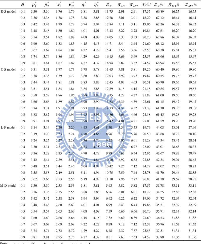
Due to the complexity of the analytical results, here we present some cases with different numerical setting to examine the results of supply chain members. The basic setting idea mainly comes from Yang and Zhou (2006), which article demonstrates the two-echelon supply chain model with one manufacturer dominating in upstream and two retailers in downstream. The variation of the degree of substitutability (θ) between two products are set from 0.1 to 0.9, which we can observe the change of optimal solutions and channel profit distribution. The profit is expressed by total upstream and downstream profit and how many percentages each member shares.
4.1 Two Identical Demand Functions
In the first case, the two upstream manufacturers are taken as identical. To the R-S model, two upstream members respond the downstream behavior individually, however, with the same manufacturing cost and demand function, their wholesale prices, supply volumes and profits are equal. The downstream retailer takes almost two-thirds of profit share.
If the upstream members act in union, like C-S model, the outcome shows that the collusion behaviors limit the supply levels and raise the wholesale prices. The retail prices are rise properly. The upstream members’ efforts have improved their profits, but not so much. Most of the profit share in the supply chain remains in the hand of downstream retailer. Although the retailer’s profits are less than that of R-S model, it still takes up more than the sum of the upstream members in our numerical example.
Under the L-F model, two upstream members compete with each other. The leader firm (manufacturer 1) provides lower price than the follower firm (manufacturer 2). Compared to
previous two models, both upstream members set the wholesale prices higher and sell more. Besides, the retail prices are lower than R-S and M-D models under the same degree of substitutability. Which implies the retailer loses its profit causes the upstream members more profits than before. The downstream retailer, although less profits here, still possesses the most part of profit shares.
The M-D model reveals the same retail prices, quantities and overall member profits as R-S model under the same degree of substitutability. As the substitutability increases, the wholesale price are going up, the manufacturers’ profit also rise. However, the upstream manufacturers own the domination of the supply chain. They charge the higher wholesale prices to the retailer and cause the profit distribution changes. Each supply chain member gets about one-third channel profits in our example. The entire outcomes are shown in Table 3.
Table 3 Numerical results that two upstream firms are identical θ * 1 p p2* w1* w*2 q1* q*2 πR πM1 πM2 Total πR% πM1% πM2% R-S model 0.1 3.30 3.30 1.76 1.76 3.81 3.81 11.75 2.91 2.91 17.57 66.89 16.55 16.55 0.2 3.36 3.36 1.78 1.78 3.88 3.88 12.28 3.01 3.01 18.29 67.12 16.44 16.44 0.3 3.42 3.42 1.79 1.79 3.94 3.94 12.84 3.11 3.11 19.06 67.36 16.32 16.32 0.4 3.48 3.48 1.80 1.80 4.01 4.01 13.43 3.22 3.22 19.86 67.61 16.20 16.20 0.5 3.54 3.54 1.82 1.82 4.08 4.08 14.05 3.33 3.33 20.70 67.86 16.07 16.07 0.6 3.60 3.60 1.83 1.83 4.15 4.15 14.71 3.44 3.44 21.60 68.12 15.94 15.94 0.7 3.67 3.67 1.84 1.84 4.22 4.22 15.41 3.56 3.56 22.53 68.38 15.81 15.81 0.8 3.74 3.74 1.86 1.86 4.29 4.29 16.15 3.69 3.69 23.53 68.66 15.67 15.67 0.9 3.81 3.81 1.87 1.87 4.37 4.37 16.94 3.82 3.82 24.57 68.94 15.53 15.53 C-S model 0.1 3.31 3.31 1.77 1.77 3.78 3.78 11.63 3.81 3.81 19.26 60.40 19.80 19.80 0.2 3.38 3.38 1.79 1.79 3.80 3.80 12.03 3.92 3.92 19.87 60.55 19.73 19.73 0.3 3.44 3.44 1.81 1.81 3.83 3.83 12.45 4.03 4.03 20.51 60.70 19.65 19.65 0.4 3.51 3.51 1.84 1.84 3.85 3.85 12.89 4.15 4.15 21.18 60.85 19.57 19.57 0.5 3.58 3.58 1.86 1.86 3.88 3.88 13.35 4.27 4.27 21.88 61.00 19.50 19.50 0.6 3.66 3.66 1.89 1.89 3.90 3.90 13.83 4.39 4.39 22.61 61.15 19.42 19.42 0.7 3.74 3.74 1.91 1.91 3.93 3.93 14.33 4.52 4.52 23.38 61.30 19.35 19.35 0.8 3.82 3.82 1.94 1.94 3.95 3.95 14.86 4.66 4.66 24.18 61.45 19.28 19.28 0.9 3.91 3.91 1.97 1.97 3.98 3.98 15.42 4.81 4.81 25.03 61.59 19.20 19.20 L-F model 0.1 3.14 3.14 2.20 2.20 4.63 4.61 8.70 5.54 5.53 19.76 44.03 28.01 27.96 0.2 3.19 3.20 2.23 2.24 4.70 4.66 8.96 5.79 5.76 20.50 43.68 28.22 28.10 0.3 3.24 3.25 2.27 2.28 4.76 4.70 9.22 6.05 6.01 21.28 43.34 28.42 28.24 0.4 3.30 3.31 2.31 2.32 4.83 4.75 9.50 6.32 6.27 22.09 43.01 28.63 28.37 0.5 3.36 3.38 2.35 2.36 4.90 4.79 9.79 6.62 6.54 22.95 42.67 28.83 28.49 0.6 3.42 3.44 2.39 2.41 4.97 4.84 10.10 6.92 6.82 23.85 42.34 29.04 28.62 0.7 3.48 3.51 2.44 2.46 5.04 4.89 10.42 7.25 7.12 24.79 42.02 29.25 28.73 0.8 3.55 3.58 2.49 2.51 5.11 4.94 10.75 7.59 7.44 25.78 41.70 29.46 28.85 0.9 3.62 3.65 2.53 2.56 5.19 4.99 11.10 7.96 7.77 26.83 41.38 29.67 28.95 M-D model 0.1 3.30 3.30 2.53 2.53 3.81 3.81 5.93 5.82 5.82 17.57 33.78 33.11 33.11 0.2 3.36 3.36 2.55 2.55 3.88 3.88 6.26 6.01 6.01 18.29 34.25 32.88 32.88 0.3 3.42 3.42 2.58 2.58 3.94 3.94 6.62 6.22 6.22 19.06 34.72 32.64 32.64 0.4 3.48 3.48 2.60 2.60 4.01 4.01 6.99 6.43 6.43 19.86 35.21 32.39 32.39 0.5 3.54 3.54 2.63 2.63 4.08 4.08 7.39 6.66 6.66 20.70 35.71 32.14 32.14 0.6 3.60 3.60 2.66 2.66 4.15 4.15 7.82 6.89 6.89 21.60 36.23 31.88 31.88 0.7 3.67 3.67 2.69 2.69 4.22 4.22 8.28 7.12 7.12 22.53 36.76 31.62 31.62 0.8 3.74 3.74 2.72 2.72 4.29 4.29 8.78 7.37 7.37 23.53 37.31 31.34 31.34 0.9 3.81 3.81 2.75 2.75 4.37 4.37 9.31 7.63 7.63 24.57 37.88 31.06 31.06 Note: a1 = a2 =20, b1 =b2 =5, c1 =c2 =1