國
立
交
通
大
學
電機與控制工程學系
博
士
論
文
以二維影像與漸進式相似度外觀圖解法
為基礎之穩健三維物體辨識
Robust 3D Object Recognition using 2D Views
via an Incremental Similarity-Based
Aspect-Graph Approach
研 究 生:蘇宗敏
指導教授:胡竹生 教授
以二維影像與漸進式相似度外觀圖解法為基礎
之穩健三維物體辨識
Robust 3D Object Recognition using 2D Views via an
Incremental Similarity-Based Aspect-Graph
Approach
研 究 生:蘇宗敏 Student:Tzung-Min Su
指導教授:胡竹生 Advisor:Jwu-Sheng Hu
國 立 交 通 大 學
電 機 與 控 制 工 程 學 系
博 士 論 文
A DissertationSubmitted to Department of Electrical and Control Engineering College of Electrical Engineering and Computer Science
National Chiao Tung University in partial Fulfillment of the Requirements
for the Degree of Doctor of Philosophy
in
Electrical and Control Engineering September 2006
Hsinchu, Taiwan, Republic of China
中華民國九十六年九月
以二維影像與漸進式相似度外觀圖解法
為基礎之穩健三維物體辨識
研究生:蘇宗敏
指導教授:胡竹生 博士
國立交通大學電機與控制工程學系(研究所)博士班
摘要
本論文提出了一套使用二維影像的穩健三維物體辨識架構。在此架構中包含 了兩個主要部份,第一部份是前處理的部份,用來抽取出二維影像中的前景物 體,以作為後續的學習與辨識之用。第二部份是一套漸進式資料庫建立方法,利 用從不同角度所拍攝到的三維物體之二維影像來建構出該三維物體資料庫,並且 能夠利用新拍攝到的二維影像來更新已建構好之三維物體資料庫。 在前處理的部份,我們提出了一套包含強光與陰影濾除的背景濾除架構 (BSHSR),使得前景物體在在光影變化與動態背景的影響下,依然能夠精確的被 萃取出來。BSHSR中包含了三個模型,分別是以色彩為基礎的機率背景模型 (CBM)、以CBM為基礎的梯度機率背景模型(GBM),以及一個圓錐形的光影模型 (CSIM)。CBM是利用高斯混合模型(GMM)針對每個像素的像素值作統計所建構 出來的模型。而根據CBM,又可以建構出短期背景模型(STCBM)與長期背景模 型(LTCBM),接著再利用STCBM與LTCBM建構出GBM。而為了區別前景、強 光與陰影的不同,本研究中提出了一建構在RGB色彩空間中且具有動態錐形邊界 的CSIM。在漸進式資料庫建立方法的部份,我們提出了一套以相似度外觀圖解 法為基礎的學習架構(ISAG)。利用相似度外觀圖解法,每個三維物體在資料庫中 均可用一組外觀(aspect)來表示,而每一個外觀則包含了數目不一的二維影像, 並且用一個特徵面(characteristic view)來代表。本研究所提出的漸進式資料庫建 立方法,目的在於提高屬於同一外觀的二維影像彼此之間的相似度,並且降低各 個特徵面彼此之間的相似度。此外,為了模擬人類認知物體的能力,我們採用隨 機取樣之角度所拍攝的三維物體之二維影像來做為訓練影像,隨著所收集到的二 維影像數目增加,該三維物體的資料庫也會隨之更新。最終,本論文先以實際複 雜環境中所拍攝的數段影片之實驗結果來說明所提出的BSHSR之可行性,接著 將BSHSR應用於三維物體辨識架構中,以抽取出二維影像中之前景物體。而為 了驗證所提出三維物體辨識架構之優越性,我們利用ISAG搭配物體的形狀與色 彩特徵,將之應用於三種不同的三維物體之問題,分別是剛體辨識、人形姿態辨 識與場景辨識,並根據辨識率結果來說明所提出的三維物體辨識架構之可行性。Robust 3D Object Recognition using 2D Views
via an Incremental Similarity-Based
Aspect-Graph Approach
Graduate Student: Tzung-Min Su Advisor: Dr. Jwu-Sheng Hu
Department of Electrical and Control Engineering
National Chiao-Tung University
Abstract
This work presents a framework for robust recognizing 3D objects from 2D views. The proposed framework comprises of two stages: the pre-processing stage and the incremental database construction stage. In the pre-processing stage, foreground objects is extracted from 2D views and applied for building 3D database and recognizing. In the incremental database construction stage, a 3D object database is built and updated using 2D views randomly sampled from a viewing sphere.
A background subtraction scheme involving highlight and shadow removal (BSHSR) is proposed as the pre-processing stage of the framework. Foreground regions can be precisely extracted from 2D views using the BSHSR despite illumination variations and dynamic background. The BSHSR comprises three models, called the color-based probabilistic background model (CBM), the gradient-based version of the color-based probabilistic background model (GBM) and a cone-shape illumination model (CSIM). The Gaussian mixture model (GMM) is applied to construct the CBM using pixel statistics. Based on the CBM, the short-term color-based background model (STCBM) and the long-term color-based background model (LTCBM) can be extracted and applied to build the GBM. Furthermore, a new
dynamic cone-shape boundary in the RGB color space, called the CSIM, is proposed to distinguish pixels among shadow, highlight and foreground.
An incremental database construction method based on similarity-based aspect-graph (ISAG) is proposed for building the 3D object database using 2D views. Similarity-based aspect-graph, which contains a set of aspects and characteristic views for these aspects, is employed to represent the database of 3D objects. An incremental database construction method that maximizes the similarity of views in the same aspect and minimizes the similarity of prototypes is proposed as the core of the framework. To imitate the ability of human cognition, 2D views randomly sampled from a viewing sphere are applied for building and updating a 3D object database. The effectiveness of the BSHSR is demonstrated via experiments with several video clips collected in a complex indoor environment. The BSHSR is applied in the proposed framework to extract foreground object from 2D views. The proposed framework is evaluated on various 3D object recognition problems, including 3D rigid recognition, human posture recognition, and scene recognition. Shape and color features are employed in different applications with the proposed framework to show the efficiency of the proposed method.
致 謝
對於本論文的完成,首先要感謝的是我的指導教授 胡竹生教授,感謝老師 在我的碩士班與博士班這七年來,給予我相當多珍貴的意見與指導,往往能夠讓 我茅塞頓開,並且能從許多層面去思考問題。這段時間也從老師身上學到了許多 研究的態度與寶貴的知識,讓我能夠用更成熟與積極的態度來面對自己的研究。 而除了課業之外,老師也給予我關於感情、婚姻與生涯規劃方面的建議,並且在 我遇到低潮的時刻給予我鼓勵,真的很感謝老師。此外,也很謝謝老師給予我機 會去參與許多比賽與研究計畫,讓我能夠有機會獲得更多的磨鍊,也因而有機會 在 2002 年 9 月份跟老師ㄧ起到英國參加 CCA 2002 研討會,並且參觀了牛津大學、 劍橋大學、IEE 學會、大英博物館、白金漢宮、Glasgow 與愛丁堡等等地點,都 是讓我很難忘的回憶。在此,誠摯的致上我最真摯的謝意,謝謝老師。 另外,首先要感謝一起執行數位化居家照護系統三年計畫的學弟妹們,感謝 幽默又搞笑的士奇,你是我認識的朋友裡面,唯一一位可以跟打掃工五館的特殊 小孩們玩在一起的人,可見你一定很有愛心以及具備特殊的吸引力。感謝住在信 義區的小開群棋,你敦厚老實的個性搭配害羞的笑容,總有一天可以找到你的真 命天女。感謝認真又細心的佩靜,妳專情與顧家的個性,真的是很值得讚許。感 謝搞笑又無厘頭的恆嘉,沒想到你是減肥界的達人,我是從你口中才知道珍珠奶 茶的熱量有多驚人。感謝為愛走天涯的弘齡,相信你因為美國之行而成長了許多。 接著要感謝 88 級的學長們,感謝傳承實驗室管理員給我的 DSP 達人鴻志學 長,以及幽默的凱學長,感謝你們兩位耐心的教導我 DSP 相關知識,感謝親切的 瓊宏學長,謝謝你常常跟我分享影像相關知識以及鼓勵我。感謝 RTOS 達人小陶 子學長,實作實力超強的你,讓我非常的敬佩,另外,想不到你對於駭客破解技 術頗有研究。感謝話不多但是實力很強的邦正學長,以及感謝溫文儒雅的俊德學 長,每次跟你聊天,心情都相當棒。 感謝 89 級同屆進入實驗室的學長與同學,感謝執行力超強的立偉學長,你對機器人總有說不完的理想,時間對於你來說也總是不夠用,從你身上我學到了 許多做事情應有的態度,也很懷念那時候跟你參加 ICM/HIMA 2005 研討會的時 候,一起到士林夜市逛街聊天。再來要感謝跟我認識 14 年,高中同校、大學同 系、研究所與博士班都同一位指導教授、博士班論文口試同一天,甚至連國防役 服役公司都是頗有淵源的兩家公司的維瀚,真的是很有緣分啊! 革命情感也不用 多說了!一起修課、參加比賽、寫 DSP 程式、寫論文,真的很多很多的回憶啊! 接 著要感謝桌球很強、又很會吃炸冰淇淋的价呈,記得當年到台南比賽以及到嘉義 參加 AMTE 2002 研討會的時候,一起住在飯店準備比賽資料與投影片,在校時間 一起修課、逕讀博士班、打羽球、玩三國志、CS…,留下許多許多美好的回憶~ 而 講到 CS,就讓我想到欣慈,每次玩 CS 的時候,妳的反應總是讓大家記憶深刻啊 ~ 此外,也相當懷念當年跟妳一起在影像領域研究的日子,跟妳討論之後,總是 能有許多不同的體驗。最後,感謝已經改名為峻葦的家銘,你既是我大學同班同 學也是我系學會的夥伴,在研究所的那兩年中,除了見識到你小畫家的功力之 外,也感染到你在研究上的熱情。 感謝後來常常跑去 DSP 實驗室的德琪,妳最後的論文成果果然是相當豐碩啊 ~感謝每次來參加聚會都讓人感覺越來越瘦的嘉芳,也感謝上次到妳公司面試 時,妳在公司陪我聊了那麼久。感謝超有想法的阿鎧,很懷念那時候跟你一起跑 環校,可惜你到最後切了西瓜,然後一直被記到現在,為了怕知道這件事情的學 弟都畢業了,請原諒我繼去年价呈提了一次之後,今年又再度提了一次。感謝已 經改名為昊群的青衛,記得當年跟你與价呈一起討論財經話題,雖然討論的結果 跟未來的發展都不盡符合,但還是相當有趣的一段回憶。感謝很像王力宏的 Alan(葉威廷),帥氣的你事業愛情兩得意,每每都能從你那邊得到許多業界的訊 息。感謝重視養生的倉億,我從你那邊學到了許多中藥的知識,還得到了一張你 說經過氣功師父加持過的卡片。 感謝思考獨特但總是讓人誤會有在吸毒的春成,感謝作風海派但心思細膩的 Angel(蔡銘謙),感謝專情又積極上進的家瑋,感謝認真負責的億如,感謝喜歡
說冷笑話然後也很好笑的順智,感謝會煮紅豆湯、會做小卡片的康康,感謝吃素 的俊德跟我分享交友經驗談,感謝很 man 的佳興,跟你一起到上海參加 CASE 2006 的那一個禮拜,讓我留下許多美好的回憶,此外,每次吃飯時間跟你討論財經與 感情話題,也讓我有許多收穫,感謝減肥界達人鏗元,每次打開實驗室冰箱,總 是可以感受到妳的存在,感謝被稱為實驗室一姊的岑思,想不到妳那麼在意被別 人踩到鞋子,也希望下次能看到妳攜伴參加聚會喔!感謝很有衝勁的晏榮,感謝 具有貴賓狗命的藍蕙,妳總是帶給我們最棒的運氣,感謝也很 man 的耀賢,還記 得那天大家一起玩牌的時候,你的演技真的是頗不賴喔!感謝很憨厚又很疼女友 的榮煌,感謝信主而不能說謊的永融,你認真的研究態度感染的身邊的所有人, 感謝常常熬夜爆肝但肝指數都很正常的 Alphar,感謝具備多種才藝的凱祥,另 外,也要感謝還在實驗室的學弟妹們:感謝上次幫我搬家的俊宇、感情快要開學 的啟揚、很有研究熱忱的阿吉、很耐操的可以做實驗 12 個小時以上的 PaPa、聽 說唱歌很好聽的治宏、愛喝葡萄柚青茶的瓊文、畢業生代表鎮宇、白白淨淨的明 堂、有正妹同學的源松以及常常打扮很時髦的育綸。 另外,也要感謝我的室友益生,從你那邊我學到了許多關於論文投稿的知 識,跟你一起討論佛教話題也讓我獲益匪淺,感謝常常借我車的室友仁乾,你對 於法輪功的熱忱,讓我非常的敬佩! 感謝還沒畢業就已經在外面工作很久的室友 盟淳,感謝你提供我許多在業界的經驗談,讓我找國防役的時候能夠更有信心, 也要感謝我早期的室友豐洲跟與豐洲的女友文真,感謝你們在我低潮的時候給我 鼓勵與支持,也要感謝我的高中同學們,每年一次的同學會都讓我充滿了期待。 最後,衷心的感謝我的家人,感謝我的爸爸與媽媽,讓我在唸書的這段時間,一 直都沒有後顧之憂,可以專心唸書,並且持續的給予我關心與溫暖。感謝我的兩 位妹妹,每當我回家,都會給予我最溫暖的關懷。也要感謝認識了 17 年,交往 了 9 年的女友雅婷,感謝妳一直扮演我生命中的重要角色,妳持續的關心與鼓 勵,一直是我在求學路上重要的力量。謝謝在我生命中的這些貴人,因為有您們 的關心,讓我能夠用正面積極的態度來面對人生的旅途,有您們真好!
Contents
Chapter 1 Introduction ...1
1.1 Overview of 3D Object Recognition ...1
1.1.1 3D Object Recognition ...1
1.1.2 Human Posture Recognition ...2
1.1.3 Scene Recognition ...3
1.2 Overview of Background Subtraction ...4
1.3 Outline of Proposed System...6
1.3.1 Background Subtraction...6
1.3.2 3D Object Recognition ...7
1.4 Contribution of this Dissertation...8
1.5 Dissertation Organization ...9
Chapter 2 Background Subtraction...10
2.1 Introduction...10
2.2 System Architecture...11
2.3 Background Modeling ...12
2.3.1 Color-Based Background Modeling ...12
2.3.2 Model Maintenance of the LTCBM and STCBM ...15
2.3.3 Gradient-Based Background Modeling ...20
2.4 Background Subtraction with Shadow Removal ...23
2.4.1 Shadow and Highlight Removal ...23
2.4.2 Background Subtraction...27
Chapter 3 Incremental Similarity-Based Aspect-Graph 3D Object Recognition .29 3.1 Introduction...29 3.2 System Architecture...32 3.3 Object Representation...34 3.3.1 Shape Features ...34 3.3.2 Color Features...36 3.3.3 Similarity Functions...38 3.3.4 Similarity Measures ...38
3.4 Flexible 3D Object Recognition Framework...39
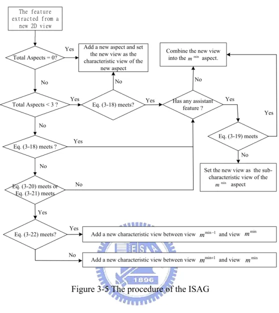
3.4.1 Generation of Aspects and Characteristic Views ...40
3.4.2 Object Recognition using 2D Characteristic Views...43
3.4.3 Applications ...44
Chapter 4 Experimental Results...47
4.1.1 Local Illumination Changes...48
4.1.2 Global Illumination Changes ...53
4.1.3 Foreground Detection ...55
4.1.4 Dynamic Background ...55
4.1.5 Short-Term Color-based Background Model (STCBM) ...58
4.2 3D Object Recognition ...59
4.2.1 Rigid Object Recognition ...63
4.2.2 Human Posture Recognition ...67
4.2.3 Scene Recognition ...69
Chapter 5 Conclusions and Future Researches...74
5.1 Conclusions...74
5.2 Future Researches ...77
Index
Assistant 3D object databases (AOD)...32
Background subtraction scheme involving highlight and shadow removal (BSHSR) .iv Candidate color-based background model (CCBM)...16
Color-based probabilistic background model (CBM)...iv
Cone-shape illumination model (CSIM)...iv
Elected color-based background model (ECBM) ...15
Expectation maximization (EM)...13
Fourier descriptor (FD) ...34
Gaussian mixture model (GMM)...iv
Gradient-based version of the color-based background model (GBM)...iv
Gradient Vector Flow Snake (GVF) ...34
Incremental database construction method based on similarity-based aspect-graph (ISAG)...v
Long-term color-based background model (LTCBM) ...iv
Main 3D object database (MOD)...33
Maximum likelihood (ML) ...13
Multicolored Region Descriptor (M-CORN)...1
Point-to-point length (PPL)...34
Principal component analysis (PCA) ...3
List of Figures
Figure 1-1 Block diagram of proposed 3D object recognition system. ...6
Figure 1-2 Block diagram of foreground detection. ...7
Figure 1-3 Block diagram of 3D object recognition...7
Figure 2-1 The block diagram of the BSHSR...11
Figure 2-2 Block diagram showing the process of building the initial LTCBM, ECBM and CCBM. ...16
Figure 2-3 Block diagram showing the process to calculate H . ...20 CG Figure 2-4 The proposed 3D cone model in the RGB color space. ...24
Figure 2-5 2D projection of the 3D cone model from RGB space onto the RG space. ...25
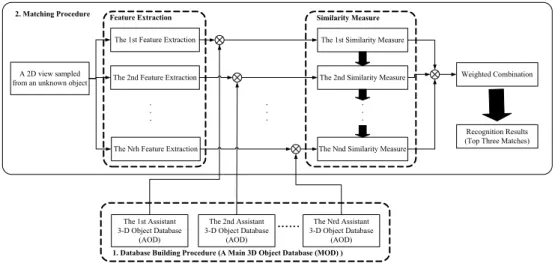
Figure 3-1 The system architecture of the proposed framework. A MOD comprises of total AODs. ...33
Figure 3-2 The database building procedure, where T is the number of objects in 0 the database and T is the number of sampled views required to build the 1 aspect-graph representation of an object...33
Figure 3-3 The inner structure of an AOD...33
Figure 3-4 5D feature vector construction...36
Figure 3-5 The procedure of the ISAG...42
Figure 4-1 The results of illumination changes with a yellow desk light, the number below the picture is the index of frame...50
Figure 4-2 The results of illumination changes with white desk light, the number below the picture is the index of frame...52
Figure 4-3 The results of global illumination changes with fluorescent lamps, the number below the picture is the index of frame. ...54
Figure 4-4 The results of foreground detection. ...56
Figure 4-5 The results of background subtraction about dynamic background...57
Figure 4-6 The results of the advantage of the STCBM, where the red color means the shadow, the green color means the highlight and the blue color means the foreground. ...59
Figure 4-7 The first database containing 12 3D rigid objects...60
Figure 4-8 The second image database containing eight 3D human postures...60
Figure 4-10 The system architecture of the proposed framework applied on the first experiment (3D rigid object recognition). ...64 Figure 4-11 Recognition rates of coarse and fine databases (D18,D36,D54,D72,D90 and
108
D ), calculated using 200 results...66
Figure 4-12 Standard deviations of recognition rates using coarse to fine databases (D18,D36,D54,D72,D90 and D108), calculated using 200 results...67 Figure 4-13 The system architecture of the proposed framework applied on the second experiment (human posture recognition). ...68 Figure 4-14 The indoor environment from which scenes in the third database are obtained...70 Figure 4-15 The sample training image, blob model and conceptual description of each scene captured in the indoor environment (Fig. 4-14)...70 Figure 4-16 The system architecture of the proposed framework applied on the second experiment (human posture recognition). ...71 Figure 4-17 The 11 characteristic views at the 6th position in the indoor environment. ...71 Figure 4-18 The test images captured from the 6th position in the indoor environment. ...71 Figure 5-1 The aspect-graph representation of the first human posture listed in Fig. 4-8 via MAG only. ...76 Figure 5-2 3D object recognition system with a combination of a feature predictor and the proposed method illustrated in Fig. 1-3. ...77 Figure 5-3 3D object recognition system with an efficient searching algorithm...78
List of Tables
Table 2-1 An example to calculate CG histogram ...19 Table 4-1 The robustness test between the proposed method and that proposed by Hoprasert [60] via local illumination changes with a yellow desk light...49 Table 4-2 The robustness test between the proposed method and that proposed by Hoprasert [60] via local illumination changes with a white desk light...51 Table 4-3 The comparison between the proposed method and that proposed by Hoprasert [60] via global illumination changes with fluorescent lamps ...53 Table 4-4 The comparison between the proposed method and that proposed by Hoprasert [60] via foreground detection...55 Table 4-5The threshold values for the ISAG ...62 Table 4-6 The result of rigid object recognition using 2D views via MAG and PPL..64
Table 4-7Results for numbers of aspects using MAG and PPL after updating with
additional training views...65
Table 4-8Results of human posture recognition using 2D views via MAG and θz ..68
Table 4-9 Human posture recognition results using 2-D views via BM with position variations and different level of occlusion...73
Chapter 1
Introduction
1.1 Overview of 3D Object Recognition
1.1.1 3D Object Recognition
Object recognition is an important topic in computer vision where various approaches have been developed [1-5]. However, numerous technical issues require further investigation, especially for 3D object recognition. Variations in viewing direction and angle [1, 6-7], illumination changes [8-9], and scene clutter and occlusion [10-11] are the main challenges for object recognition. In recent years, many researches were presented for solving these issues. For example, a generic object class detection system [12] that combines the Implicit Shape Model and multi-view specific object recognition is presented to detect object instances from arbitrary viewpoints. A new framework [13] that combines a visual-cortex-like hierarchical structure and an increasingly complex and invariant feature was proposed for robust object recognition. Furthermore, a new object representation, Multicolored
Region Descriptor (M-CORN) [14], was proposed to describe the color and local
shape information of objects. Moreover, some low-level visual features, such as
object shading, surface texture and an object’s contour or binocular disparity, have recently been proposed to describe 3D object representation [15-19]. However, 3D object recognition is primarily influenced by position variations and illumination source type, and the relative positions of an observer and object.
Some advanced theorems of 3D object perception have been investigated to solve these issues and enhance the 3D object recognition task [20]. Existing theorems for high-level 3D object perception can be categorized as object-centered and viewer-centered representations based on a coordinate system [2], and as volume-based (or model-based) and view-based representations based on the constituent elements [21]. Viewer-centered representation describes portions of an object relative to a coordinate system based on an observer. A view-based representation characterizes a 3D object using a set of object views. Both viewer-centered and view-based frameworks conform to the intuition of human perception, during which a person memorizes an object using several primary views without requiring an exhaustive 3D object model. Moreover, S. Kim et al. [22] proposed a combined model-based method to recognize 3D objects using a combination of a bottom-up process (model parameter initialization) and a top-down process (model parameter optimization).
1.1.2 Human Posture Recognition
Human posture recognition is an important example of 3D object recognition. A considerable number of studies have been made on this field over the past 10 years [23-24]. Existing approaches [25] for human posture recognition are classified as
direct and indirect approaches based on the human body model. The model has either a 2D or 3D representation based on the dimensionality of features. The direct approach typically consists of a detailed human body model. For example, Ghost [26] developed a silhouette-based body model, incorporating hierarchical body pose estimation, a convex hull analysis of the silhouette and a partial mapping from body parts to silhouette segments. Furthermore, Pfinder [27] utilized color information to develop a multi-class statistical model and identified human body parts using shape detection. However, occlusions and perspective distortion lead to the unreliable results. The indirect approach extracts features about the human body instead of a detailed human body model, and combines classifiers to estimate human posture. For example, Ozer et al. [28] utilized the AC-coefficients as the features and adopted principal component analysis (PCA) as the classifier. A recent work [29] used color, edge and shape as the features and the hidden Markov model as the classifier. Furthermore, complex 3D models utilize different equipment to solve problems associated with the angle from which human postures are observed. For instance, Delamarre et al. [30] proposed a method for building a 3D human body via three or more cameras, and then calculated the projection of the silhouette for comparison with 2D projections in a database. Additionally, 3D laser scanners [31] or thermal cameras [32] have also been adopted to build a 3D human body model. However, these 3-D solutions require enormous computing time and high device costs.
1.1.3 Scene Recognition
Recognizing scene can be addressed as a problem of 3D object recognition, where the scene represents variations due to changing the viewer location or camera pose [33-39]. Scene recognition is a fundamental element in the topological representation
of environment [40-41], where the graph node of the adjacency graph describes the robot’s location. Moreover, scene recognition can also be employed to memorize and detect visual landmarks in geometrical representation of environments [42-43]. In [44], a series of experiments were presented to show that only the overall geometry and a few key features are required to perform scene recognition. For capturing the key features, Kröse et al. [45] proposed a method for appearance-based modeling of an environment by extracting scene features using PCA. Oliva et al. [46] proposed a scene-center-based approach to estimate the structure of a scene image by the mean of global image features. Moreover, a framework combined with a supervised method for recognizing the door and an unsupervised method for learning door-reaching behavior has been proposed in [47].
1.2 Overview of Background Subtraction
A reference image is generally used to perform background subtraction. The simplest means of obtaining a reference image is by averaging a period of frames [48]. However, it is not suitable to apply time averaging on the home-care applications because the foreground objects (especially for the elderly people or children) usually move slowly and the household scene changes constantly due to light variations from day to night, switches of fluorescent lamps and furniture movements etc. In short, the deterministic methods such as the time averaging have been found to have limited success in practice. For indoor environments, a good background model must also handle the effects of illumination variation, and the variation from background and shadow detection. Furthermore, if the background model cannot handle the fast or slow variations from sunlight or fluorescent lamps, the entire image will be regarded as foreground. That is, a single model cannot represent the distribution of pixels with
twinkling values. Therefore, to describe a background pixel by a bi-model instead of a single model is necessary in home-care applications in the real world.
Two approaches were generally adopted to build up a bi-model of background pixel. The first approach is termed the parametric method, and uses single Gaussian distribution [27] or mixtures of Gaussian [49] to model the background image. Attempts were made to improve the GMM methods to effectively design the background model, for example, using an on-line updated algorithm of GMM [50] and the Kalman filter to track the variation of illumination in the background pixel [51]. Furthermore, motion information is used for extracting a set of regions that have coherent motion to improve the efficiency of region classification and computing time [52]. The second approach is called the non-parametric method, and uses the kernel function to estimate the density function of background images [53].
Another important consideration is the shadows and highlights. Numerous recent studies have attempted to detect the shadows and highlights. Stockham [54] proposed that a pixel contains both an intensity value and a reflection factor. If a pixel is termed the shadow, then a decadent factor is implied on that pixel. To remove the shadow, the decadent factor should be estimated to calculate the real pixel value. Rosin [55] proposed that shadow is equivalent to a semi-transparent region, and uses two properties for shadow detection. Moreover, Elgammal et al. [53] tried to convert the RGB color space to the rgb color space (chromaticity coordinate). Because illumination change is insensitive in the chromaticity coordinate, shadows are not considered the foreground. However, lightness information is lost in the rgb color space. To overcome this problem, a measure of lightness is used at each pixel [53]. However, the static thresholds are unsuitable for dynamic environment.
1.3 Outline of Proposed System
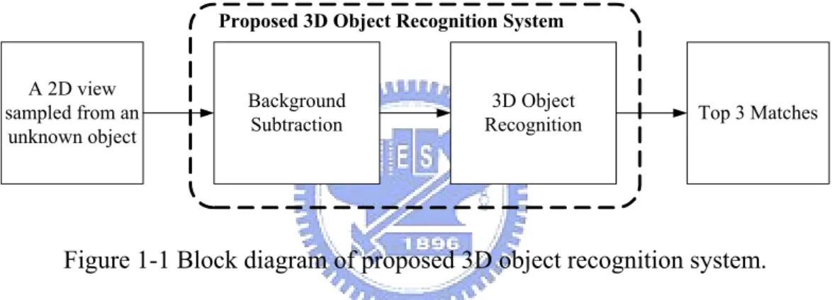
Figure 1-1 illustrates the block diagram of the proposed framework. In the foreground detection block, image pixels of a 2D view are classified among foreground, shadow, highlight and background. The foreground pixels are applied to extract features for 3D object recognition. In the 3D object recognition block, one or more similarity measures are applied on the extracted features of a testing 2D view and all the objects in a 3D object database. The top three similar objects in the database (Top 3 Matches) are regarded as the recognition results.
A 2D view sampled from an unknown object Background Subtraction 3D Object
Recognition Top 3 Matches
Proposed 3D Object Recognition System
Figure 1-1 Block diagram of proposed 3D object recognition system.
1.3.1 Background Subtraction
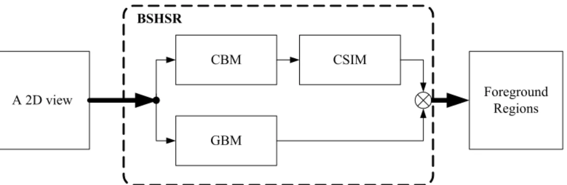
In the background subtraction block (Fig. 1-2), a background subtraction scheme with highlight and shadow removal (BSHSR) is proposed to extract foreground regions with three proposed background models. First, the CBM is applied for extracting foreground candidates pixels. After that, the CSIM is applied for classifying foreground candidate pixels among real foreground, shadow and highlight. Finally, the GBM is used for eliminating false foreground pixels from the foreground candidate pixels. Moreover, only those real foreground pixels are reserved for further processing.
CBM
GBM
CSIM
A 2D view Foreground Regions
BSHSR
Figure 1-2 Block diagram of foreground detection.
1.3.2 3D Object Recognition
In the 3D object recognition block (Fig.1-3), a main 3D object database (MOD) is built during the building procedure with the proposed incremental similarity-based aspect-graph (ISAG). After that, one or more features are extracted from those foreground region to measure similarity among the objects in the MOD. After a weighted combination of all similarity measures, the top 3 similar objects are regarded as the recognition results.
Feature Extraction Foreground
Regions Top 3 Matches
3D Object Recognition Similarity Measure Matching Procedure Weighted Combination Incremental Similarity-Based Aspect-Graph (ISAG) A Main 3D Object Database (MOD) Building Procedure
1.4 Contribution of this Dissertation
The problem we address in this work is as follows: Given a set of 2D views of 3D objects, such as rigid objects, human postures, and scenes, how do we represent these 3D objects with collected 2D views in an efficient way? In other words, how do we extract the representative views from these 2D views such that a 3D object can be indexed efficiently? For the purpose of this work, we propose a flexible 3D object recognition framework for building the 3D object database and recognizing 3D objects with 2D views. We place emphasis on three issues in practice, which are listed as follows.
1. For extracting the object features from a complex background, a background
subtraction scheme involving highlight and shadow removal (BSHSR) is proposed as the pre-processing stage of the framework. Foreground regions can be precisely extracted from 2D views using the BSHSR despite illumination variations and dynamic background. The BSHSR comprises three models, called the color-based probabilistic background model (CBM), the gradient-based version of the color-based probabilistic background model (GBM) and a cone-shape illumination model (CSIM).
2. An incremental database construction learning method based on similarity-based
aspect-graph (ISAG) is proposed for building the 3D object database using 2D views. The accuracy of the object representation increases with minimal growth of search space while collecting additional new object views.
3. For improving the robustness and computing time, a hierarchical matching
structure is proposed to decide the final recognition result with a weighted combination of the results from multiple features.
1.5 Dissertation Organization
This chapter provides a brief introduction of the background subtraction system and 3D object recognition, including rigid object recognition, human posture recognition and scene recognition. This chapter also briefly discusses two main components in the proposed 3D object recognition framework. The remainder of this dissertation is organized as follows. Chapter 2 presents the proposed background subtraction algorithm (BSHSR), including the descriptions of the CBM, STCBM, LTCBM, GBM, and CSIM. Chapter 3 describes the ISAG and the proposed hierarchal matching structure. Chapter 4 presents experimental results that demonstrate the performance of the proposed method for 3D rigid objects, human postures and scene recognition. Finally, some concluding remarks and future researches are discussed in Chapter 5.
Chapter 2
Background Subtraction
2.1 Introduction
For precisely extracting foreground objects, environmental changes and shadow/highlight effects are necessary to be considered. Despite the existence of abundance of research on individual techniques, as described in Chapter 1, few efforts have been made to investigate the integration of environmental changes and shadow/highlight effects. In this work, we proposed a scheme that combines the color-based background model (CBM), the gradient-based background model (GBM) and the cone-shape illumination model (CSIM) to solve the issue in practice.
The remainder of this chapter is organized as follows. Section 2.2 describes the system architecture and the corresponding dataflow. Section 2.3 describes the statistical learning method used in the probabilistic modeling and defines the STCBM and LTCBM. Section 2.4 then proposes the CSIM using the STCBM and LTCBM to classify shadows and highlights efficiently. A hierarchical background subtraction framework that combined with color-based subtraction, gradient-based subtraction
and shadow and highlight removal was then described to extract the real foreground of an image. Finally, Section 2.6 presents discussions and conclusions.
2.2 System Architecture
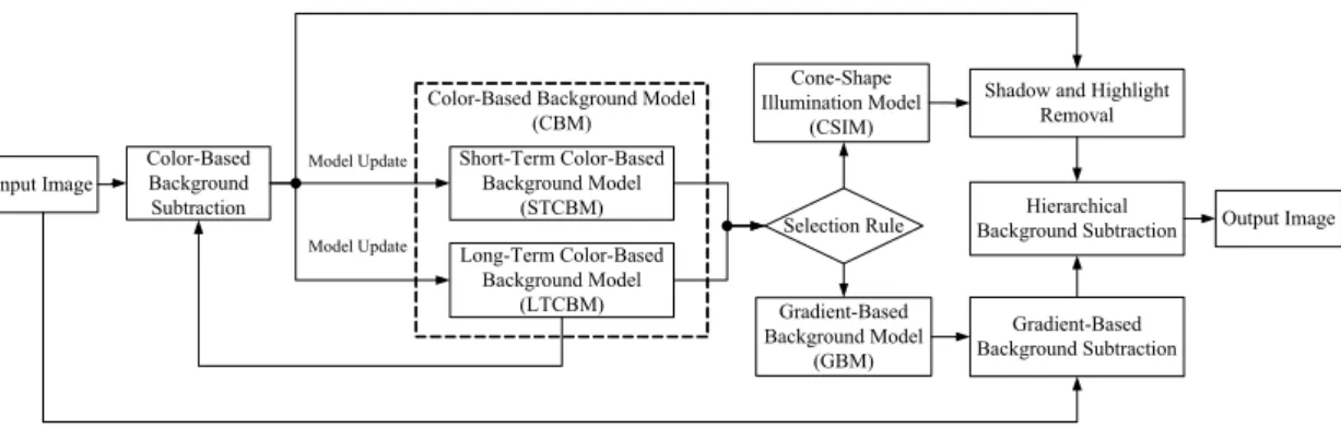
Figure 2-1 illustrates the block diagram of the BSHSR. The BSHSR comprises three main models which are called the CBM, GBM and CSIM. The CBM comprises the LTCBM and STCBM, where the LTCBM is defined to record the background changes during a long period and STCBM is defined to record the background changes during a short period. Moreover, the STCBM and LTCBM are used to determine the parameters of the GBM and CSIM with a selection rule. Four stages are involved in the BSHSR. First, color-based background subtraction is performed on the input image for extracting the foreground candidates via the LTCBM. After that, shadow and highlight removal is performed on the foreground candidates via the CSIM for classifying the pixels of foreground candidates among real foreground, shadow and highlight. For eliminating the false foreground regions, gradient-based background subtraction is performed on the input image via the GBM. Finally, a hierarchal background subtraction is performed for combing the results from the CSIM and GBM.
Color-Based Background Model (CBM) Short-Term Color-Based Background Model (STCBM) Long-Term Color-Based Background Model (LTCBM) Gradient-Based Background Model (GBM) Input Image Color-Based Background Subtraction Gradient-Based Background Subtraction Selection Rule Cone-Shape Illumination Model (CSIM)
Shadow and Highlight Removal Hierarchical Background Subtraction Model Update Model Update Output Image
2.3 Background Modeling
Our previous investigation [56] studied a CBM to record the activity history of a pixel via GMM. However, the foreground regions generally suffer from rapid intensity changes and require a period of time to recover themselves when objects leave the background. In this work, the STCBM and LTCBM are defined and applied to improve the flexibility of the gradient-based subtraction that proposed by Javed
et.al [57]. The features of images used in this work include pixel color and gradient
information. This study assumes that the density functions of the color features and gradient features are both Gaussian distributed.
2.3.1 Color-Based Background Modeling
First, each pixel x is defined as a 3-dimensional vector (R, G, B) at time t. N Gaussian distributions are used to construct the GMM of each pixel, which is described as Eq. (2-1).
∑
= − − ∑ − − ∑ = N i i i T i i d i x x w x f 1 1( )) ) ( 2 1 exp( | | ) 2 ( 1 ) | ( μ μ π λ (2-1)where λrepresents the parameters of GMM,
1 ,..., 2 , 1 , } , , { N 1 i i i i ∑ = = =
∑
= i w and N i w μ λSuppose X ={x1,x2,...,xm} is defined as a training feature vector containing
mpixel values collected from a pixel among a period of m image frames. The next
step is calculating the parameter λ of GMM of each pixel so that the GMM can
λ is the maximum likelihood (ML) estimation. ML estimation aims to find model parameters by maximizing the GMM likelihood function. ML parameters can be obtained iteratively using the expectation maximization (EM) algorithm [58] and the ML estimation of λ is defined as Eq. (2-2).
∑
= = m j j ML f x 1 ) | ( log max arg λ λ λ (2-2)The EM algorithm involves two steps; the parameters of GMM can be derived by iteratively using the Expectation step equation and Maximum step equation, as Eqs. (2-3) and (2-4).
Expectation step: (E step)
1,..., j , ,..., 1 , ) , | ( ) , | ( 1 m N i x f a x f w N k k k j k i i j i ji = = ∑ ∑ =
∑
= μ μ β (2-3) jiβ denotes the posterior probability that the feature xj belongs to the ith
Gaussian component distribution.
Maximum step: (M step)
∑
∑
∑
∑
∑
= = ∧ ∧ ∧ = = ∧ = ∧ − − = ∑ = = m j ji m j T i j i j ji i m j ji m j j ji i m j ji i x x x N w 1 1 1 1 1 / ) )( ( / 1 β μ μ β β β μ β (2-4)The termination criteria of the EM algorithm are as follows:
1. The increment between the new log-likelihood value and the last log-likelihood value is below a minimum increment threshold.
Suppose an image contains S =W×H pixels, where Wmeans the image width
and H means the image height. There are totalS GMMs should be calculated by the
EM algorithm with the collected training feature vector of each pixel.
Moreover, this study uses the K-means algorithm [59], which is an unsupervised data clustering used before the EM algorithm iterations to accelerate the convergence.
First, N random values are chosen from X and assigned as the center of each class.
Then the following steps are applied to cluster the m values of the training feature vector X .
1. To calculate 1-norm distances between the m values and the N center values.
Each value of X is classified to the class having the minimum distance with it. 2. After clustering all the values of X , re-calculate each class center by calculating
the mean of the values among each class.
3. Calculate the 1-norm distances between the m values and the N new center
values. Each value of X is classified to the class which has the minimum distance with it. If the new clustering result is the same as the clustering result before re-calculating each class center, then stop, otherwise return to previous step to calculate the N new center values.
4. After applying K-means algorithm to cluster the values of X , the mean of each
class is assigned as the initial value of μi, the maximum distance among the
points of each class is assigned as the initial value of ∑ , and the value of i w i
2.3.2 Model Maintenance of the LTCBM and STCBM
According to the above sections, an initial color-based probabilistic background model is created using the training feature vector set X with N Gaussian
distributions and N is usually defined as 3 to 5 based on the observation over a
short period of time m. However, when the background changes are recorded over time, it is possible that more different distributions from the original N distributions
are observed. If the GMM of each pixel contains only N Gaussian distributions,
only N background distributions are reserved and other collected background
information is lost and it is not flexible to model the background with only N Gaussian distributions.
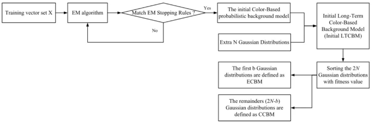
To maintain the representative background model and improve the flexibility of the background model simultaneously, an initial LTCBM is defined as the combination of the initial color-based probabilistic background model and extra N new Gaussian distributions (total 2N distributions), an arrangement inspired by the work of [60]. Kaew et al. [49] proposed a method of sorting the Gaussian
distributions based on the fitness value wi/σi ( ∑i =σi2I ), and extracted a
representative model with a threshold valueB0.
After sorting the first N Gaussian distributions with fitness value, b (b≤N)
Gaussian distributions are extracted with Eq. (2-5).
∑
= > = b j j b B w B 1 0 min arg (2-5) The first b Gaussian distributions are defined as the elected color-based background model (ECBM) to be the criterion to determine the background. Meanwhile, the remainders (2N-b) of the Gaussian distributions are defined as thecandidate color-based background model (CCBM) for dealing with the background changes. Finally, the LTCBM is defined using the combination of the ECBM and CCBM. Figure 2-2 shows the block diagram to illustrate the process of building the initial LTCBM, ECBM and CCBM.
Training vector set X EM algorithm The initial Color-Based
probabilistic background model Match EM Stopping Rules ?
Extra N Gaussian Distributions
Initial Long-Term Color-Based Background Model (Initial LTCBM) Yes No Sorting the 2N Gaussian distributions
with fitness value The first b Gaussian
distributions are defined as ECBM The remainders (2N-b) Gaussian distributions are
defined as CCBM
Figure 2-2 Block diagram showing the process of building the initial LTCBM, ECBM and CCBM.
The Gaussian distributions of the ECBM mean the characteristic distributions of “background”. Therefore, if a new pixel value belongs to any of the Gaussian distributions of the ECBM, the new pixel is regarded as “a pixel contains the property of background” and the new pixel is classified as “background”. In this work, a new pixel value is considered as background when it belongs to any Gaussian distribution in the ECBM and has a probability not exceeding 2.5 standard deviations away from the corresponding distribution. If none of the b Gaussian distributions match the new pixel value, a new test is conducted by checking the new pixel value against the Gaussian distributions in the CCBM. The parameters of the Gaussian distributions are
updated via Eq. (2-6). ρ and α are termed the learning rates , and determine the
update speed of the LTCBM. Moreover, ∧( | t+1)
i t i X
w
p results from background
subtraction which is set to 1 if a new pixel value belongs to the i Gaussian th
distributions in the CBM and the number of Gaussian components in the CCBM is below (2Nb), a new Gaussian distribution is added to reserve the new background information with three parameters: the current pixel value as the mean, a large predefined value as the initial variance, and a low predefined value as the weight. Otherwise, the (2N b− )th Gaussian distribution in the CCBM is replaced by the new
one. After updating the parameters of the Gaussian components, all Gaussian distributions in the CBM are resorted by recalculating the fitness values.
) | ( ) 1 ( 1 1 ∧ + + = − + t i t i t i t i w p w X w α α (2-6) 1 1 (1 ) + + = − + t i t i t i m X m ρ ρ ) ( ) ( ) 1 ( 1 1 1 1 1 + + + + + = − ∑ + − − ∑ t i t i T t i t i t i t i ρ ρ X m X m ) , | ( 1 t i t i t i m X g ∑ =α + ρ
Unlike the LTCBM, the STCBM is defined to record the background changes during a short period. Suppose B1 frames are collected during a short period B1 and then B1 new incoming pixels for each pixel are collected and defined as a test pixel
set
{
}
1 ,..., ,..., , 2 1 p pq pB pP = , where pq means the new incoming pixel at time q.
A test pixel set P is defined and used for calculating the STCBM and a result set S
is then defined and calculated by comparing P with the LTCBM and is described as
Eq.(2-7), where I means the result after background subtraction ,which means the q
index of Gaussian distribution of the initial LTCBM, R means the index of q
resorting result for each Gaussian distribution after each update, and F means the q
{
1, ,..., ,...,2 q B1`, q ( , ( ), ( ))q q q}
S= S S S S and S = I R i F i (2-7) where 1≤ ≤Iq 2 , 1N ≤R iq( ) 2 , ( ) {0,1},1≤ N F iq ∈ ≤ ≤i 2N
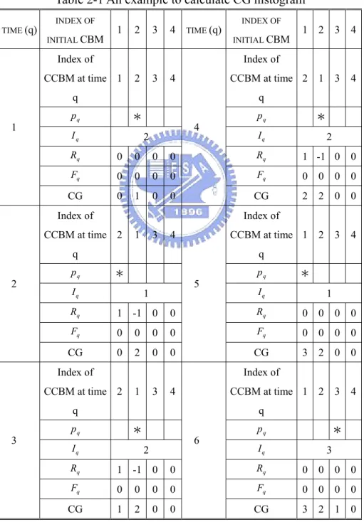
The histogram of CG is then given using Eq. (2-8).
' ' ' _ 1 ( ) [ ( ( ( ))) ( ( ( )))]/ CG k q q q q q q q q H k =
∑
δ k− I +R I + ⋅F∑
δ k− I +R I B (2-8) where ' 1 1≤ ≤k 2 , 1N ≤ ≤q B,1≤ < q qIn brief, four Gaussian distributions are used to explain how Eqs. (2-7) and (2-8) work and the corresponding example is listed in Table 2-1. At first, the original CBM contains four Gaussian distributions (2N =4), and the index of Gaussian distribution in the initial CBM is fixed (1,2,3,4). At the first time, a new incoming pixel which belongs to the second Gaussian distribution compares with the CBM, so the result of
background subtraction is Iq =2. Moreover, the CBM is updated with Eq. (2-6) and
the index of Gaussian distribution in the CBM is changed. When the order of the first and second Gaussian distributions is changed, Rq(i) records the change states; for example, 1Rq(1)= means the first Gaussian distribution has moved forward to the
second one, and Rq(2)=−1 means the second Gaussian distribution has moved
backward to the first one. At the second time, a new incoming pixel which belongs to the second Gaussian distribution based on the initial CBM is classified as the first Gaussian distribution (Iq =1) based on the latest order of the CBM. However, the CG histogram can be calculated according to the original index of the initial CBM with the latest order of the CBM and Rq(i), such that HCG(Iq +Fq =2) will be
distributions changes. For example, at the fifth time in Table 2-1, the order of CBM changes from (2,1,3,4) to (1,2,3,4), and then Rq(1)=1−1=0 means the first Gaussian distribution of the initial CBM has moved back to the first one of the latest CBM, and Rq(2)=−1+1=0means the second Gaussian distribution has moved back to the second one of the latest CBM.
Table 2-1 An example to calculate CG histogram
TIME (q) INDEX OF INITIAL CBM 1 2 3 4 TIME (q) INDEX OF INITIAL CBM 1 2 3 4 Index of CCBM at time q 1 2 3 4 Index of CCBM at time q 2 1 3 4 q p * pq * q I 2 Iq 2 q R 0 0 0 0 Rq 1 -1 0 0 q F 0 0 0 0 Fq 0 0 0 0 1 CG 0 1 0 0 4 CG 2 2 0 0 Index of CCBM at time q 2 1 3 4 Index of CCBM at time q 1 2 3 4 q p * pq * q I 1 Iq 1 q R 1 -1 0 0 Rq 0 0 0 0 q F 0 0 0 0 Fq 0 0 0 0 2 CG 0 2 0 0 5 CG 3 2 0 0 Index of CCBM at time q 2 1 3 4 Index of CCBM at time q 1 2 3 4 q p * pq * q I 2 Iq 3 q R 1 -1 0 0 Rq 0 0 0 0 q F 0 0 0 0 Fq 0 0 0 0 3 CG 1 2 0 0 6 CG 3 2 1 0
If a new incoming pixel p matches the q i Gaussian distribution that has the th
least fitness value, the i Gaussian distribution is replaced with a new one and the th
flag F will be set to 1 to reset the accumulated value of q HCG(i). Figure 2-3 shows the block diagram about the process of calculatingH . CG
No
Test Pixel Pq Color-based Background
Subtraction q=B1? Calculate HCG
q=q+1 Resorting the Gaussian
Distributions of the LTCBM The result structure Sq of the
background Subtraction
Yes
LTCBM
Record Sq into the result structure S
Figure 2-3 Block diagram showing the process to calculate H . CG
After matching all test pixels to the corresponding Gaussian distribution, the result set S can be used to calculating H using CG I and q F . With the reset flag q F , q
the STCBM can be built up rapidly based on a simple idea, threshold on the occurring frequency of Gaussian distribution. That is to say, the short-term tendency of
background changes is apparent if an element ofHCG(k) is above a threshold
valueB2 during a period of frames B1. In this work, B1 is assigned a value of 300
frames and B2 is set to be 0.8. Therefore, the representative background component
in the short-term tendency can be determined to be k if the value of HCG(k)
exceeds 0.8, otherwise, the STCBM provides no further information on background model selection.
2.3.3 Gradient-Based Background Modeling
Javed et.al [57] developed a hierarchical approach that combines color and
gradient information to solve the problem about rapid intensity changes. Javed et.al
obtain the gradient information to build the gradient-based background model. The choice of k in [57] is similar to select k based only on the ECBM defined in this work. However, choosing the highest weighted Gaussian component of GMM leads to the loss of the short term tendencies of background changes. Whenever a new Gaussian distribution is added into the background model, it is not selected owing to its low weighting value for a long period of time. Consequently, the accuracy of the gradient-based background model is reduced for that the gradient information is not suitable for representing the current gradient information.
To solve this problem, both STCBM and LTCBM are considered in selecting the value of k for developing a more robust gradient-based background model and maintaining the sensitivity to short-term changes. When the STCBM provides a
representative background component (says the th
s
k bin in the STCBM), k is set to
s
k rather than the highest weighted Gaussian distribution.
Let xt, [R,G,B]
j
i = be the latest color value that matched the
th s
k distribution of
the LTCBM at pixel location( ji, ), then the gray value of t j i
x, is applied to calculate
the gradient-based background subtraction. Suppose the gray value of t
j i
x, is
calculated as Eq. (2-9), then t
j i
g, will be distributed as Eq. (2-10) based on
independence among RGB color channels,
B G R gt j i, =α +β +γ (2-9) ) ) ( , ( ~ 2 , , , t j i t j i t j i N m g σ (2-10) where B k t j i G k t j i R k t j i t j i s s s m , , , , , , , , , , =αμ +βμ +γμ
2 , , , 2 2 , , , 2 2 , , , 2 , ( ) ( ) ( ) B k t j i G k t j i R k t j i t j i α σ s β σ s γ σ s σ = + +
After that, the gradient along the x axis and y axis can be defined as
t j i t j i x g g f = +1, − , and t j i t j i y g g
f = , +1− , . From the work of [57], f and x f have the y
distributions defined in Eqs. (2-11) and (2-12). ) ) ( , ( ~ 2 x x f f x N m f σ (2-11) ) ) ( , ( ~ 2 y y f f y N m f σ (2-12) where t j i t j i f m m m x = +1, − , t j i t j i f m m m y = , +1 − , 2 , 2 , 1 ) ( ) ( t j i t j i fx σ σ σ = + + 2 , 2 1 , ) ( ) ( t j i t j i fy σ σ σ = + + Suppose 2 2 y x m = f + f
Δ is defined as the magnitude of the gradient for a pixel,
) / ( tan 1 y x d f f − =
Δ is defined as its direction (the angle with respect to the
horizontal axis), and Δ =
[
Δm,Δd]
is defined as the feature vector for modeling the gradient-based background model. The gradient-based background model based on feature vector Δ =[
Δm,Δd]
then can be defined as Eq. (2-13).(
)
k g f k f d m k z T F y x > ⎟⎟ ⎠ ⎞ ⎜⎜ ⎝ ⎛ − − − ∏ Δ = Δ Δ ) 1 ( 2 exp 1 2 , 2 2 m ρ ρ σ σ (2-13) where2 2 sin sin cos 2 cos ⎟ ⎟ ⎠ ⎞ ⎜ ⎜ ⎝ ⎛Δ Δ − + ⎟ ⎟ ⎠ ⎞ ⎜ ⎜ ⎝ ⎛Δ Δ − ⎟ ⎟ ⎠ ⎞ ⎜ ⎜ ⎝ ⎛Δ Δ − − ⎟ ⎟ ⎠ ⎞ ⎜ ⎜ ⎝ ⎛Δ Δ − = y y y y x x x x f f d m f f d m f f d m f f d m z σ μ σ μ σ μ ρ σ μ y x f f t j i σ σ σ ρ = ( , )2
2.4 Background Subtraction with Shadow Removal
2.4.1 Shadow and Highlight Removal
Besides foreground and background, shadows and highlights are two important phenomenons that should be considered in most cases. Shadows and highlights result from changes in illumination. Compared with the original pixel value, shadow has similar chromaticity but lower brightness, and highlight has similar chromaticity but higher brightness. The regions influenced by illumination changes are classified as the foreground if shadow and highlight removal is not performed after background subtraction.
Hoprasert et al. [60] proposed a method of detecting highlight and shadow by gathering statistics from N color background images. Brightness and chromaticity distortion are used with four threshold values to classify pixels into four classes. The method that used the mean value as the reference image in [60] is not suitable for dynamic background. Furthermore, the threshold values are estimated based on the histogram of brightness distortion and chromaticity distortion with a given detection rate, and are applied to all pixels regardless of the pixel values. Therefore, it is possible to classify the darker pixel value as shadow. Furthermore, it cannot record the history of background information.
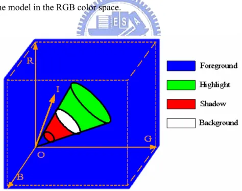
This work proposes a 3D cone model that is similar to the pillar model proposed by Hoprasert [60], and combines the LTCBM and STCBM to solve the above problems. A cone model is proposed with the efficiency in deciding the parameters of 3D cone model according to the proposed LTCBM and STCBM. In the RGB space, a Gaussian distribution of the LTCBM becomes an ellipsoid whose center is the mean of the Gaussian component, and the length of each principle axis equals 2.5 standard
deviations of the Gaussian component. A new pixel I(R,G,B) is considered to
belong to background if it is located inside the ellipsoid. The chromaticities of the pixels located outside the ellipsoid but inside the cone (formed by the ellipsoid and the origin) resemble the chromaticity of the background. The brightness difference is then applied to classify the pixel as either highlight or shadow. Figure 2-4 illustrates the 3D cone model in the RGB color space.
Figure 2-4 The proposed 3D cone model in the RGB color space.
The threshold values τlow and τhigh are applied to avoid classifying the darker pixel value as shadow or the brighter value as highlight, and can be selected based on the standard deviation of the corresponding Gaussian distribution in the CBM.
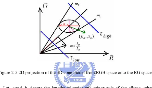
Because the standard deviations of the R, G and B color axes are different, the angles between the curved surface and the ellipsoid center are also different. It is difficult to classify the pixel using the angles in the 3D space. The 3D cone is projected onto the 2D space to classify a pixel using the slope and the point of tangency. Figure 2-5 illustrates the projection of the 3D cone model onto the RG 2D space.
Figure 2-5 2D projection of the 3D cone model from RGB space onto the RG space. Let a and b denote the lengths of major and minor axis of the ellipse, where
R
a=2.5*σ and b=2.5*σG. The center of the ellipse is (μR,μG), and the elliptical equation is described as Eq. (2-14).
1 ) ( ) ( 2 2 2 2 = − + − b G a R μR μG (2-14)
The line G=mR is assumed to be the tangent line of the ellipse with the slope
m. Equation (2-10) can then be solved using the line equation G=mR with
Eq.(2-15). ) ( 2 ) )( 2 ( 4 ) ( ) 2 ( 2 2 2 2 2 2 2 2 , 1 R G G R R G R a b a m μ μ μ μ μ μ μ − − − − ± − = (2-15)
A matching result set is given by Fb =
{
fbi,i=1,2,3}
, where f is the matching biresult of a specific 2D space. A pixel vectorI =
[
IR,IG,IB]
is then projected onto the 2D spaces of R-G, G-B, and B-R. The pixel matching result is set to 1 when the slopeof the projected pixel vector is between m1 and m . Meanwhile, if the background 2
mean vector is E =
[
μR,μG,μB]
, the brightness distortion αb can be calculated via Eq. (2-16) || || ) cos( || || E I b θ α = (2-16) where 1 1 2 2 2 2 cos ( G ) cos ( G ) I E R G R G I I I μ θ θ θ μ μ − − = − = − + +The image pixel is classified as highlight, shadow or foreground using the matching result set F , the brightness distortion b αb and Eq. (2-17).
⎪ ⎩ ⎪ ⎨ ⎧ < < = < < = =
∑
∑
: , 1 and 3 : ighlight , 1 and 3 : hadow ) ( C b high b low otherwise Foreground else F H else F S i b b τ α α τ (2-17)When a pixel is a large standard deviation away from a Gaussian distribution, the Gaussian distribution probability of the pixel approximately equals to zero. It also means the pixel does not belong to the Gaussian distribution. By using the simple
concept, τhigh and τlow can be chosen using N standard deviation of the G
|| || cos || || 1 || || cos || || 1 low high E S E S τ τ θ τ θ τ ⋅ − = ⋅ + = (2-18) where
( ) ( )
2 2 || ||E = μR + μG(
) (
2)
2 G G || ||S = N ⋅σR + N ⋅σG 1 1 2 2 2 2 cos ( G ) cos ( G ) E S R G R G τ μ σ θ θ θ μ μ σ σ − − = − = − + + 2.4.2 Background SubtractionA hierarchical approach combining color-based background subtraction and gradient-based background subtraction has been proposed by Javed et.al [57]. This work proposes a similar method for extracting the foreground pixels. Given a new image frame I , the color-based backgound model is set to the LTCBM and STCBM,
and gradient-based model is Fk
(
Δ ,m Δd)
. C(I) is defined as the result ofcolor-based background subtraction using the CBM. G(I) is defined as the result of gradient-based background subtraction. C(I) and G(I) can be extracted by testing every pixel of frame I using the LTCBM and Fk
(
Δ ,m Δd)
. Moreover, C(I) and) (I
G are both defined as a binary image, where 1 represents the foreground pixel
and 0 represents the background pixel. The foreground pixels labeled in C(I) are
further classified as shadow, highlight and foreground by using the proposed 3D cone model. C'(I) can then be obtained from C(I) after transferring the the foreground
background pixel. The difference between Javed et.al [57] and the proposed method is that a pixel classifying procedure using the CSIM is applied before using the connected component algorithm to group all the foreground pixels in C(I ). The robustness of background subtraction is enhanced due to the better accuracy in |∂Ra |. Moreover, the foreground pixels can be extracted using Eq. (2-19).
B a R j i P R j i G j i I a ≥ ∂ ∇
∑
∈∂ | | )) , ( ) , ( ( ) , ( (2-19)where I∇ denotes the edges of image I and ∂ represents the number of Ra
Chapter 3
Incremental Similarity-Based
Aspect-Graph 3D Object Recognition
3.1 Introduction
The common challenge in 3D object recognition, human posture recognition, and scene recognition is the variation in orientations. The simplest method for solving this problem is to characterize an object with a densely sampled collection of independent views. The object can be described in detail by constructing an object model with numerous 2D views; however, this approach significantly increases computing time due to the expansive search space. Thus, several approaches have been developed to extract a minimal set of object views. Appearance-based methods focus on changes in intensity of each view. However, changes to object lighting, rotation, deformation and occlusion affect object recognition results when using the appearance-based method. Aspect-graph representations focus on shape changes to an object’s projection [61-62]. Koenderink et al. [63] developed the underlying theory that describes 3D objects
![Table 4-3 The comparison between the proposed method and that proposed by Hoprasert [60] via global illumination changes with fluorescent lamps](https://thumb-ap.123doks.com/thumbv2/9libinfo/8106985.165391/67.892.126.769.756.1010/table-comparison-proposed-proposed-hoprasert-illumination-changes-fluorescent.webp)
