國
立
交
通
大
學
資訊科學與工程研究所
碩
士
論
文
在無線隨意網路下利用功率調整增進網路流量的
機制
A Novel MAC Layer Power Control Protocol for Throughput
Enhancement in Wireless Ad Hoc Networks
研 究 生:吳松燊
中 華 民 國 九 十 八 年 七 月
在無線隨意網路下利用功率調整增進網路流量的機制
A Novel MAC Layer Power Control Protocol for Throughput Enhancement in Wireless Ad Hoc Networks
研 究 生:吳松燊 Student:Sung-Shen Wu
指導教授:趙禧綠 Advisor:Hsi-Lu Chao
國 立 交 通 大 學
資 訊 科 學 與 工 程 研 究 所
碩 士 論 文
A ThesisSubmitted to Department of Computer and Information Science College of Electrical Engineering and Computer Science
National Chiao Tung University in partial Fulfillment of the Requirements
for the Degree of Master
in
Computer and Information Science July 2009
Hsinchu, Taiwan, Republic of China
i
摘 要
在無線隨意網路上傳輸資料功率調整對增加整個網路流量相當有潛力,在現存 的傳輸資料功率調整的方法中,大多數的方法都是使用多條頻寬及多個收發器。 但是使用多條頻寬跟多個收發器不僅比較浪費頻道資源也會增加硬體花費的費 用。 在這篇論文中我們提出一個創新功率控制的演算法使用單條頻道及單個收發 器去增加整個網路的流量。我們將IEEE 802.11 控制層下的演算法做修改,我們 並不使用最大的功率傳輸封包,而是依照頻道的品質動態的去調整傳輸封包。此 外當節點要傳輸資料時並不用等到頻道沒有人使用才能傳輸,使得我們在同一時 間多個節點可以同時進行傳輸。所以頻道利用率及網路流量都因此而上升。此外 因為調整功率大小可能會有隱藏節點的問題產生,在我們的演算法中我們也有考 慮到隱藏節點的問題。而在模擬的結果顯示出我們的演算法成功的增加網路的流 量。ii
Abstract
Transmission power control (TPC) has great potentials to increase throughputs of a mobile ad hoc network (MANET). Among existing TPC protocols, most of them can achieve throughputs by using multiple channels and multiple transceivers. Using multiple channels and transceivers is not only wasting resources but also increasing hardware costs.
In this thesis, we present a novel power controlled MAC protocol which uses a single-channel and a single-transceiver to increase network throughputs by modifying IEEE 802.11 MAC layer protocol. Instead of using a maximum power to transmit RTS and CTS, our protocol uses an adaptive power which based on a channel quality information to transmit data. Since our protocol allows multiple pairs concurrently transmitting data, we can improve spatial reuses and the throughputs in networks. We also consider hidden terminal problems. The performance evaluation is shown that our protocol successfully increases network throughputs. The performance of our protocol is better than the POWMAC protocol and IEEE 802.11 protocol.
iii
致 謝
本論文得以順利的完成,首先感謝指導教授的--趙禧綠教授悉心指導,在這 兩年研究論文中,老師提供了許多相當寶貴的意見,並且課業上給予相當大的幫 助,針對論文不足之處也能迅速的給予建議,使我們能一步步完成並且順利畢 業;從一開始決定論文的題目開始到最後的論文撰寫,中間所要經歷的過程是以 前從來沒有經驗過的,經由老師的耐心指導下論文也漸漸有了雛形。非常謝謝趙 老師給我的指導與關心 接者要感謝的是我的實驗室同學們,在研究期間實驗室同學們之間互相討 論、勉勵相持,在我心情不好時陪我聊天,在我有疑問時給我解答,在他們的陪 伴下更能認真迅速的完成論文。與老師以及實驗是同學們度過兩年的碩士生涯, 獲益良多,很感謝他們造就我的進步以及帶給我一段很豐富的人生 最後要感謝的是我的家人,碩士學位順利的完成得自於爸爸、媽媽無怨無悔 的付出與關懷,讓我在大學畢業後還可以繼續唸書深造,以及感謝 cub 和 pukii 的陪伴,在此將所有的喜悅與榮耀與他們共享。iv
Contents
摘 要 ... i Abstract ... ii 致 謝 ... iii Contents ... ivList of Tables ... vi
List of Figures ... vii
Chpater 1 Introduction ... 1
1.1 Transmission power control in IEEE 802.11 protocol ... 3
1.2 Power control issues ... 3
1.3 Objectives ... 5
1.4 Organization ... 6
Chpater 2 Related Work ... 7
2.1 Transmission power control in multiple channels ... 7
2.2 Transmission power control in a single channel ... 8
Chpater 3 Proposed MAC Protocol ... 12
3.1 Assumption ... 12
3.2 Parameters and control frames ... 13
3.3 Neighbor tables ... 14
3.4 The proposed protocol ... 14
3.5 Hidden terminals problems ... 24
3.6 Contention resolution ... 27
3.7 Peroformance analysis ... 29
v 4.1 Environment setting ... 34 4.2 Scenario one ... 35 4.3 Scenario two... 37 4.4 Scenario three... 38 4.5 Scenario four ... 43
Chpater 5 Conclusion and Future Work ... 45
vi
List of Tables
Table 3 - 1 List of notations ... 13 Table 4 - 1 Simulation and analysis parameters………...34
vii
List of Figures
Figure 1 - 1 The expose terminal problem ... 3
Figure 3 - 1 Example of our protocol (1)……….21
Figure 3 - 2 Example of our protocol (2) ... 21
Figure 3 - 3 Example of our protocol (3) ... 22
Figure 3 - 4 Example of our protocol (4) ... 22
Figure 3 - 5 Example of our protocol (5) ... 23
Figure 3 - 6 The basic operation of the protocol ... 23
Figure 3 - 7 The flow chart of our protocol ... 24
Figure 3 - 8 Hidden terminals problem. ... 25
Figure 3 - 9 Example of nodes relay CTS in our protocol (1) ... 26
Figure 3 - 10 Example of nodes relay CTS in our protocol (2) ... 26
Figure 3 - 11 Example of nodes use probability Pr to transmit RTS ... 27
Figure 3 - 12 An illustrative example of proposed contention resolution... 28
Figure 3 - 13 A time diagram of a packet transmission time ... 33
Figure 4 - 1 A Line topology for scenario one……….36
Figure 4 - 2 Throughputs in the scenario one ... 36
Figure 4 - 3 The topology of scenario two ... 37
Figure 4 - 4 Throughputs in the scenario two ... 38
Figure 4 - 5 Throughputs in the scenario three ... 40
Figure 4 - 6 Throughputs of different speeds ... 41
Figure 4 - 7 Energy consumption in different scenarios ... 41
Figure 4 - 8 Energy consumption per packet in different scenarios ... 42
viii
Figure 4 - 10 Energy consumption in different scenario ... 43
Figure 4 - 11 Energy consumption per Kbps in different scenario ... 43
Figure 4 - 12 The topology to show the effect of relaying CTS ... 44
1
Chpater 1 Introduction
A mobile ad hoc network (MANET) has become very popular in a modern society due to its easy and quick deployment with low cost. We can easily access an Internet through mobile ad hoc network in almost everywhere. MANET technology uses IEEE 802.11 standard [1-3]. In a mobile ad hoc network, users exchange their information to their destinations without using an access point (AP) and the channel is shared by all nodes. Sometimes more than one node will try to transmit data concurrently, and collisions will occur. In IEEE 802.11 specification, a medium access control (MAC) protocol is defined to coordinate concurrent transmissions and avoid collisions.
In order to coordinate multiple transmissions at one channel, IEEE 802.11 MAC layer protocol utilizes a four-way handshake to resolve the problem. When a node wants to transmit data to another terminal, sender first transmits a request-to-send (RTS) packet to a receiver. When a receiver receives RTS, it replies back using a clear-to-send (CTS) packet. When a sender receives CTS, it can start to transmit data, and once complete, a receiver transmits back an acknowledgement (ACK) packet to a sender. RTS and CTS packets include duration of data transmission time. Other terminals overhearing RTS or CTS defer their transmissions until the ongoing transmissions finished. CTS is used to avoid collisions occurring at a receiver side, while RTS message is to prevent collisions at a sender side. Terminals transmit their control and data packets at a maximum power level. All current transmissions can avoid collisions through a four-way handshake method.
2
coordinate current transmissions without collisions, the problem which we called expose terminal problem may still happen.
Nodes overhearing RTS and CTS defer their transmissions until ongoing transmissions are finished. However, some nodes can transmit data without distrupt ongoing pairs. They just need to select an approximate power to transmit data. For example, nodes A and B are exchanging data as shown in Fig.1-1. . It is obvious nodes D and E cannot transmit data simultaneously to avoid interfering nodes A and B. Since nodes C and E are in RTS and CTS range, they set a network allocation vector (NAV) to wait a channel clear. The dashed circles indicate the maximum transmission ranges, while the dotted ones indicated the ranges of the minimum transmission ranges. Nodes D and E can’t transmit any data to nodes C and F even they won’t distribute the ongoing transmission between nodes A and B. The problems are called expose terminal problems. It is easy to show that the three transmissions can transmit data concurrently when they select their transmission power appropriately. IEEE 802.11 MAC layer protocol can’t dynamically adjust nodes transmission power, even if a position of a sender and a receiver is very close. Expose terminal problems will waste bandwidths and reduce throughputs in a network. In the next section, we introduce a transmission power control method in IEEE 802.11 MAC layer protocol.
3
Figure 1 - 1 The expose terminal problem
1.1 Transmission power control in IEEE 802.11 protocol
IEEE 802.11 standard specifies a MAC layer protocol including distributed coordination function (DCF) and point coordination function (PCF). In IEEE 802.11 MAC layer protocol, wireless nodes have two power modes: ongoing transmission and power saving (PS). The power management scheme divides time into beacon intervals. At a beginning of each beacon interval, power saving nodes wake up for a short time period, called announcement traffic indication message (ATIM) window. In the ATIM window, nodes exchange control frames, called ATIM frames, to inform their power saving counterparts to remain awake until the end of the beacon interval to receive data frames. After ATIM window, all nodes follow a DCF protocol using maximum power to transmit their data frames.
1.2 Power control issues
One of main targets in designing mobile ad hoc networks (MANET) is how to enhance overall networks throughputs while maintaining low energy consumption for packet processing and communications. In power control schemes, there are two
4
major issues we often discussed. One is using power control scheme to reduce an energy consumption, and the other one is to reduce interferences to other nodes to increase network throughputs.
First we introduce reducing energy issues. Since IEEE 802.11 MAC layer protocol always uses maximum power to transmit packets, it wastes a lot of energy, and it is based on the carrier sense multiple access with collision avoidance (CSMA/CA) medium access procedure to transmit/receive both control and data frames. We know that CSMA/CA wastes the scarce energy and bandwidth due to frame collisions and lengthens the transmission delay due to waiting backoff time, especially in heavy traffic load. In addition, the IEEE 802.11 power management scheme does not specify how to determine the ATIM window size in a beacon interval. The fixed ATIM window size cannot always accommodate the dynamically changing traffic conditions. Using power control to reduce the energy consumption has become a popular issue.
Second we introduce increasing network throughputs issues. According to IEEE 802.11 MAC layer protocol, one node overhearing RTS or CTS needs to set NAV and keeps silent to avoid collisions occur. IEEE 802.11 MAC layer protocol uses a maximum transmission power for all nodes to transmit control and data packets, no matter how close a transmitter to its intended receiver. In IEEE 802.11 MAC layer protocol, since nodes always use maximum power to transmit packets, energy is used inefficiently and spatial reuses and throughputs in networks are low. Transmission power control is a technique for increasing the efficiency of space-time utilization in wireless networks. Generally speaking, reducing transmission power results less interferences to nearby transceivers and receivers. Therefore, more transmissions can be activated simultaneously, improving the overall throughputs of the network.
5
In this paper, we focus on a reduce interferences to nearby transceivers and receivers to increase an overall network throughputs.
Some literature increases network throughputs by using multiple channels and multiple transceivers. [4-5] use a control channel to communicate channel quality information, and based on channel quality information a terminal can select an appropriate power to transmit data. However, using control channel may add more hardware cost and more difficult to implement. Therefore, recent researches [6-10], use a single channel and a single transceiver instead of multiple channels and multiple transceivers. We will discuss them in the chapter 2. Since using a single channel and a single transceiver can reduce a hardware cost than using multiple channels and multiple transceivers, we propose a power management protocol in a single channel and a single transceiver environment. We modify IEEE 802.11 MAC layer protocol. Besides, we also consider hidden terminal problems and mobility issues in the chapter 3.
1.3 Objectives
In IEEE 802.11 medium access control layer, nodes can transmit data only in sensing channel idle. As we described before, since nodes in IEEE 802.11 MAC layer protocol always use a maximum power to transmit data, they cannot dynamically adjust their transmission power. One node overhearing RTS and CTS defers its data transmission and avoids collisions. That will cause the expose terminal problem. In IEEE 802.11 MAC layer protocol, it can’t allow concurrent transmissions, and one node wants to transmit data needs to wait a channel clear. Spatial reuses and throughputs are very low. In IEEE 802.11 physical layer (PHY), nodes can correct
6
decode packets when signal to noise ratio (SNR) reaches a threshold. We combine the packets decode threshold in PHY and sensing channel clear data transmission in MAC layer. We modify IEEE 802.11 MAC protocol based on SNR threshold in PHY layer.
In order to increase throughputs and spatial reuses, we propose a novel MAC layer protocol based on SNR threshold in PHY layer to increase channels utilization. We propose a new adaptive transmission power control protocol which can improve the network throughputs significantly using a single channel and a single transceiver. Specifically, by controlling the transmission power, our protocol can enable several concurrent transmissions without interfering with each other. Since adjust minimum power may cause hidden terminal problems, and most power control protocols doesn’t consider them. In our protocol, we relay CTS to avoid hidden terminal happened.
According to our protocol, nodes can dynamically adjust their transmission power without distributing ongoing pairs. Dissimilar to IEEE 802.11 MAC layer protocol, we allow multiple pairs currently transmit data, thus nodes don’t need to set NAV when sensing channels being busy, and we also don’t need to use extra messages and synchronize data transmission.
1.4 Organization
The organization of this thesis is as follow: In chapter 2, we review related work of transmission power control. Then our protocol will be described in chapter 3. The performance evaluation will be shown and discuss in chapter 4. In the end, chapter 5 will be the conclusion.
7
Chpater 2 Related Work
Some literals use multiple channels environment to design a transmission power control protocol and some literals use a single channel. In multiple channels power control protocol, nodes exchange channel quality information in a control channel and exchange data packets in a data channel. Since it using multiple channels, nodes can concurrently exchange channel quality information and data, and use an appropriate power to transmit data based on channel quality information. Single channel power control protocol uses only one channel instead of multiple channels to exchange channel quality information. Nodes do not use control channels to exchange channel quality information. Since they use only one channel, they can reduce hardware costs and easier to implement. In the section 2.1 and 2.2, we will discuss related works of power control protocol in multiple channels and a single channel environment.
2.1 Transmission power control in multiple channels
Some papers increase the network throughput by using multiple channels and multiple transceivers. Nodes can exchange channel quality information and data concurrently.
Jeffrey P. Monks, Vaduvur Bharghavan, and Wen-mei W. Hwu [4] propose a power controlled multiple access (PCMA) protocol to improve a network throughput. In PCMA protocol, they use two channels. One is used to send the control message called control channel, and the other is used to transmit data. The sender broadcast the packet to exchange channel quality information of the ongoing transmission nodes in
8
the control channel. Base on the channel quality information of the ongoing transmission nodes, the sender can select an appropriate power for data transmission, and avoid the collision. However, using multi-channels and multi-transceivers introduces additional hardware cost and implementation complexity. The PCMA protocol considers the fix modes topology, and it doesn’t consider movement of nodes.
Alaa Muqattash and Marwan Krunz [5] propose power controlled dual channel
medium access protocol (PCDC) to improve network throughputs. PCDC uses two channels environment in power control protocol. One is for data transmission and the other is for channel quality information. When one node wants to find its next hop, it will consider the channel quality between it and its receiver. The node will choose the next hop which is in good channel quality. PCDC has the same problem like PCMA. Using multi-channel and multi-transceiver introduces additional hardware cost and implementation complexity.
2.2 Transmission power control in a single channel
Some papers increase the network throughputs by using a single channel and a single transceiver. It can not only reduce the additional hardware cost but also reduces implementation complexity.
Muqattash and Krunz [6] propose a throughput oriented MAC layer protocol utilizing a single channel and a single transceiver, called power controlled protocol (POWMAC). POWMAC uses a new decision rule: when a node overhears other nodes’ transmissions, it is still allowed to carry out its own data transmission as long as it does not interfere with the ongoing ones. Nodes in POWMAC exchange their
9
control message in a period mean Access Window (AW) window. They create a new packet mean “DTS” to synchronize data transmission. When nodes receive DTS, they can’t transmit data immediately. After AW window time finished, they transmit data simultaneously. Thus, according to POWMAC, several transmissions can transmit data concurrently. However, POWMAC cannot gain dramatic improvement on network throughput due to the following three reasons. First, POWMAC needs the Access Window (AW) window to synchronize the data transmission, so it will cause serious delay times for each pair. Second, several concurrent DATA transmissions may not take place if they are not synchronized due to the existence of propagation delay. Third, POWMAC can’t dynamically adjust the AW window size. Even if a network has light traffic, nodes still need to wait the AW window finished.
Alawieh, Assi and Ajib [7] propose Directional MAC protocol (D-MAC) in a single channel and a single transceiver environment. D-MAC uses the direction antennas instead of the omni-antennas. They define two interferences areas. One is the potential interfere area, and the other one is the indirect interfere area. In the potential area, nodes may turn their directional antenna in any direction. In the indirect interfere area, nodes will not cause any direct interference. They calculate interferences of the potential interferes area and the indirect interfere area. By calculating around interferences, nodes can use appropriate power to transmit data. Although D-MAC calculates around interferences that a sender can use appropriate power to transmit data, it doesn’t consider the appropriate power may disrupt the ongoing pairs.
Swades De, Komlan Egoh and Gaurav Dosi [8] propose an enhanced receiver initiated power control multi-access protocol (E-RIMA) for throughput enhancement. In E-RIMA protocol, senders use the maximum power to transmit the RTS and the
10
CTS message, and use a minimum power to transmit data. Since nodes use minimum power to transmit data, some nodes in the interfering area cannot sense the channel busy. They may use maximum power to transmit the RTS message. The collisions will happen. That will cause the hidden terminal problem. In order to solve this problem, the receiver will period send the busy tone to avoid this problem, and receiver’s neighbors can estimate their channel gain from the receiver by the busy tone. Based on the busy tone, the neighbors can use the appropriate power to transmit data without interfere ongoing transmission pairs. However, in E-RIMA protocol, the receiver needs to period send the busy tone. Senders must stop the data transmission to match up with receivers, and need to synchronize with the receiver. It will reduce the throughput and waster a lot of power for receiver to send the busy tone.
Kuei-Ping Shih, Chau-Chieh Chang and Yen-Da Chen [9] propose a fragmentation based protocol with power control (F-RCRC) for throughput enhancement. F-RCRC protocol uses maximum power to transmit control message and minimum power to transmit data. When nodes use minimum power to transmit data, hidden terminal problems may happen. Although in IEEE 802.11 nodes will set EIFS to wait the channel clear, EIFS is too short for the long frames transmission. Segmenting long frame will increase packets overhead. Since EIFS is too short for long frames transmission, nodes cannot detect the nearby ongoing transmission nodes. It may cause hidden terminal problems. F-RCRC calculates FIFS instead of EIFS. The duration of FIFS is longer than EIFS such that the number of fragments that a long frame is fragmented can be reduced. Since F-RCRC is still under the 802.11 protocol, nodes overhearing RTS and CTS packets can’t send any data.
11
Power Control protocol (FAIR) that uses power control scheme to solve the fairness problem. They dynamically adjust the contention window size (CWs). Using large power to transmit control message has less number of hidden terminal nodes than using small power. When nodes use a small power to send data, FAIR protocol sets less contention window sizes to increase a probability of transmitting data. Nodes use a larger power to transmit data, and they set the large contention window sizes to reduce a probability of transmitting data. Although FAIR protocol can exactly enhance a fairness of different pairs, it can’t increase throughputs of overall networks.
12
Chpater 3 Proposed MAC Protocol
In this chapter, we propose a novel Mac layer protocol to enhance throughputs in a single channel and a single transceiver environment. According to IEEE 802.11 MAC protocol, every node has to carry the physical carrier sensing before transmitting RTS, CTS, or DATA packets. If the channel is sensed to be busy, then the nodes cannot transmit those packets. As a result, the spatial reuse is very low because each time the channel can be used by only one pair of transmitter and receiver.
In this essay, we modify IEEE Mac layer protocol in a single channel and a single tranceiver environment to increase throughputs based on SNR threshold in PHY.Our protocol does not use any new control packets other than RTS and CTS. Specifically, in our protocol, nodes that overhear RTS or CTS can make a decision on whether they can transmit data packets to their intended receivers based on some useful information carried by RTS/CTS.
In the following section, first we discuss an assumption of our protocol. Second we show parameters and control frame which used in our protocol. Third, we introduce a neighbor table maintained by each node. Fourth, we show our protocol and discuss problems we solved. Finally, we show the model analysis in throughputs of our protocol.
3.1 Assumption
13
duration of the control and data packet transmission. We also assume that the gain between two nodes is the same in both directions. Finally, we use a single channel and a single transceiver environment.
3.2 Parameters and control frames
In this section, we introduce parameters we used in our protocol and information we added in RTS/CTS packets.
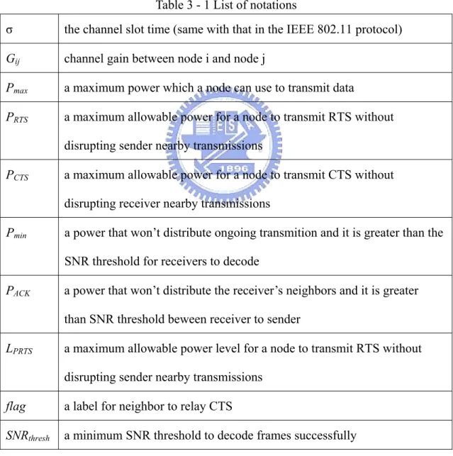
Table 3 - 1 List of notations
σ the channel slot time (same with that in the IEEE 802.11 protocol) Gij channel gain between node i and node j
Pmax a maximum power which a node can use to transmit data
PRTS a maximum allowable power for a node to transmit RTS without
disrupting sender nearby transmissions
PCTS a maximum allowable power for a node to transmit CTS without
disrupting receiver nearby transmissions
Pmin a power that won’t distribute ongoing transmition and it is greater than the
SNR threshold for receivers to decode
PACK a power that won’t distribute the receiver’s neighbors and it is greater
than SNR threshold beween receiver to sender
LPRTS a maximum allowable power level for a node to transmit RTS without
disrupting sender nearby transmissions flag a label for neighbor to relay CTS
SNRthresh a minimum SNR threshold to decode frames successfully
14
power level for senders to receive CTS successfully, and we add the power information Pmin, flag and noise information Nr into CTS frames. We also add the
power information PACK into data frames.
3.3 Neighbor tables
In our protocol, each node maintains a table to keep some information of their neighboring nodes. They construct their neighbor tables, and each table has i entries. Each entries saves one neighbor’s information included “Node ID”, “flag”, “Gain”, “Nr”, “transmission state”, and “Pmin”. “Node ID” is a identifier of neighbors. “flag”
is a label for neighbors to relay CTS. “Gain” is the channel gain between nodes and their neighbors. “Nr” is the noise of neighbors. “transmission state” is a transmission
state of nodes If nodes are transmitting data, we set it to ongoing transmission state. Otherwise, we set it idle state. “Pmin“ is the power for neighbors to transmit data. Each
node updates its neighbor table when it overhears the RTS/CTS packets.
3.4 The proposed protocol
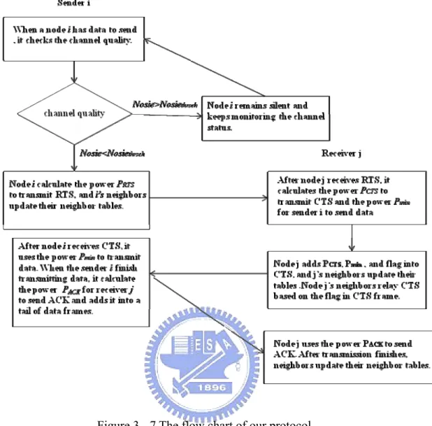
In this section, we introduce how our protocol works. A node i which intends to transmit data to a receiver j checks its Noisethresh,, and then checks its neighbor table.
Node i nearby has m ongoing transmission nodes, and the node j nearby has n ongoing transmission nodes. If the Noisethresh can be met, a node i will calculate a power PRTS to
transmit RTS. Otherwise, node i remains silent and keeps monitoring the channel status. PRTS is a maximum allowable power for a node to transmit RTS without
disrupting its nearby transmissions. We can calculate a power PRTS by equation 1 and
15 α = ) k , i ( d * C ) k , i ( G P P(k) RTS s (k=1,2…..m) (1) In the equation 1, Ps is a free space receiving signal strength of i’s nearby ongoing
transmission node k from the sender i. G( i, k ) is an antenna gain between the sender i and its neighbor k. d( i, k ) is the distance between the sender and its nearby ongoing transmission node k. α is the constant with range 2 to 4. C is a constant depends on the environment.. ) k ( SNR P ) k ( N ) k ( S thresh ) k ( s r n > + (k=1,2…..m) (2)
In the equation 2, Sn(k) is a receiving data signal strength of nearby ongoing
transmission node k. Nr(k) is a noise of nearby ongoing transmission node k.
SNRthresh(k) is a threshold for nearby ongoing transmission node k to decode data
correctly. In the equation 2, we regard it (k) s
P the additional noise to other nearby
transmission nodes k. The additional noise can’t affect every nearby ongoing
transmission node k. Every node k’s SNR must above its threshold. By combining equation 1 and 2, we can get the equation 3.
RTS r thresh n P ) k , i ( G ) k , i ( d * )) k ( N ) k ( SNR ) k ( S ( > α (k=1,2…..m) (3)
The sender i also adds its noise information Nr into RTS. If collisions happen or the
sender i can’t overhear CTS in a period, sender i will retransmission RTS by Pr which we will introduce in the section 3.6. After the intended receiver j receives RTS, it can calculate its channel gain G(i,j) between the sender i. The intended receiver can also
16
calculate a power Pmin for the sender i to transmit data, and the receiver j use PCTS to
transmit CTS message. PCTS must satisfy the following two conditions. First, the
maximum allowable power for a node to transmit CTS can’t disrupt receiver nearby transmissions. We can calculate it by equation 4 and 5.
= α ) k , j ( d * C ) k , j ( G P P(k) CTS r (k=1,2……n) (4) In the equation 4, (k) r
P is a free space receiving signal strength of j’s nearby ongoing transmission node k from the receiver j.
) k ( SNR P ) k ( N ) k ( S thresh ) k ( r r n > + (k=1,2…..n) (5)
In the equation 5, we regard (k)
r
P as the additional noise to other nearby
transmission nodes k. The additional noise can’t affect every nearby ongoing
transmission node k. Every node k’s SNR must above its threshold. By combining equation 4 and 5, we can get the equation 6.
CTS r thresh n P ) k , j ( G ) k , j ( d * C * )) k ( N ) k ( SNR ) k ( S ( > α (k=1,2…..n) (6)
Second, the sender can successfully decode CTS. We can calculate it by equation 7 and 8. α = ) i , j ( d * C ) i , j ( G P P CTS i (7)
17
In the equation 7, P is a free space receiving signal strength of the sender i from the i receiver j. ) i ( SNR P ) i ( N P thresh i r i > + (8)
In the equation 8, the sender i’s receive signal strength is P , and the receive signal i to noise ratio of sender i must above its SNR threshold.
The intended receiver also set one to a fag, and add Pmin, Nr(j), Sn, flag and
SNRthreshold into CTS. Pmin is a power that doesn’t distribute ongoing transmition and it
is greater than SNR threshold for receivers to decode. Pmin also must satisfy the
following two conditions. First, the sender transmitting data can’t disrupt any ongoing transmissions. We can calculate it by equation 9 and equation 10.
= α ) k , i ( d * C ) k , i ( G P P(k) min s (k=1,2…..m) (9) In the equation 9, (k) s
P is a free space receiving signal strength of i’s nearby ongoing transmission node k from the sender i.
) k ( SNR P ) k ( N ) k ( S thresh ) k ( s r n > + (k=1,2…..m) (10)
18 In the equation 10, we regard (k)
s
P as the additional noise to other nearby
transmission nodes k. The additional noise can’t affect every nearby ongoing
transmission node k. Every node k’s SNR must above its threshold. By combining equation 9 and 10, we can get the equation 3.
min r thresh n P ) k , i ( G ) k , i ( d * C * )) k ( N ) k ( SNR ) k ( S ( > α (k=1,2…..m) (11)
Second, Pmin must greater than threshold for the receiver to decode correctly. We can
calculate it by equation12 and 13.
α = ) j , i ( d * C ) j , i ( G P P min j (12)
In the equation 11, Pj is a free space receiving signal strength of the sender i from
the receiver j. ) j ( SNR P ) j ( N P thresh j r j > + (13)
In the equation 13, the receiver j’s receive signal strength is Pj , and the receive signal to noise ratio of receiver j must above its SNR threshold.
19
flag of CTS, if a flag is equal to one, they relay CTS, and set flag zero. After the sender i receives CTS, it transmits data using a instructed power Pmin according to the
information in CTS. When the sender i finish transmitting data, it adds PACK
information into a tail of data frames. PACK must satisfy the following two conditions.
First, a maximum allowable power for a node to transmit ACK cannot disrupt nearby ongoing transmissions. We can calculate it by equation 14 and 15.
α = ) k , j ( d * C ) k , j ( G P P(k) ACK r (k=1,2……n) (14) In the equation 13, (k) r
P is a free space receiving signal strength of j’s nearby ongoing transmission node k from the receiver j.
) k ( SNR P ) k ( N ) k ( S thresh ) k ( r r n > + (k=1,2…..n) (15)
In the equation 15, we regard (k) r
P as the additional noise to the node k. The additional noise can’t affect every nearby ongoing transmission node k. Every node k’s SNR must above its threshold. By combining equation 14 and 15, we can get the equation 16. ACK r thresh n P ) k , j ( G ) k , j ( d * C * )) k ( N ) k ( SNR ) k ( S ( > α (k=1,2…..n) (16)
Second, the sender can successfully decode CTS. We can calculate it by equation 17 and 18.
20 α = ) i , j ( d * C ) i , j ( G P P ACK i (17)
In the equation 7, P is a free space receiving signal strength of the sender i from the i receiver j. ) i ( SNR P ) i ( N P thresh i r i > + (18)
In the equation 17, the sender i’s receive signal strength is P , and the receive signal i to noise ratio of sender i must above its SNR threshold. After the transmission finish, node i and node j’s neighbors update their neighbor tables to change the transmission state from an ongoing transmission state to an idle state.
Here we show the example of our protocol. As shown in Fig. 3-1. ,node A wants to transmit Data to node B. Node A first checks its neighbor table to calculate a power PRTS to transmit a RTS. When node B receives RTS, it computes a channel gain by
receiving RTS signal strngth between a node A and node B, and node B can also calculate a power Pmin for a sender to transmit data, and encapsulates power
information Pmin and noise information into CTS and then return a CTS to node A
with PCTS. When node B’s neighbors overhear a CTS, they update their neighbor table
to change a transmission state from an idle state to an ongoing transmission state and determinate whether to help relaying a CTS. In Fig. 3-2., node A uses Pmin to transmit
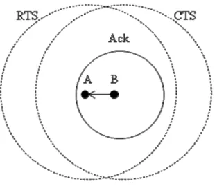
data to node B. In Fig. 3-3., aftert fisnishing transmitting data, node A calculates a power PACK for node B to transmit ACK . The power information PACK added at a
21
A is transmitting data to node B, and node C wants to transmit data to node D. Node C first checks its neighbor table( find node B is receiving data), and it uses a power PRTS to tansmit RTS . Node D uses power PCTS to transmit CTS , and node C uses
Pmin to transmit data. Finally, node D uses PACK to transmit ACK. Fig. 3-6. shows a
basic operation of our protocol. Fig. 3-7. is the flow chart of our protocol.
Figure 3 - 1 Example of our protocol (1)
22
Figure 3 - 3 Example of our protocol (3)
23
Figure 3 - 5 Example of our protocol (5)
24
Figure 3 - 7 The flow chart of our protocol
3.5
Hidden terminals problems
Since a sender may not use maximum powerto transmit control messages, hidden terminal problems may happen as illustrated in Fig. 3-8. In Fig. 3-8., node A is transmitting data to node B, and node C is transmitting data to node D. Since node E does not hear the CTS sent by node D, and node E is in the interference range of node D. If E has packets to transmit to F, it may cause a collision to node C and D.
25
Figure 3 - 8 Hidden terminals problem.
This problem can be solved by neighbors helping relaying CTS messages. When a receiver’s neighbors overhear CTS ,they first calculate their channel gains between a receiver and receiver’s neighbors and calculate the power Pt for forwarding the CTS
message. Pt is the max power which won’t distribute their neighbors. Finally, they can
calculate the number of their neighbor called N that they can relay CTS based on a power Pt and their neighbor tables. If N>0, receiver’s neighbors use Pt to relay CTS.
For example, as shown in Fig. 3-9. and Fig. 3-10. , when node F overhears the CTS messages, it will first calculate the power Pt for relaying CTS. Node E can overhears
CTS by node F relaying CTS. Since node E overhears CTS, it adds node D to its neighbor table. Node E won’t disrupt node D receiving data packets.
This concept is implement by adding a “flag” field in CTS frames. When a node first send CTS, it set a flag to one.When a receiver’s neighbors overhear CTS message, they check the flag field. If the flag is equal to one, they set the flag to zero and relay
26
CTS, and then. On the other hand, they check the flag field equal to zero, they don’t need to relay CTS. By the way, we put the flag in the RESV(a unused field in 802.11 header)
Figure 3 - 9 Example of nodes relay CTS in our protocol (1)
27
3.6 Contention resolution
When nodes want to transmit data, they have a probability Pr to send RTS. Pr is propotion to maximum allowable power (LPRTS).
) 2 1 ( * A L = Pr PRTS r (19) LPRTS is the maximum allowable power for a node to transmit RTS without disrupting
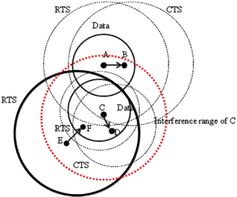
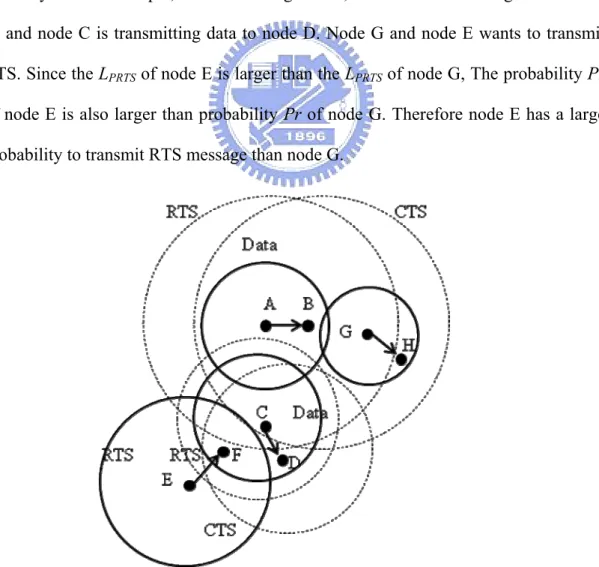
nearby transmissions and A is a constant to optimize the probability Pr. r is the number of retransmission value, and its initial value is zero. When retransmission times increase, Pr decrease. When collisions happen, nodes retransmit RTS with probality Pr. For example, as shown in Fig. 3-11. , node A is transmitting data to node B, and node C is transmitting data to node D. Node G and node E wants to transmit RTS. Since the LPRTS of node E is larger than the LPRTS of node G, The probability Pr
of node E is also larger than probability Pr of node G. Therefore node E has a large probability to transmit RTS message than node G.
28
Now we define the probability Pc to avoid collisons from relaying CTS messages. Probability Pc direct proportion to the number of neighbors that can are with the transmission range of power Pt .
) 2 1 ( * B N = Pc r (20)
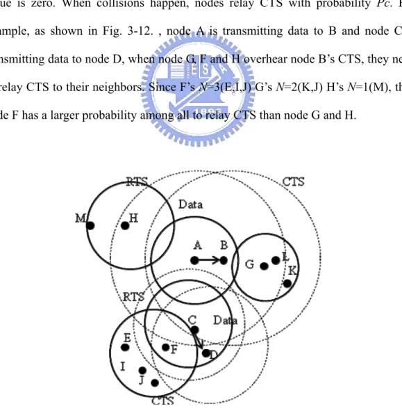
where N is the number of neighbor that can reach by power Pt, and B is a constant to optimize the probability Pc. r is the number of retransmission times, and its initial value is zero. When collisions happen, nodes relay CTS with probability Pc. For example, as shown in Fig. 3-12. , node A is transmitting data to B and node C is transmitting data to node D, when node G, F and H overhear node B’s CTS, they need to relay CTS to their neighbors. Since F’s N=3(E,I,J) G’s N=2(K,J) H’s N=1(M), thus node F has a larger probability among all to relay CTS than node G and H.
29
3.7 Performance analysis
In this section, we introduce the model analysis with our protocol. We will describe the preliminaries of our protocol, and then we use the preliminaries to calculate the throughputs of our protocol.
A. Preliminaries
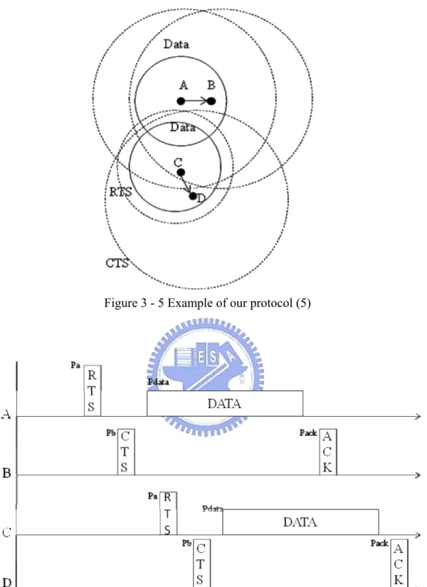
We assume that RTS, CTS, DATA, and ACK packets are with fixed lengths of LRTS , LCTS, Ldata and LACK. R is the data rate. Tr, Tc, Tdata, and TACK are transmission
times of RTS, CTS, DATA, and ACK packets. We can calculate them by equation (21), (22), (23), and (24). R L T RTS r = (21) R L T CTS c = (22) R L T data data = (23) R L T ACK ACK = (24)
Let τ be the probability that a node will transmit data in a time period
τ=α*β (25)
α is a probability of the packet arrival probability, and we assume the process follow a poisson distribution. β is a probability that a node will be selected to transmit data, and it depends on the simulation environment.
30 T l e ! l ) T ( α = λ λ ( l = 0,1,2……) (26) In the equation 26, where λ is the frame arrival rate and T is the expected duration of a successful transmission, a collision, and slots being idle.
Let Pi be a probability that a sender has no frame to send. Pi can be expressed as the
equation 27. In the equation 27, τ is a probability that a node will transmit data in a time period. 1-τ is a probability that a sender has no frame to send.
τ -1 =
Pi (27)
Let Pc be a probability that a transmitted frame experiences a collision. Pc can be
expressed as
Pc = τ ( 1 - ( 1 - τ )Nc – Nr -1 ) (28) where Nc is a number of the nodes in the collision area, and Nr is the number of nodes
that the receiver’s neighbor can relay.
Nc = π ( Rmax - Rmin )2 ρ (29)
Nr = π ( 1.5Rmin - Rmin )2 ρ (30)
ρ is a the density distribution of nodes
Rmin is the distance between a sender and a receiver.
Rmax is the max distance that a sender can send a message
31
the number of nodes that the receiver’s neighbor can relay, 1-(1 - τ )Nc-Nr-1 means the probability of all nodes in the collision area will at least one node try to transmit data. τ(1− (1 − τ )Nc-1) means the probability that a node will cause collisions.
Let Pb be a probability that a sender sense the channel busy, and Pb can be
expressed as
Pb = τ ( 1 - ( 1 - τ )Nb ) (31)
where Nb is a number of the nodes in the transmission area.
Nb = π ( Rmin )2ρ (32)
In the equation 31, Since Nb is a number of the nodes in the busy area, 1- (1 - τ )Nb-1
means the probability of all nodes in the busy area will at least one node try to transmit data. τ (1 - (1 - τ )Nb-1) means the probability that a node will cause collisions.
Let Pt be a probability of a sender’s successful transmission. Pt can be expressed as
the equation 33. ) _ _ _ _ _ _
(successful send packets have packets to send
P Pt = ∩ (33) ) _ _ ( ) _ _ ( ) _ _ ( ) _ _ _ ( packets send fail P packets send successful P packets send successful P send to packets have P + × =
32 Nb Nc Nb Nc Nb Nc τ) -(1 τ) -(1 τ) -(1 -(1 τ) -(1 -(1 τ) -(1 -(1 τ) -(1 -(1 τ + + = B. Performance analysis
The throughput S for each transmitter is calculated as the amount of successful Transmission (bits) per unit time slot (second). S can be expressed as
avg t T ] P [ E P S =
(34)
where E[P] is the average packet length and Tavg is the average time. Tavg can be
expressed as
Tavg = Pi Ti + PbTb + PcTc + PtTt (35)
where Ti is the duration of an idle slot. Tb is an average time that a sender is sensed
busy because of a successful transmission. Tc is an average time the sender is sensed
busy by the stations during a collision. Tt is an average time a sender is successfully
transmission. Ti, Tb, Tc, and Tt can be expressed as
Ti = σ (36)
Tc = DIFS + Tr + ω (37)
Tb= DIFS + (PHYhdr + MAChdr ) / R + (Tr + Tc + TACK + Tdata ) +4ω+3 * SIFS (38)
Tt= (PHYhdr+MAChdr )/R + DIFS+ 4*ω + 3*SIFS +( Tr + Tc + TACK + Tdata ) (39)
where σ is a duration of an empty slot time, and ω is a propagation delay time. Fig.3-13 shows a time diagram of packet transmission time.
33
34
Chpater 4 Performance Evaluation
In this chapter, we evaluate the performance of our protocol and compare it with POWMAC and the IEEE 802.11 scheme. We use NS2 (version 2.33) [11] to evaluate the proposed protocol. We compare our protocol with POWMAC because the latter one is also a transmission power control MAC protocol based on a single channel, single transceiver design. In this chapter, we will introduce the environment setting and the simulation result will be shown.
4.1 Environment setting
In this section, we will show the parameters used in our protocol. Some parameters of IEEE 802.11 is shown in table 4-1.
Table 4 - 1 Simulation and analysis parameters
Simulation times 60 second
A 0.28
B 8
Data packet size 2 KB
Data rate 1 Mbps
SINR threshold 6 dB
Max Transmission range 250 meters
Carrier sensing threshold 3.44283e-09 joule
Propagation Model Two-Ray Ground
CWMin 31 CWMax 1023
35
Preamble Length 144
PLCP Header Length 48
PLCP Data Rate 1.0e6
Short Retry Limit 7
Long Retry Limit 4
We consider four scenarios according to different topologies and mobility constrains. In the first scenario, we first assume a linear topology and a node will move toward with one node. In the second scenario, we construct 25 nodes separate in a 500*500 square area. In the third scenario, nodes in second scenario will random move toward any direction. In the fourth scenario, we set particular position of six nodes to see the performance of relaying CTS. We compare our protocol in relaying CTS and without relaying CTS method.
4.2 Scenario one
We first simulate a linear topology for the purpose of highlighting the advantages and operational details of our protocol. The distances between the terminals are also shown in the Figure. 4-1. Terminal A is first transmitting to node B, and then node C is transmitting to node D. In this scenerio, node B starts moving to node C at a speed of 1.5 m/s.
36
Figure 4 - 1 A Line topology for scenario one
Fig. 4-2 depicts the throughput of the network. We can see the performance of our protocol is better than POWMAC and IEEE 802.11 MAC. In POWMAC, when nodes want to send data, they need to wait the channel clear and the AW window times. The nodes also need to wait the AW time counter ended even the network is not very crowded. In IEEE 802.11 MAC, nodes can send data only when the channel is clear. In the first scenario, only one transmission can proceed at a time since all terminals are within the carrier-sense range of each other. However, according to our protocol, in first 10s, the two transmissions A->B and C->D can proceed simultaneously. For the next 40s, when node C gets closer to node B, noises increase between node B and C, and throughputs decrease. After 50s, the interferences become larger than the threshold, node C will not try to transmit data. Therefore, only node A exchanges RTS/CTS with node B, node C can’t transmit to node D.
37
4.3 Scenario two
We now study the performance under more realistic network topologies. We distribute 25 terminals in a 500m*500m square area. The square is split into 25 smaller square areas, one for each terminal. The location of a terminal within the small square is selected randomly. For each sender, the destination terminal is selected randomly from the one-hop neighbors. We randomly pick ten terminals to send data.
Figure 4 - 3 The topology of scenario two
The performance is shown in Fig. 4-4. It is easy to obvious that the performance of our protocol is better than POWMAC and IEEE 802.11 protocol in different data rates. In IEEE 802.11 only few pairs can transmit simultaneously. In the simulation, we observe than only 3 nodes can transmit data simultaneously in 802.11. In POWMAC, 5 nodes can transmit data simultaneously. In our protocol, 7 nodes can transmit data simultaneously. Since in IEEE 802.11, nodes overhearing RTS/CTS message, they
38
will set NAV and they can’t send any data. In POWMAC, it needs to use the AW windows to synchronize the transmission. It wastes the AW windows time and data transmission need to synchronize. It can’t make sure that all data is sent to the destination on time. Since POWMAC needs to transmit extra packet “DTS” for synchronization, a extra overhead also reduce throughputs. In our protocol, we can let multiple transmissions exist without synchronization, and our protocol doesn’t need to waste the AW windows time. Although our protocol adjust the power of control messages and relay CTS messages, the hidden terminal problem still can’t completely be avoided. The performance of our protocol can’t complete match with the analysis performance.
Figure 4 - 4 Throughputs in the scenario two
4.4 Scenario three
In scenario three, we add the mobility to nodes in the second scenario. The terminals are randomly selected the direction and their speeds are 0.3m/s. The performance is shown in Fig. 4-5. The performance of our protocol is still better than
39
POWMAC and IEEE 802.11. We adjust the proper power to send data. If nodes move, SNR of a channel will decrease, and we will increase the power until it reaches its upper bounded. The upper bounded power can’t disturb ongoing pairs. Similarly, since we can’t complete avoid hidden terminals problem, we can’t complete match with the analysis performance.
In Fig. 4-6., we set nodes with different speeds between 0.3m/s to 0.7m/s. We can observe that when speeds increase, the throughput of our protocol will decrease. At the beginning, 7 nodes can transmit data simultaneously in our protocol, and 5 nodes can transmit data simultaneously. Throughput of our protocol is 25% up to POWMAC. As time goes by, the distance between senders and receivers increase. Since senders need to use more power to transmit data, number of nodes which can transmit data simultaneously decreases, and throughputs also decrease.
Fig. 4-7 shows energy consumption in different scenarios. We can observe that energy consumption of our protocol is 18% low to IEEE 802.11 and 15% up to POWMAC. Since in IEEE 802.11, nodes always use a maximum power to send data, nodes wastes a lot of power in data transmission. Our protocol needs to relay CTS to avoid hidden terminal problems, power consumptions are more than POWMAC. Although our protocol wastes more power than POWMAC, throughputs in our protocol is better than POWMAC. In Fig. 4-8., we can observe that power consumptions per packet. Power consumption per packet in our protocol is 50% low to IEEE 802.11 and 14% low to POWMAC.
In Fig. 4-9, we compare our protocol with relay CTS and without relay CTS method. We observe that when nodes in speed of 3 m/s, throughputs of relay CTS
40
method is higher than without relay method by upper to 15%. When the speed increases, relay CTS method throughputs gradually decrease. When nodes in the speed of 0.7 m/s, throughputs of relay CTS method is close to without relay CTS method. Since nodes moving fast, the relaying CTS method can’t completely relay CTS information to the hidden terminals.
In Fig.4-10 shows energy consumption in different scenarios. We can observe that energy consumption of without-relay-CTS protocol is 17% low to with-relay-CTS protocol. Since nodes may waste some power relay CTS, the energy consumption is more than nodes without relay CTS. In Fig. 4-11, we observe that with-relay-CTS method consumes less energy per Kbps than without-relay-CTS method. Although with-relay-CTS method need to waste some energy to relay CTS, it throughputs is better than without-relay-CTS method. The energy consumption per Kbps is also less than without relay CTS method.
41
Figure 4 - 6 Throughputs of different speeds
42
Figure 4 - 8 Energy consumption per packet in different scenarios
Figure 4 - 9 Throughputs of relay CTS method and without relay CTS method in different speeds
43
Figure 4 - 10 Energy consumption in different scenario
Figure 4 - 11 Energy consumption per Kbps in different scenario
4.5 Scenario four
In the section 3.4, we relay the CTS message to avoid the hidden terminals problems. In order to testing the method of relaying CTS message, we build the topology in the scenario four. The distances between terminals are also shown in the figure. 4-12. We set three flows in the scenario four, A->B, D->C and E->F.
44
Figure 4 - 12 The topology to show the effect of relaying CTS
The Fig. 4-13 shows the performance of relay CTS and without CTS. In Fig. 4-13, we observe node E doesn’t know the ongoing pair D->C in without relay CTS protocol. Node E will use a maximum power to send control messages, so the ongoing pair D->C will be disturbed. Only A->B pair can successful transmission data. In relay-CTS protocol, node F will relay CTS to node E. Node E can adjust the transmission power. Hence A->B, D->C and E->F can transmit simultaneously.
45
Chpater 5 Conclusion and Future Work
Since in IEEE 802.11 MAC protocol, when nodes want to transmit data, they need to wait channels clear, and expose problems will happen. However, in IEEE 802.11 physical layer (PHY), nodes can correct decode packets when signal to noise ratio (SNR) reaches a threshold. We combine the packets decode threshold in PHY and sensing channel clear data transmission in MAC layer. We modify IEEE 802.11 MAC protocol based on SNR threshold in PHY layer.In this essay, we propose a new adaptive transmission power control MAC protocol, which can significantly improve the network throughputs using a single channel and single transceiver environment. Dissimilar with IEEE 802.11, our protocol doesn’t need to wait the channel clear. We adjust the transmission power of control and data packets based on SNR information. When the channel quality is good enough, nodes will start to transmit data. Dissimilar with POWMAC, we adjust of transmission power of control packets instead of data synchronization. The reason is that data synchronization will increase packets delay time, and nodes need to wait some times to transmit data. Since our protocol doesn’t use extra packets, the packets overhead are less than POWMAC. We also consider hidden terminals problems by relaying CTS to receivers’ neighbors. In order to verify our protocol, we analyze throughputs of our protocol and we use ns2 to run simulations.
In simulations, we compare throughputs and power consumption of our protocol, POWMAC, and IEEE 802.11 in four scenarios of different topologies. The simulation has shown that throughput in our protocol is better than POWMAC and IEEE 802.11
46
protocol, and the power consumption in our protocol is more than POWMAC but less than IEEE 802.11.
Some limitations are still on our protocol. First, if nodes speed increase fast, the neighbor table cannot update immediately. Second, since we relay CTS, the power consumptions increase. We will discuss these issues in the future.
47
References
[1] IEEE 802.11 working group. Wireless LAN medium access control (MAC) and physical layer (PHY) specifications.(1999)
[2] IEEE 802.11 working group. Wireless LAN medium access control(MAC) and physical layer (PHY) specifications: high-speed physical layer in the 5GHz Band, (1999)
[3] IEEE 802.11 working group. Wireless LAN medium access control (MAC) and physical layer (PHY) specifications: higher-speed physical layer extension in the 2.4GHz Band, (1999).
[4] Jeffrey P. Monks, Vaduvur Bharghavan, and Wen-mei W. Hwu, “A Power Controlled Multiple Access Protocol for Wireless Packet Networks,” in Proc. IEEE International Conference on Computer Communications (INFOCOM’01), San Francisco, California, USA, Mar. 2001
[5]A. Muqattash and M. Krunz, “Power controlled dual channel (PCDC) medium
access protocol for wireless ad hoc networks,” in Proc. IEEE International
Conference on Computer Communications (INFOCOM’03), San Francisco, California, USA, Mar. 2003.
[6] A. Muqattash and M. Krunz, “POWMAC: a single-channel power-control protocol for throughput enhancement in wireless ad hoc networks,” IEEE J. Select. Areas Communications , vol. 23, no. 5, pp. 1067–1084, May 2005.
[7] Bassel Alawieh, Chadi Assi and Wessam Ajib, “A Power Control Scheme for
Directional MAC Protocols in MANET,” in Proc. IEEE Wireless Communications
and Networking Conference, Hong Kong, March 2007.
[8] Swades De, Komlan Egoh and Gaurav Dosi, “receiver initiated power control multi-access protocol in wireless ad hoc networks,” in Proc. IEEE Sarnoff Symposium,
48 New Jersey, USA , May 2007.
[9] Kuei-Ping Shih, Chau-Chieh Chang and Yen-Da Chen, “A Fragmentation-based Data Collision Free MAC Protocol with Power Control for Wireless Ad Hoc Networks,” in Proc. I IEEE Wireless Communications and Networking Conference, Las Vegas, USA, April 2008.
[10] Minghao Cui and Violet R. Syrotiuk, “Fair Variable Transmission Power
Control” in Proc. IEEE Global Telecommunications Conference, Washington, DC,
USA, November 2007.
[11] NS-2 simulator, http://www.isi.edu/nsnam/ns/
[12] C. Ware, J. Chicharo, and T. Wysocki, “Simulation of capture behavior in IEEE 802.11 radio modems,” in Proc. IEEE Veh. Technol. Conf., vol.3, Fall 2001, pp. 1393– 1397.
[13] R. Wattenhofer, L. Li, P. Bahl, and Y.-M. Wang, “Distributed topology control for power efficient operation in multihop wireless ad hoc networks,” in Proc. IEEE INFOCOM Conf., 2001, pp. 1388–1397.
[14] S.-L. Wu, Y.-C. Tseng, and J.-P. Sheu, “Intelligent medium access for mobile ad hoc networks with busy tones and power control,” IEEE J. Sel. Areas Commun., vol. 18, no. 9, pp. 1647–1657, Sep. 2000.
[15] K. Xu, M. Gerla, and S. Bae, “How effective is the IEEE 802.11 RTS/CTS handshake in ad hoc networks,” in Proc. IEEE GLOBECOM
Conf., vol. 1, Nov. 2002, pp. 72–76.
[16] C.-H. Yeh, “ ROAD: A variable-radiusMAC protocol for ad hoc wireless networks,” in Proc. IEEE Veh. Technol. Conf., vol. 1, 2002, pp. 399–403.
[17] H. Zhou, C.-H. Yeh, and H. Mouftah, “ A solution for multiple access in variable-radius mobile ad hoc networks,” in Proc.IEEE Int. Conf. Commun., Circuits, Syst. , vol. 1, 2002, pp. 150–154.