基於類神經網路之蛋白質金屬鍵結胺基酸預測

全文

(1)國立交通大學電機與控制工程學系碩士論文. 基於類神經網路之蛋白質金屬鍵結胺基酸預測. Protein Metal-Binding Residue Prediction Based on Neural Networks 研究生：楊志賢指導教授：王啟旭博士林進燈博士楊裕雄博士中華民國九十三年六月.

(2) 基於類神經網路之蛋白質金屬鍵結胺基酸預測 Protein Metal-Binding Residue Prediction Based on Neural Networks. 研究生：楊志賢. Student：Chih-Hsien Yang. 指導教授：王啟旭博士. Advisor：Dr. Chi-Hsu Wang. 林進燈博士. Co-Advisor：Dr. Chin-Teng Lin. 楊裕雄博士. Co-Advisor：Dr. Yuh-Shyong Yang 國立交通大學. 電機與控制工程學系碩士論文. A Thesis Submitted to Department of Electrical and Control Engineering College of Engineering and Computer Science National Chiao Tung University in Partial Fulfillment of the Requirements for the Degree of Master in Electrical and Control Engineering June 2004 Hsinchu, Taiwan, Republic of China. 中華民國九十三年六月.

(3) 基於類神經網路之蛋白質金屬鍵結胺基酸預測學生：楊志賢. 指導教授：王啟旭博士共同指導教授：林進燈博士共同指導教授：楊裕雄博士. 國立交通大學電機與控制工程研究所. 摘要傳統上，結構生物學家利用物理實驗的方式去了解金屬蛋白 (與金屬產生鍵結的蛋白質) 的特性，並藉由其立體結構與實驗上的觀察去推論酵素產生功能的原因及其反應機制。然而，大多數的蛋白質都已知其一級結構 (胺基酸序列組成) ，立體結構資訊卻不如序列資訊來的普遍。再者，目前由序列資訊預測蛋白質立體結構的技術，也仍尚未達到絕對可靠的階段。. 因此，本論文中提出，純粹以蛋白質序列的資訊，使用類神經網路為主要核心的預測器，搭配滑動框架式特徵擷取以及生物化學式特徵編碼的技術，對蛋白質金屬鍵結胺基酸進行預測。針對生命系統中的四種主要金屬 (鈣、鉀、鎂與鈉) 鍵結蛋白質中，在五等份的交叉驗證中，均可達到九成以上的鍵結偵測敏感度且兼具極佳的準確度。. 關鍵字：生物資訊學，類神經網路，金屬蛋白，酵素。. i.

(4) Protein Metal-Binding Residue Prediction Based on Neural Networks Student: Chih-Hsien Yang. Advisor: Dr. Chi-Hsu Wang Co-Advisor: Dr. Chin-Teng Lin Co-Advisor: Dr. Yuh-Shyong Yang. Department of Electrical and Control Engineering National Chiao Tung University Abstract Traditionally, structural biologists used to investigate properties of metalloproteins (proteins which bind with metal ions) by physical means and interpret the function formation and reaction mechanism of enzyme by their structures and observation from experiments in vitro. Most of proteins have primary structures (amino acid sequence information) only; however, the 3-dimension structures are not always available. Moreover, the prediction from protein sequence to structure is still not completely reliable so far.. Consequently, a direct analysis method is proposed to predict protein metal-binding amino acid residues only from its sequence information by neural network with sliding window-based feature extraction and biochemical feature encoding techniques in this thesis. In four major bulk elements (Calcium, Potassium, Magnesium, and Sodium) in life system, the metal-binding residues are identified with a binding sensitivity > 90% and nearly 100% accuracy under five fold cross validation.. KEYWORD：Bioinformatics, Neural Networks, Metalloprotein, Enzyme. ii.

(5) 致. 謝. 獻給所有陪我一路走來的人。. iii.

(6) Acknowledgements To these who go along with me through this way.. iv.

(7) Contents Chinese Abstract ................................................................................................ i English Abstract ................................................................................................ ii Chinese Acknowledgements ............................................................................ iii English Acknowledgements............................................................................. iv Contents ............................................................................................................. v List of Tables..................................................................................................... vi List of Figures.................................................................................................. vii Chapter 1 Introduction.................................................................................. 1 1.1 1.2 1.3. Introduction to Bioinformatics.......................................................................1 Metalloprotein and Motivation ......................................................................3 Thesis Organization .......................................................................................8. Chapter 2 Biological Resource ...................................................................... 9 2.1 2.2 2.3. Integration of Web Biological Databases.......................................................9 Metal Binding Model and Database Design ................................................15 Biological Data Processing and Sampling...................................................18. Chapter 3 Machine Learning Scheme........................................................ 24 3.1 3.2. Neural Networks ..........................................................................................24 Feature Encoding .........................................................................................25. Chapter 4 Results and Conclusion ............................................................. 28 4.1 4.2 4.3. Performance Measures.................................................................................29 Experiments on One-hot Coding Method ....................................................30 Comparison between Different Feature sets ................................................34. References ........................................................................................................ 38 Appendix .......................................................................................................... 40 [A] [B] [C]. MySQL, Apache and PHP ...........................................................................40 PDB File Format ..........................................................................................40 Clustalw and Blast .......................................................................................43. v.

(8) List of Tables TABLE 1.1.A GROWTH IN GENBANK (LEFT) AND PROTEIN DATA BANK (RIGHT) .......................................2 TABLE 1.2.A TABULAR COMPARISON OF ENZYME PERCENTAGE IN DIFFERENT SETS ..................................5 TABLE 1.2.B MAJOR ENZYME CLASSES AND FUNCTIONS ...........................................................................6 TABLE 2.1.A PROTEIN TABLE IN MDB ....................................................................................................10 TABLE 2.1.B SITE TABLE IN MDB........................................................................................................... 11 TABLE 2.1.C LIGAND TABLE IN MDB ..................................................................................................... 11 TABLE 2.1.D RECORD ORGANIZATION IN LEVEL (1) PROTEIN ...............................................................14 TABLE 2.1.E RECORD ORGANIZATION IN LEVEL (2) CHAIN ...................................................................14 TABLE 2.1.F RECORD ORGANIZATION IN LEVEL (3) HET-GROUPS ..........................................................15 TABLE 2.3.A NUMBER OF SITE IN MDB RELEASED FILES ........................................................................19 TABLE 2.3.B NUMBER OF CHAINS IN PROTEIN SET AND ENZYME SET AFTER CROSS QUERYING ................21 TABLE 2.3.C PROTEIN SET SIZE UNDER DIFFERENT SEQUENCE IDENTITY THRESHOLD .............................22 TABLE 2.3.D ENZYME SET SIZE UNDER DIFFERENT SEQUENCE IDENTITY THRESHOLD .............................23 TABLE 3.2.A ONE-HOT CODING TABLE FOR 20 AMINO ACIDS ...................................................................25 TABLE 3.2.B DEFINITIONS OF FIVE BIOLOGICAL FEATURE SETS ...............................................................26 TABLE 3.2.C VALUES OF FIVE BIOLOGICAL FEATURE SETS .......................................................................26 TABLE 4.1 DETAILED PERFORMANCE MEASURES AND COMPARISON .......................................................29 TABLE 4.2.A Q-OBSERVED OF 31 ELEMENTS IN ENZYME SET W.R.T. DIFFERENT WINDOW SIZE.................30 TABLE 4.3.A COMPARISON OF ONE-HOT CODING AND 5 BIOLOGICAL SETS IN BULK ELEMENTS ...............34 TABLE B.1 PDB FILE FORMAT OVERVIEW PART 1 ....................................................................................41 TABLE B.2 PDB FILE FORMAT OVERVIEW PART 2 ....................................................................................41 TABLE B.3 PDB FILE FORMAT OVERVIEW PART 3 ....................................................................................40 TABLE B.4 SECTIONS IN PDB FILE ..........................................................................................................42 TABLE B.5 RECORD TYPES IN PDB FILE..................................................................................................42 TABLE C.1 IMPORTANT COMMANDS IN BLAST PACKAGE .......................................................................43 TABLE C.2 IMPORTANT COMMANDS IN CLUSTALW PACKAGE ..................................................................43 TABLE C.3 FULL COMMANDS OF CLUSTALW PACKAGE ............................................................................44. vi.

(9) List of Figures FIG 1.2.B METAL-BINDING PROTEINS IN 19771 PROTEINS .........................................................................4 FIG 1.2.C ENZYMES IN 7250 METAL BINDING PROTEINS ............................................................................4 FIG 1.2.D HISTOGRAM OF ENZYME PERCENTAGE COMPARISON .................................................................5 FIG 1.2.E 3D METAL-BINDING STRUCTURE OF CARBONIC ANHYDRASE II ..................................................8 FIG 2.1.A METAL-LIGAND DIAGRAM IN METAL-BINDING PROTEIN ..........................................................10 FIG 2.1.B FORMAT OF LIGAND FILE IN MDB PACKAGE ............................................................................ 11 FIG 2.1.C AN EXAMPLE OF RELEASED TEXT FILE IN PDBFINDER .............................................................15 FIG 2.2.A DSD SCHEMATIC OF PDBFINDER ............................................................................................16 FIG 2.2.B DSD SCHEMATIC OF MDB.......................................................................................................16 FIG 2.2.C METAL-BINDING PROTEIN DATA HIERARCHY ...........................................................................17 FIG 2.2.D ENTITY RELATIONSHIP DIAGRAM OF PDBFINDER AND MDB ..................................................18 FIG 2.3.A DATA PROCESSING PIPELINE.....................................................................................................19 FIG 2.3.B LIFE ELEMENTS IN PERIODIC TABLE .........................................................................................20 FIG 3.1.A SIMPLE FULL CONNECTION NEURAL NETWORKS .......................................................................24 FIG 3.2.C FEATURE EXTRACTION, LEARNING SCHEME AND SLIDING WINDOW .........................................27 FIG 4.A FIVE FOLD CROSS VALIDATION ....................................................................................................28 FIG 4.2.A Q-OBSERVED OF 4 BULK ELEMENTS BY ONE-HOT CODING .......................................................31 FIG 4.2.B Q-OBSERVED OF 11 TRACE ELEMENTS BY ONE-HOT CODING ....................................................31 FIG 4.2.C Q-OBSERVED VERSUS TRAINING EPOCH OF BULK ELEMENTS ...................................................32 FIG 4.3.B Q-OBSERVED COMPARISON BETWEEN DIFFERENT FEATURE SETS AND BULK ELEMENTS ...........36 FIG 4.3.C Q-PREDICTED COMPARISON BETWEEN DIFFERENT FEATURE SETS AND BULK ELEMENTS ..........36 FIG 4.3.D Q-PREDICTED VERSUS TRAINING EPOCH BETWEEN DIFFERENT FEATURE SETS .........................37. vii.

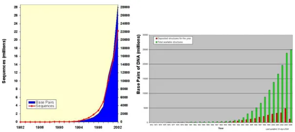
(10) Chapter 1 Introduction 1.1 Introduction to Bioinformatics1 With rapid growth in computer and information science in recent years, most things in daily life have changed the way they were including biology － the study of living things. From last several decades, biologists have collected and accumulated data from interaction of spices and populations, the function of tissues and cells within an individual organism, and even the structure and function of molecules (such as protein, DNA, RNA, etc.) inside or outside the cell. Sophisticated laboratory technology today helps biologists collect data faster, but it can’t speed up the interpretation of these massive and divergent biological data.. For instance, we have huge volume of human DNA sequences after Human Genome Project (HGP)2, but how do we know which parts of DNA sequence can control which kinds of chemical processes or reactions in human body (Gene annotation or labeling)? We have many outstanding structural biologists spent great effort on determining protein structures by Nuclear Magnetic Resonance (NMR) or X-ray crystallography, and figuring out the structure of some proteins, but how do we determine the structure and function of other proteins and even a whole new protein (protein structure prediction and function analysis)? Table 1.1.a show the exponential data growth in GenBank3 and Protein Data Bank4 respectively. Consequently, it is necessary for biologists to use current computational and 1. 2. 3. 4. Use of computers in biological research, such as the use computerized databases for genomes, proteins, etc. It is an international research effort to identify sequence and map all genes in human DNA. http://www.ornl.gov/sci/techresources/Human_Genome/home.shtml GenBank is the NIH (National Institutes of Health, http://www.nih.gov/) genetic sequence database, an annotated collection of all publicly available DNA sequences. http://www.ncbi.nlm.nih.gov/Genbank/genbankstats.html It is a single worldwide repository for the processing and distribution of 3-D biological macro-molecular structure data. http://www.rcsb.org/pdb/ 1.

(11) internet technologies to help them store, share and analyze their biological data on computer or world-wide-web instead of their hands and eyes so as to yield “high throughput” biology, and accelerate the discovery in life science and development of biomedical products, such as drug, and therapy for cancers or other currently unsolvable diseases.. But unfortunately, bioinformatics have become a buzzword with the hype about mapping the human genome. All of these wonderful dreams should be based on every small pieces of understanding about the whole organism from top to toe, and not based on the exaggeration of newspaper or people’s short passion and day dream.. Table 1.1.a Growth in GenBank (left) and Protein Data Bank (right). 2.

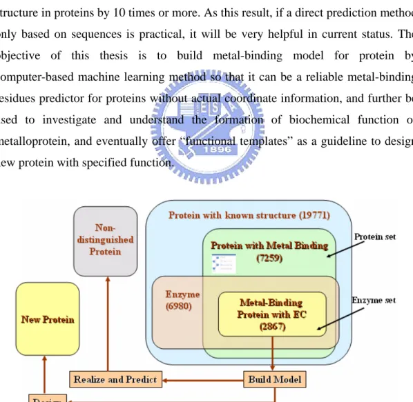
(12) 1.2 Metalloprotein and Motivation Metalloproteins are proteins capable of binding one or more metal ions, which are required for their biological function or for regulation of their activities or even for structure purposes. It is very interesting and amazing that more than one-quarter of the elements in periodic table are required for life (as shown in Figure 2.3.b) , and most of them are metal ions. According to 5PIR, the release 78.03 contains 283,336 entries in November 24, 2003. In contrast, in Protein Data Bank there are 24,358 structures are available in February 17, 2004. Transparently, the sequence material is greatly richer than the structure in proteins by 10 times or more. As this result, if a direct prediction method only based on sequences is practical, it will be very helpful in current status. The objective of this thesis is to build metal-binding model for protein by computer-based machine learning method so that it can be a reliable metal-binding residues predictor for proteins without actual coordinate information, and further be used to investigate and understand the formation of biochemical function of metalloprotein, and eventually offer “functional templates” as a guideline to design new protein with specified function.. Figure 1.2.a Overview of data resource and working map 5. Protein Information Resource, an integrated public resource of protein informatics to support genomic and proteomic research and scientific discovery. http://pir.georgetown.edu/ 3.

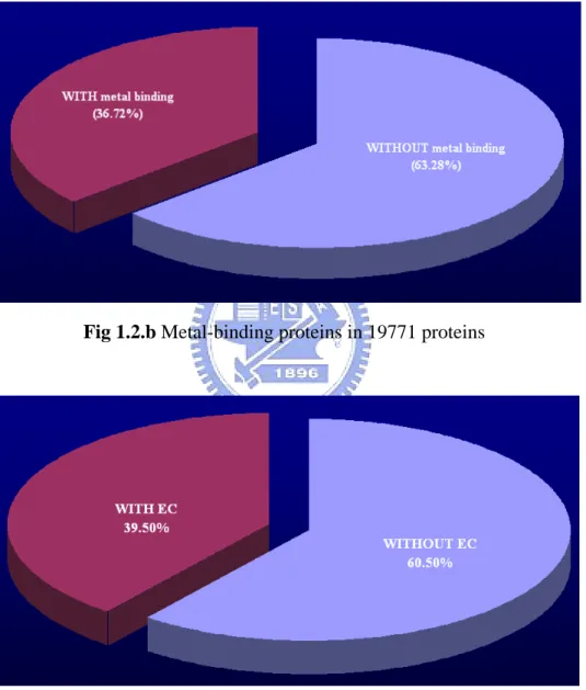
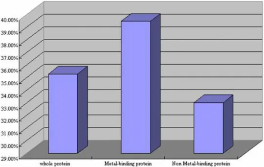
(13) In this thesis, two major data sets (protein set and enzyme set, as shown in Figure 1.2.a) are extracted from 19771 protein structures in PDB and all experiments are based on enzyme set. There are 7529 protein molecules with metal binding and 6890 protein molecules with EC number6. Besides, there are over one-third (36.72%) proteins containing metal ions in 19771 protein structures and nearly 40% of them are enzymes (Figure 1.2.b and 1.2.c).. Fig 1.2.b Metal-binding proteins in 19771 proteins. Fig 1.2.c Enzymes in 7250 metal binding proteins. In Table 1.2.a and Figure 1.2.d show the comparison of enzyme percentage. 6. Enzyme Commission number, a nomenclature for enzymes, developed by The International Union of Biochemistry and Molecular Biology, is described by a sequence of four numbers, preceded by “EC” in the form of “EC X.X.X.X.” 4.

(14) between metal-binding protein set, non metal-binding protein set and entire protein set, a protein with metal binding is more likely to be an enzyme.. Table 1.2.a Tabular comparison of enzyme percentage in different sets. Fig 1.2.d Histogram of enzyme percentage comparison. An enzyme, in biology, is a special protein molecule whose function is to facilitate or accelerate most chemical reactions in cells. Many chemical reactions occur within biological cells, but most of them happen too slowly without catalysts in vitro (test tube) to be biologically relevant.. By common convention, an enzyme’s name is a description of what is does, with the word ending “-ase” added, such as alcohol dehydrogenase and DNA polymerase. The International Union of Biochemistry and Molecular Biology has developed a nomenclature for enzymes, the EC numbers; each enzyme is described by a sequence of four numbers, preceded by “EC” in the form of “EC X.X.X.X.” The 5.

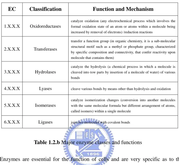
(15) first number broadly classified the enzyme based on its mechanism as below：. EC. Classification. 1.X.X.X. Oxidoreductases. Function and Mechanism catalyze oxidation (any electrochemical process which involves the formal oxidation state of an atom or atoms within a molecule being increased by removal of electrons) /reduction reactions transfer a function group (in organic chemistry, it is a sub-molecular. 2.X.X.X. Transferases. structural motif such as a methyl or phosphate group, characterized by specific composition and connectivity, that confer reactivity upon molecule that contains them) catalyze the hydrolysis (a chemical process in which a molecule is. 3.X.X.X. Hydrolases. cleaved into tow parts by insertion of a molecule of water) of various bonds. 4.X.X.X. Lyases. 5.X.X.X. Isomerases. cleave various bonds by means other than hydrolysis and oxidation catalyze isomerization changes (conversion into another molecules with the same molecular formula but different arrangement of atoms, called isomers) within a single molecule. 6.X.X.X. Ligases. join two molecules with covalent bonds. Table 1.2.b Major enzyme classes and functions Enzymes are essential for the function of cells and are very specific as to the reactions they catalyze and the chemicals (substrates) that involved in the reactions. Substrates fit their enzymes like a key fits its lock. Many enzymes are composed of several proteins that act together as a unit. Most parts of an enzyme have regulatory and structural purposes. The catalyzed reaction takes place in only a small part of the enzyme called active site. Many enzymes incorporate metal divalent cations and transition metal ions within their structures to stabilize the folded conformation of protein or to directly participate in the chemical reactions catalyzed by the enzyme. Figure 1.2.c shows the major enzyme class distribution in metalloprotein in the thesis.. Metal also provides a template for protein folding, as in the zinc finger domain of nucleic acid binding proteins, the calcium ions of calmodulin (a protein molecule that is necessary for many biochemical process, including muscle contraction and the release of a chemical that carries nerve signals), and the zinc structural center of. 6.

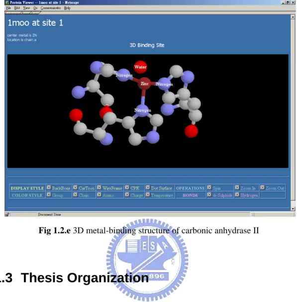
(16) insulin. Metal ions can also serve as redox centers for catalysis, such as heme-iron centers, copper ions and non-heme irons. Other metal ions can serve as electrophilic reactants in catalysis, as in the case of active site zinc ions of the metalloprotease. For example, the enzyme carbonic anhydrase (Figure 1.2.e) typically forms 4 coordinate bonds in a tetrahedral arrangement about its metal ion.. Enzyme Class Distribution Biological level. Element. bulk element. trace element. possible trace element. N/A. Ca Mg Na K Zn Fe Mn Se Cu Co Ni I Mo V Cr As Hg Cd Al U Cs Pb Pt Tl Be Sm Sr W Yb Au Ho Ba Ag Eu Gd In Li Rb Te La Tb. EC 2 EC 3 EC 4 EC 5 EC 6 EC 1 Oxidoreductases Transferases Hydrolases Lyases Isomerases Ligases 125 38 16 27 101 415 39 34 95 6 10 10 20 9 0 26 8 10 1 3 0 0 1 0 0 1 0 0 0 0 0 0 0 0 0 0 0 0 1 0 0. 74 183 102 32 87 6 65 33 1 10 2 7 0 2 4 7 7 12 5 2 2 2 1 1 2 1 2 1 1 0 2 2 0 1 0 0 0 0 0 0 0. 571 133 257 24 312 15 41 36 8 31 35 18 1 4 0 9 16 26 9 2 1 1 2 3 2 1 2 3 2 2 1 0 1 0 1 0 0 1 0 0 0. 19 45 29 18 125 12 6 17 4 10 3 1 0 0 0 1 55 1 0 0 2 4 1 0 0 1 0 0 1 0 0 0 0 0 0 1 1 0 0 0 0. Table 1.2.c enzyme distribution in metalloprotein. 7. 4 15 22 0 12 1 12 9 0 14 2 2 0 1 0 1 0 2 1 0 1 0 0 0 0 0 0 0 0 1 0 0 0 0 0 0 0 0 0 0 0. 1 44 1 11 19 0 14 5 0 0 0 0 0 0 0 0 0 0 1 1 1 0 0 1 0 0 0 0 0 0 0 0 0 0 0 0 0 0 0 0 0.

(17) Fig 1.2.e 3D metal-binding structure of carbonic anhydrase II. 1.3 Thesis Organization The organization of this thesis is described as follows. First, chapter 2 is involved in the biological resource building and sequence data processing. Chapter 3 is concerned about the algorithms on metal binding residue prediction and Chapter 4 is the results and discussion about prediction. Appendix is a simple manual for bioinformatics tool or protocol in the thesis.. 8.

(18) Chapter 2 Biological Resource In this chapter, there are three issues are concerned. Section 2.1 shows how to obtain proper biological reference for demand. Further, section 2.2 gives an example to design a self-defined database for target data storage fitted to actual protein metal-binding model. Finally, section 2.3 shows the biological data processing and sampling.. 2.1 Integration of Web Biological Databases The main data resources come from two web sites; one is the metalloprotein database and browser (MDB) of metalloprotein structure and design program of the Scripps Research Institute (http://metallo.scripps.edu). Another one is Protein Data Bank (PDB, http://www.rcsb.org/pdb/), which provides general information about every protein structure. Hence, by combing these two data sets, the detail description of metalloprotein can be driven. For simplicity, the PDB information can be replaced by another compacted data － PDBFinder (http://www.cmbi.kun.nl/gv/pdbfinder/) released at September, 14, 2003.. In MDB, all proteins with binding metal can be entirely extracted and the binding site is also defined by nearby amino acid residues and compounds in order to develop a sufficient understanding about metalloproteins. To achieve this, it is needed to comprehend the set of structural, environmental, and functional requirements for metal-binding sites in existing metalloprotein or metalloenzymes. In structure, MDB has catalogued several important issues, such as what types of (metal) ions are bound to protein molecule, what types of ligands that bind these metal ions (i.e. the first-shell ligands), and what residues that contact the metal-binding ligands (i.e. the second-shell ligands) as illustrated in Figure 2.1.a.. 9.

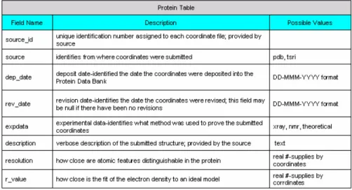
(19) As the result, there are three tables (As shown in Table 2.1.a to Table 2.1.c) － Protein Table, Site Table and Ligand Table needed to describe the structural relationship between protein and metal binding site in nature. That is to say, the objective can be translated as discovering the metal-binding second-shell ligands (residues) from protein primary structure (protein amino acid sequence).. Fig 2.1.a Metal-Ligand diagram in metal-binding protein. Table 2.1.a Protein Table in MDB. 10.

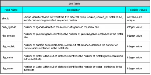
(20) Table 2.1.b Site Table in MDB. Table 2.1.c Ligand Table in MDB But these databases are not directly released to public. Only available information is formatted into 43 ligand text files with respect to 43 kind different binding metals. The latest version of file package is “18” and is updated at January, 17, 2003. The following Figure 2.1.b shows the format of ligand file.. Fig 2.1.b Format of ligand file in MDB package. Each line in file represents one binding site surrounded by one center atom in protein. The file format of each line in ligand file can be expressed as 11.

(21) N. [protein information] + [center information] + [number of ligands (N)] +. ∑ [ligand information] i=1. The term protein information is the file name of PDB file, noted as unique PDB ID tailed with “.pdb.” The second term is the information about metal center which is one text with 5 fields － type of central atom, recognition type (A or H) of central atom, protein chain identifier where central atom located, residue series number of central atom located, and symbol of central atom. In recognition type, if it shows “A” then the central element is recognized as atom of standard residue; else if it shows “H” then it is recognized as atom of non-standard group in protein.. The third term is an integer number which indicates the number of binding ligands (assume to be N for illustration) with respect to this central atom. After this term, there are N ligands information follow. In ligand (binding atom) information, there are 7 fields involved － type of binding atom (P, N, M, W, A or H), recognition type of binding atom (A or H, the same as central atom recognition rule), protein chain identifier where binding atom located, residue name where binding atom located, residue series number of binding atom located, symbol of binding atom and distance (in angstrom) between central atom and binding atom. In binding atom type, if it shows “P”, “N”,”M”, “W”, “A” or “H’ then the type of binding atom is classified as atom of protein, atom of nucleic acid, metal atom, atom of water molecule, anion (negatively charged ion) or hetero atom. It is very useful when searching for metal binding residue (recognition type is ‘A’) in database.. In the similar way, PDB or PDBFinder database is released in the form of text files or accessed from html browser. For efficiency, it is necessary to build stand-alone database on local machine by parsing these released files. Therefore, each field in text file must be identified and clarified. In PDBFinder, there are three major levels of information about － (1) entire protein, (2) each one chain in protein and (3) hetero group of entire protein.. Level (1) PROTEIN provides several important messages about whether this protein is enzyme or not, the experimental details in determining this protein 12.

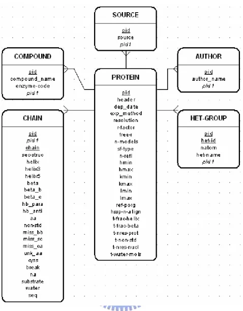
(22) structure and statistics on total number of aligned sequences in HSSP (database of Homology-derived Secondary Structure of Proteins), fraction of helix or beta sheet (major secondary structures), total umber of amino acid residues (standard and non-standard), total number of nucleic acids in protein, and total number of water molecules.. Level (2) CHAIN offers detailed description of each chain in protein, such as statistics about secondary structures (helix, 3/10 helix, pi helix, beta sheet, beta bridges, extended bridges, number of parallel and anti-parallel strand hydrogen bonds), amino acids (number of standard amino acids, number of non-standard amino. acids,. number. of. backbone-missing. amino. acids,. number. of. sidechain-missing amino acids, number of only-Ca-given amino acid, number of unknown amino acids, number of Cystine residues, and number of chain-break which is larger than 4.5 angstrom) number of nucleic acids, number of enzyme substrate, number of water molecule, and primary structure sequence in this chain.. Level (3) HET-Groups show hetero group information as records in PDB file headed by HET. Table 2.1.d, 2.1.e and 2.1.f shows tree organization of records in level (1), (2), and (3) respectively. By combining these databases, the binding site of each protein can be extracted and it is possible to classify all proteins into enzyme or non-enzyme groups. Figure 2.1.c shows one example in PDBFinder released file. Because the details about PDB file format is too verbose so that it is described in appendix.. 13.

(23) Layer 1. Layer 2. Layer 3. Location. Meaning/Note. ID. Possible value/Data type. 4-letter PDB code. 4 letters. Header. PDB Header. PDB Header. Text. Date. PDB Header. Deposition date. Text. Compound. PDB COMPND. PDB COMPND. Text. Enzyme-code. PDB COMPND. EC number. X.X.X.X, (X is one integer). Source. PDB SOURCE. PDB SOURCE. Text. Author. PDB Author. Authors’ names. Text. PDB EXPDTA. Experiment methods. {X, NMR, FIBER, MODEL, NEUTRON, OTHER}. Header. Compound. Exp_Method Resolution R-factor Exp_Method. PDB REMARK. X-ray only. Text. R-factor. REMARK3, 4. X-ray only. Real number. Free-R. REMARK3. X-ray only. Real number. PDB MODEL. # of NMR models. Integer. N-Models SF-Type. Structure factors file type. PDB, CIF, Unknown. N-refl. # of reflections. Integer. H-min, H-max. H index of reflection. Integer. K-min, K-max. K index of reflection. Integer. L-min, L-max. L index of reflection. Integer. Ref-Prog. Names of refinement programs. Text. HSSP-N-Align. # of aligned sequences in HSSP. Integer. T-Frac-Helix, Beta. Total fraction of helix or beta. Integer. T-Nres_Prot. T-Nres_Prot. Total # of AA residues within the protein, including non standard. Integer. T-non-std. SF-Type. Total # of non-standard residues. Integer. T-Nres-Nucl. Total # of NA residues. Integer. T-Water-Mols. Total # of water molecules. Integer. Table 2.1.d Record organization in level (1) PROTEIN. Layer 1. Layer 2. Layer 3. Layer 4. Location. Chain Sec-Struc. Possible value/Data type Text. # of residues which has SS. Integer. Helix. # of residues which are helix. Integer. i, i+3. # of residues which are 3/10 helix. Integer. i, i+5. # of residues which are pi helix. Integer. Beta. # of residues which are beta. Integer. B-Bridge. # of residues which are beta bridge. Integer. E-beta. # of residues which are extended bridge. Integer. Para-Hb. # of parallel strand Hydrogen bonds. Integer. Anti-Hb. # of anti-parallel strand Hydrogen bonds. Integer. Amino-Acids. # of AA residues, including non-standard. Integer. Non-Std. # of non-standard AA. Integer. Miss-BB. # of backbone-missing AA. Integer. Miss-SC. # of sidechain-missing AA. Integer. Only-Ca. # of only-CA-given AA. Integer. UNK. # of unknown type AA. Integer. CYSS. # of Cys residues, it’s about SS bond. Integer. Break. # of chain breaks (> 4.5 A). Integer. Nucl-Acids. # of NA. Integer. Substrate. # of substrate atoms. Integer. Water-Mols. # of water molecules. Integer. Sequence. 1-letter code of AA or NA. Text. Helix. Sec-Struc. Beta. Chain. AminoAcids. From DSSP. Meaning/Note Protein polymer Chain ID. Table 2.1.e Record organization in level (2) CHAIN. 14.

(24) Layer 1. HET-Groups. Layer 2. Location. HET-Groups. PDB HET. Meaning/Note. Possible value/Data type. # of HET groups. Integer. Het-Id. HET residue series number. Integer. Natom. # of atoms within each HET group. Integer. Name. Full name of HET group. Text. Table 2.1.f Record organization in level (3) HET-Groups • • • • • • • • • • • • • • • • • • • • • •. HET-Groups : 7 Het-Id :9 Natom :1 Name : SILVER ION Het-Id : 14 Natom :1 Name : SILVER ION Het-Id : 20 Natom :1 Name : SILVER ION Het-Id : 26 Natom :1 Name : SILVER ION Het-Id : 30 Natom :1 Name : SILVER ION Het-Id : 36 Natom :1 Name : SILVER ION Het-Id : 38 Natom :1 Name : SILVER ION. • • • • • • • • • • • • • • •. ID : 1AOO Header : METALLOTHIONEIN Date : 1997-07-08 Compound : ag-metallothionein Compound : (ag-mt) Compound : biological_unit: monomer; Source : (saccharomyces cerevisiae) Source : baker's yeast Author : C.W.Peterson Author : S.S.Narula Author : I.M.Armitage Exp-Method : NMR Ref-Prog : X-PLOR HSSP-N-Align : 3 T-Nres-Prot : 40. • • • • •. Chain :_ Sec-Struc : 40 Amino-Acids : 40 Substrate : 7 Sequence : QNEGHECQCQCGSCKNNEQCQKSCSCPTGCNSDDKCPCGN. Fig 2.1.c an example of released text file in PDBFinder. 2.2 Metal Binding Model and Database Design Since in section 2.1 all fields in each released text file of target have been identified. Next step is to build a “container” for these biological data. Figure 2.2.a and Figure 2.2.b shows the DSD (Data Structure Definition) schematics of PDBFinder and MDB. Abstractly, the data hierarchy can be defined as 4 layers ordered by their size. They are PROTEIN, CHAIN, SITE and LIGAND. The top level PROTEIN may contain one or several chain (s), and each chain is represented as one polypeptide chain belonged to one protein in nature. Every site contains the coordinate information about entire metal center binding site, just like shown in Fig 1.2. The environment information describes about how many binding atoms (ligands) participate in the site, which residue the ligand located, and what these binding ligands are. The binding hierarchy model and ERD (Entity-Relationship Diagram) is shown in Figure 2.2.c and Figure 2.2.d. 15.

(25) Fig 2.2.a DSD schematic of PDBFinder. Fig 2.2.b DSD schematic of MDB. 16.

(26) Site 1 of Chain A. Site 1 of Chain B. Chain B. Chain A. Site 2 of Chain B Site 2 of Chain A. One protein. Metal center Binding ligand (atom). One Site. Binding residue or molecule. Fig 2.2.c Metal-binding protein data hierarchy. 17.

(27) Fig 2.2.d Entity Relationship diagram of PDBFinder and MDB. 2.3 Biological Data Processing and Sampling In this thesis, there are 43 elements concerned in MDB version 17 as shown in Table 2.3.a. After cross querying between MDB and PDBFinder by scripts written in network programming language PHP (http://www.php.net/) on local MySQL (http://www.mysql.com) database, 41 and 35 metal types can be found in protein and enzyme respectively. Table 2.3.b shows the list of elements in metal binding residue prediction after cross querying. For simplicity, each instance in integrated database is treated as one chain of protein in real world; as the result, the inter-chain metal binding won’t be considered. By binding information from MDB, every position in protein chain sequence can be marked as binding or non-binding to be input for learn scheme (in chapter 3). Figure 2.3.a concludes all demanded data process and flow. 18.

(28) Fig 2.3.a Data processing pipeline In Table 2.3.b, the first column indicates biological level which is the classification of life element in [3]. The third column is the element classification from periodic table. Next two columns are total number of metal binding chains in protein and enzyme. From existence of the field “EC_number” in entity “compound” of database PDBFinder, it is easy to identify whether a protein is an enzyme or not. The last column is the ratio of enzyme and all terms are ordered by this ratio. Element Number of sites (Lines in ligand file) Mg 6161 Fe 5357 Se 4861 Ca 4409 Zn 3326 Na 2018 Mn 1584 W 1065 Cu 849 Cd 813 U 788 K 784 Hg 465 I 416 Co 395 Ni 257 As 186 Mo 102 Al 76 Cs 71 Tl 59. Element Ho Sr Sm V Pb Pt Au Gd Ba Yb Be Cr Ag Rb Rh La Te Eu Tb Si Li In. Ordered by number of sites w.r.t. element type. Number of sites (Lines in ligand file) 53 53 52 52 46 41 35 29 26 26 25 23 15 15 15 11 8 7 7 5 3 2 Sum : 34591. Table 2.3.a Number of site in MDB released files. 19.

(29) Fig 2.3.b Life elements in periodic table. Figure 2.3.b illustrates all life elements in periodic table in biological system., and there are 11 bulk biological elements－hydrogen (H), carbon (C), nitrogen (N), oxygen (O), sodium (Na), magnesium (Mg), phosphorus (P), sulfur (S), chlorine (Cl), potassium (K), and calcium (Ca), 12 trace elements essentials for life－ vanadium (V), chromium (Cr), manganese (Mn), iron (Fe), cobalt (Co), nickel (Ni), copper (Cu), zinc (Zn), selenium (Se), molybdenum (Mo), tin (Sn), and iodine (I) and 2 possible trace elements－arsenic (As) and bromine (Br) in periodic table as indicated in [4]. After cross comparison, there are 4 of 11 (36%) bulk biological elements, 11 of 12 (91.6%) trace elements, and 1 of 2 (50%) possible trace elements in MDB as shown in Table 2.3.b which is classified by their biological level and order by their enzyme-protein ratio (E/P, the last column) with respect to each biological level set.. Owing to avoiding bias phenomenon of homology sequences in sets corresponding to different metal elements, sequence identity check has been applied to eliminate redundant sequence from each set. Table 2.3.c and Table 2.3.d show the set size comparison between different sets with respect to binding metal under different sequence identity thresholds. The selection criteria is when the average sequence identity of one chain to all sequences in the set except itself is less than the sequence identity threshold, the sequence is chose under this threshold. Before computing the pairwise sequence identity, all sequences in set are aligned by multiple sequence alignment (MSA) software － Clustalw. Single chain subset is skipped and noted the number of chain as “n/a (not available).”. 20.

(30) biological level. element name. chains in Protein. chains in Enzyme. E/P. 243. 175. 72.02%. 707. 450. 63.65%. 1738. 785. 45.17%. Ca. 2455. 1018. 41.47%. Cr. 6. 6. 100.00%. K bulk element. Alkaline metal. V. 12. 10. 83.33%. Co. 174. 97. 55.75%. Mo. 48. 24. 50.00%. 172. 85. 49.42%. Zn. 2329. 1064. 45.68%. Mn. 956. 400. 41.84%. Ni. possible trace element. Alkali metal. Na Mg. trace element. element type. Transition metal. Cu. 567. 213. 37.57%. Fe. 2795. 803. 28.73%. Se. Non-metal. 16. 12. 75.00%. I. Halogen. 15. 6. 40.00%. As. Semi-metal. 79. 51. 64.56%. 221. 103. 46.61%. Hg Ag. 3. 1. 33.33%. Cd. 267. 80. 29.96%. 7. 2. 28.57%. W. 7. 2. 28.57%. U. 63. 14. 22.22%. Au. 14. 2. 14.29%. Tb. 1. 0. 0.00%. 4. 2. 50.00%. Yb. 14. 7. 50.00%. Eu. 2. 1. 50.00%. 6. 1. 16.67%. Sm. 20. 3. 15.00%. Gd. 16. 0. 0.00%. La. 5. 0. 0.00%. Tl. 18. 18. 100.00%. 22. 17. 77.27%. Pb. 22. 7. 31.82%. In. 1. 0. 0.00%. Ba. 3. 2. 66.67%. 12. 3. 25.00%. 6. 0. 0.00%. 7. 4. 57.14%. 2. 1. 50.00%. 1. 0. 0.00%. Pt. Te. Ho n/a. Al. Sr. Transition metal. Semi-metal. Rare Earth. Basic metal. Alkaline metal. Be Cs Li. Alkali metal. Rb. Table 2.3.b Number of chains in protein set and enzyme set after cross querying. 21.

(31) Sequence Identity Threshold biological level. bulk element. trace element. possible trace element. n/a. element Total chains in protein. 75%. 50%. 25%. 10%. R. R/T. R. R/T. R. R/T. R. R/T. Ca. 2455. 2455. 100.00%. 2455. 100.00%. 2455. 100.00%. 2322. 94.58%. Mg. 1738. 1738. 100.00%. 1738. 100.00%. 1738. 100.00%. 1738. 100.00%. Na. 707. 707. 100.00%. 707. 100.00%. 707. 100.00%. 547. 77.37%. K. 243. 243. 100.00%. 243. 100.00%. 243. 100.00%. 173. 71.19%. Fe. 2795. 2795. 100.00%. 2795. 100.00%. 2795. 100.00%. 2241. 80.18%. Zn. 2329. 2329. 100.00%. 2329. 100.00%. 2329. 100.00%. 2329. 100.00%. Mn. 956. 956. 100.00%. 956. 100.00%. 956. 100.00%. 706. 73.85%. Cu. 567. 567. 100.00%. 567. 100.00%. 567. 100.00%. 307. 54.14%. Co. 174. 174. 100.00%. 174. 100.00%. 174. 100.00%. 129. 74.14%. Ni. 172. 172. 100.00%. 172. 100.00%. 172. 100.00%. 99. 57.56%. Mo. 48. 48. 100.00%. 48. 100.00%. 13. 27.08%. 6. 12.50%. Se. 16. 16. 100.00%. 7. 43.75%. 7. 43.75%. 1. 6.25%. I. 15. 15. 100.00%. 15. 100.00%. 15. 100.00%. 5. 33.33%. V. 12. 12. 100.00%. 5. 41.67%. 3. 25.00%. 0. 0.00%. Cr. 6. 0. 0.00%. 0. 0.00%. 0. 0.00%. 0. 0.00%. As. 79. 79. 100.00%. 21. 26.58%. 21. 26.58%. 9. 11.39%. Cd. 267. 267. 100.00%. 267. 100.00%. 267. 100.00%. 267. 100.00%. Hg. 221. 221. 100.00%. 221. 100.00%. 154. 69.68%. 128. 57.92%. U. 63. 63. 100.00%. 32. 50.79%. 32. 50.79%. 17. 26.98%. Al. 22. 22. 100.00%. 22. 100.00%. 10. 45.45%. 1. 4.55%. Pb. 22. 22. 100.00%. 22. 100.00%. 22. 100.00%. 4. 18.18%. Sm. 20. 20. 100.00%. 20. 100.00%. 12. 60.00%. 6. 30.00%. Tl. 18. 18. 100.00%. 6. 33.33%. 2. 11.11%. 0. 0.00%. Gd. 16. 16. 100.00%. 16. 100.00%. 10. 62.50%. 1. 6.25%. Au. 14. 14. 100.00%. 14. 100.00%. 10. 71.43%. 0. 0.00%. Yb. 14. 14. 100.00%. 14. 100.00%. 14. 100.00%. 1. 7.14%. Sr. 12. 12. 100.00%. 12. 100.00%. 12. 100.00%. 1. 8.33%. Cs. 7. 7. 100.00%. 7. 100.00%. 3. 42.86%. 0. 0.00%. Pt. 7. 7. 100.00%. 7. 100.00%. 7. 100.00%. 0. 0.00%. W. 7. 7. 100.00%. 7. 100.00%. 7. 100.00%. 0. 0.00%. Be. 6. 0. 0.00%. 0. 0.00%. 0. 0.00%. 0. 0.00%. Ho. 6. 6. 100.00%. 4. 66.67%. 1. 16.67%. 0. 0.00%. La. 5. 5. 100.00%. 5. 100.00%. 1. 20.00%. 0. 0.00%. Te. 4. 4. 100.00%. 0. 0.00%. 0. 0.00%. 0. 0.00%. Ag. 3. 3. 100.00%. 1. 33.33%. 0. 0.00%. 0. 0.00%. Ba. 3. 3. 100.00%. 1. 33.33%. 0. 0.00%. 0. 0.00%. Eu. 2. 2. 100.00%. 0. 0.00%. 0. 0.00%. 0. 0.00%. Li. 2. 2. 100.00%. 0. 0.00%. 0. 0.00%. 0. 0.00%. In. 1. Rb. 1. Tb. 1. n/a. Table 2.3.c Protein set size under different sequence identity threshold. 22.

(32) Sequence Identity Threshold biological level. bulk element. trace element. possible trace element. n/a. element Total chains in enzyme. 75%. 50%. 25%. 10%. R. R/T. R. R/T. R. R/T. R. R/T. Ca. 1018. 1018. 100.00%. 1018. 100.00%. 1018. 100.00%. 892. 87.62%. Mg. 785. 785. 100.00%. 785. 100.00%. 785. 100.00%. 661. 84.20%. Na. 450. 450. 100.00%. 450. 100.00%. 450. 100.00%. 245. 54.44%. K. 175. 175. 100.00%. 175. 100.00%. 175. 100.00%. 100. 57.14%. Zn. 1064. 1064. 100.00%. 1064. 100.00%. 1064. 100.00%. 994. 93.42% 93.77%. Fe. 803. 803. 100.00%. 803. 100.00%. 803. 100.00%. 753. Mn. 400. 400. 100.00%. 400. 100.00%. 400. 100.00%. 222. 55.50%. Cu. 213. 213. 100.00%. 213. 100.00%. 182. 85.45%. 79. 37.09%. Co. 97. 97. 100.00%. 97. 100.00%. 97. 100.00%. 48. 49.48%. Ni. 85. 85. 100.00%. 85. 100.00%. 66. 77.65%. 23. 27.06%. Mo. 24. 24. 100.00%. 16. 66.67%. 11. 45.83%. 0. 0.00%. Se. 12. 3. 25.00%. 3. 25.00%. 3. 25.00%. 0. 0.00%. V. 10. 10. 100.00%. 3. 30.00%. 1. 10.00%. 0. 0.00%. I. 6. 6. 100.00%. 6. 100.00%. 4. 66.67%. 0. 0.00%. Cr. 6. 0. 0.00%. 0. 0.00%. 0. 0.00%. 0. 0.00%. As. 51. 11. 21.57%. 11. 21.57%. 11. 21.57%. 5. 9.80%. Hg. 103. 103. 100.00%. 103. 100.00%. 63. 61.17%. 41. 39.81%. Cd. 80. 80. 100.00%. 80. 100.00%. 80. 100.00%. 58. 72.50%. Tl. 18. 18. 100.00%. 6. 33.33%. 2. 11.11%. 0. 0.00%. Al. 17. 17. 100.00%. 17. 100.00%. 7. 41.18%. 0. 0.00%. U. 14. 14. 100.00%. 14. 100.00%. 4. 28.57%. 0. 0.00%. Pb. 7. 7. 100.00%. 7. 100.00%. 2. 28.57%. 0. 0.00%. Yb. 7. 7. 100.00%. 7. 100.00%. 0. 0.00%. 0. 0.00%. Cs. 4. 4. 100.00%. 2. 50.00%. 0. 0.00%. 0. 0.00%. Sm. 3. 3. 100.00%. 1. 33.33%. 0. 0.00%. 0. 0.00%. Sr. 3. 3. 100.00%. 3. 100.00%. 0. 0.00%. 0. 0.00%. Au. 2. 2. 100.00%. 0. 0.00%. 0. 0.00%. 0. 0.00%. Pt. 2. 2. 100.00%. 0. 0.00%. 0. 0.00%. 0. 0.00%. W. 2. 2. 100.00%. 0. 0.00%. 0. 0.00%. 0. 0.00%. Te. 2. 0. 0.00%. 0. 0.00%. 0. 0.00%. 0. 0.00%. Ba. 2. 0. 0.00%. 0. 0.00%. 0. 0.00%. 0. 0.00%. Ho. 1. Ag. 1. Eu. 1. Li. 1. Gd. 0. Be. 0. La. 0. In. 0. Rb. 0. Tb. 0. n/a. Table 2.3.d Enzyme set size under different sequence identity threshold. 23.

(33) Chapter 3 Machine Learning Scheme The learning schemes used, in this thesis, are as simple as possible so that it becomes easy to observe the prediction performances according to various coding using non-biological or biological features. Besides, the relationship between the performance and size of sequence sampling window also can be found.. 3.1 Neural Networks Neural network consist of groups of parallel processing unit with connection between layers and each connection has one weight parameter. Neural networks use these weights between layers to “memorize” the patterns fed from input layer. The basic unit within a layer is an artificial neuron (node) shown as one circle in Figure 3.1.a. In this thesis, multi-layer Perceptron (MLP) neural networks with back-propagation (BP) algorithm are chosen as learning machine to complete our experiments. In the NNs, we used one hidden layer with 30 hidden nodes as shown in Figure 3.1.a so that there are (30 × dimension of input layer) weights between input layer and hidden layer and (30 × dimension of output layer) weights between hidden layer and output layer respectively.. Fig 3.1.a simple full connection neural networks. Besides, dimension of input layer is depended on the size of sequence sample 24.

(34) window and dimension of output layer is two. In testing phase, if first output value is larger than second one, then the prediction result is defined as positive (binding), otherwise negative (non-binding).. 3.2 Feature Encoding There are two input coding used in our experiments. One is direct one-hot coding which presents every amino acid as one 21-bits array. Only one bit in array is ‘1’ and other bits in array are ‘0’.. In this way, every type of natural amino acid can be. indicated by the position of the only “1” bit. Owing to the unknown type (usually use the symbol ‘X’ in sequence) of amino acid in protein sequence, add one bit to record this condition. This is the non-biological coding for amino acid as illustrated in Table 3.2.a.. Table 3.2.a One-hot coding table for 20 amino acids Another coding method is done by referencing five different types of biological features about amino acid as shown in Table 3.2.b. and Table 3.2.c.. 25.

(35) Feature Set (size). Definition and Content. Physical (3). mass, volume, and area. Solvent Exposed Area Levels (3). three levels. Hydrophobicity Scales (6). six scales. Secondary Structure Propensity (3). three secondary structures. Chemical Classification (8). eight classifications. References 7. NCBI statistics. SEA > 30 10 < SEA < 30 SEA < 10 Engleman-Steitz Hopp-Woods Kyte-Doolittle Janin Chothia Eisenberg Weiss Alpha helix Beta strand Turn (loop, coil) Polar Non-Polar Charged Positive Tiny Small Aromatic Aliphatic. [8] [9] [10] [11] [12] [13] [14] [1]. [7]. Table 3.2.b Definitions of five biological feature sets. Table 3.2.c Values of five biological feature sets Because the binding behavior of central metal atom is influenced by the surrounding environment in protein, it is necessary to observe in wider scope than 7. National Biotechnology Information Center, U.S.A. http://www.ncbi.nlm.nih.gov/ 26.

(36) single one amino acid so as to determine whether the binding happens or not. Accordingly, each input vector applied to learning machine is extracted from one segment of entire chain by the concept － continuous sliding window. Each sliding window is centered by the “target” amino acid. And the rest of the amino acids in window are the “neighbors” of the target. Figure 3.2.c shows the feature extraction, learning scheme and how sliding window works. For simplicity the window size illustrated is 5.. Fig 3.2.c Feature extraction, learning scheme and sliding window. 27.

(37) Chapter 4 Results and Conclusion In out experiments, there are two major sets － protein and enzyme sets with specified sequence identity constraint. To avoid sampling bias, the sequence identity threshold is set as 25% － the threshold of homology modeling. Each set corresponding to different metal element has its own neural network which is trained for 150 epochs to observe its time-varied characteristics. Five fold cross validation is used to calculate performance, shown in Fig 4.a.. Fig 4.a five fold cross validation. 28.

(38) 4.1 Performance Measures Four basic performance measures are used in the experiment － TP (true positive, when an instance (residue) is observed as positive, and predicted as positive), TN (true negative, when an instance is observed as negative, and predicted as negative), FP (false positive, when an instance is observed as negative, but predicted as positive), and FN (false negative, when an instance is observed as positive, but predicted as negative).. Besides, three performance measures, Qtotal (Equation 1), Qpredicted (Equation 2) and Qobserved (Equation 3), are also used in our experiments. Qpredicted is defined as the ratio between the “true” and total (true and false) instances predicted as positive (binding) and it also shows that how likely the result of prediction would be true when an instance predicted as positive. Qobserved is defined as the ratio between the instances truly predicted as positive and instances observed as positive and it also shows the ability to discover binding residues so that it is also called “sensitivity.” More detailed performance measures and comparison are listed in Table 4.1. Qtotal =. TP + TN TP + TN + FP + FN. TP TP + FP TP = TP + FN. (1). Q predicted =. (2). Qobserved. (3). TABLE 4.1 DETAILED PERFORMANCE MEASURES AND COMPARISON. 29.

(39) 4.2 Experiments on One-hot Coding Method In this section, one-hot coding method is used in all experiments varied by size of window from 5 to 17 so as to observe the change of performance according to different window size. Owing to the extremely low P/N (positive and negative instance ratio), specificity and negative prediction rate (almost approach 100%) are relatively higher than sensitivity (Q-observed). As the result, sensitivity (Q-observed) becomes only one critical term in performance measures in these absolutely unbalanced (positive and negative) training. Table 4.2.a shows all Q-observed in enzyme set with respect to different window size. Figure 4.2.a and Figure 4.2.b offer detailed comparison in bulk and trace elements respectively.. biological level. Bulk element. Trace element. Possibly Trace element. N/A. element Ca K Mg Na Co Cr Cu Fe I Mn Mo Ni Se V Zn As Al Au Ba Cd Cs Hg Pb Pt Sm Sr Te Tl U W Yb. 5. 7. 9. window size 11. 13. 15. 17. P/N. 21.01% 2.99% 8.50% 9.59% 31.43% 0.00% 32.73% 40.40% 0.00% 21.94% 0.00% 42.42% 0.00% 0.00% 24.22% 25.00% 0.00% 0.00% 0.00% 31.08% 0.00% 29.73% 50.00% 0.00% 0.00% 0.00% 0.00% 62.50% 42.86% 0.00% 0.00%. 17.31% 14.93% 10.46% 13.01% 34.29% 0.00% 33.64% 35.82% 25.00% 31.12% 0.00% 42.42% 0.00% 0.00% 15.74% 25.00% 10.00% 0.00% 0.00% 30.41% 0.00% 43.24% 50.00% 0.00% 0.00% 0.00% 0.00% 87.50% 42.86% 0.00% 0.00%. 16.13% 17.91% 12.09% 13.70% 35.71% 0.00% 41.82% 35.82% 62.50% 29.08% 0.00% 51.52% 0.00% 0.00% 14.19% 25.00% 80.00% 0.00% 0.00% 37.16% 0.00% 45.95% 58.33% 0.00% 0.00% 0.00% 0.00% 87.50% 85.71% 0.00% 0.00%. 16.47% 23.88% 10.46% 19.18% 45.71% 0.00% 42.73% 36.39% 75.00% 33.16% 0.00% 54.55% 0.00% 0.00% 24.74% 50.00% 90.00% 0.00% 0.00% 38.51% 0.00% 51.35% 58.33% 0.00% 0.00% 50.00% 0.00% 87.50% 85.71% 0.00% 0.00%. 15.97% 28.36% 13.40% 19.18% 48.57% 0.00% 40.91% 37.25% 75.00% 32.65% 0.00% 51.52% 0.00% 0.00% 29.58% 50.00% 90.00% 0.00% 0.00% 39.86% 0.00% 58.11% 66.67% 0.00% 0.00% 100.00% 0.00% 100.00% 100.00% 0.00% 0.00%. 18.49% 37.31% 14.05% 19.18% 50.00% 0.00% 42.73% 40.40% 75.00% 31.63% 100.00% 54.55% 0.00% 0.00% 27.51% 75.00% 90.00% 0.00% 0.00% 43.92% 20.00% 56.76% 75.00% 0.00% 71.43% 75.00% 0.00% 100.00% 71.43% 0.00% 0.00%. 20.50% 34.33% 18.63% 24.66% 54.29% 0.00% 46.36% 38.40% 87.50% 35.71% 20.00% 63.64% 0.00% 0.00% 30.10% 62.50% 100.00% 0.00% 0.00% 47.30% 60.00% 56.76% 75.00% 0.00% 85.71% 100.00% 0.00% 100.00% 100.00% 0.00% 0.00%. 0.67% 0.46% 0.62% 0.62% 1.25% 1.67% 0.92% 0.62% 0.46% 1.22% 0.95% 1.04% 0.50% 0.51% 0.57% 0.84% 0.19% 0.76% 0.58% 0.52% 0.46% 0.16% 0.90% 0.36% 0.26% 0.88% 0.42% 0.18% 0.38% 0.17% 1.09%. Table 4.2.a Q-observed of 31 elements in enzyme set w.r.t. different window size Increasing window size indeed improves the sensitivity in each metal set; but in some sets, it is not necessary to have better performance with longer window size, 30.

(40) such as in metal sets calcium (Ca) and zinc (Zn). Nevertheless, the large computation cost resulted from the extension of sampling window doesn’t bring great and rapid improvement on performance.. Fig 4.2.a Q-observed of 4 bulk elements by one-hot coding. Fig 4.2.b Q-observed of 11 trace elements by one-hot coding. 31.

(41) Fig 4.2.c Q-observed versus training epoch of bulk elements. Besides, every binding metal specified subset is trained for 100 epochs in experiments and Q-observed training curves are shown as Figure 4.2.c and right-button corner of figure is index table for these subfigures in it. In these subfigures, there are two labels (element name and Q-observed value at 100 epochs) on each training curve. By comparing these curves, one can observe how Q-observed values grow under window extension：. (1) All Q-observed values are not greater than 40% under one-hot coding method in bulk elements. It might be the limitation of one-hot coding method to this problem. 32.

(42) (2) While size of window increases, in general, every training curve rises earlier, and achieves higher Q-observed value at end of training. In addition, the rising edge of curve becomes sharper (curve converges earlier).. (3) Following the last observation in (2) and comparing the curve of four bulk elements, potassium (K) is the most sensitive element than other three elements while window extends.. 33.

(43) 4.3 Comparison between Different Feature sets In last section, the one-hot coding method does not give contented results and computation cost (time and space) after extension of window size is not proportional to the improvement of performance; hence in this section, one-hot coding method is replaced by biological feature sets as shown in Table 3.2.b and Table 3.2.c. Data set focus on four bulk element (calcium, potassium, magnesium and sodium) subsets with less than 25% sequence identity and sliding window size is 15. The comparison between different feature sets is listed in Table 4.3.a. For simplicity, only Q-observed and Q-predicted values are listed in the table.. Feature set Element TP. Q-observed. Q-predicted. K. 160 61. 47471 13054. 25 0. 435 6. 26.89% 91.04%. 86.49% 100.00%. Mg. 100. 53897. 21. 206. 32.68%. 82.64%. Na Ca K. 99 0 0. 19311 47496 13054. 4 0 0. 47 595 67. 67.81% 0.00% 0.00%. 96.12% n/a n/a. Mg. 0. 53918. 0. 306. 0.00%. n/a. Na Ca K. 0 2 0. 19315 47496 13054. 9 0 0. 146 593 67. 0.00% 0.34% 0.00%. 0.00% 100.00% n/a. Mg. 0. 53918. 0. 306. 0.00%. n/a. Na Ca K. 1 120 67. 19315 47491 13054. 9 5 0. 145 475 0. 0.68% 20.17% 100.00%. 10.00% 96.00% 100.00%. Mg. 67. 53895. 23. 239. 21.90%. 74.44%. Na Ca K. 84 594 67. 19314 47496 13054. 1 0 0. 62 1 0. 57.53% 99.83% 100.00%. 98.82% 100.00% 100.00%. Mg. 306. 53918. 0. 0. 100.00%. 100.00%. Na Ca K. 146 110 25. 19315 47495 13054. 0 1 0. 0 485 42. 100.00% 18.49% 37.31%. 100.00% 99.10% 100.00%. Mg. 43. 53918. 0. 263. 14.05%. 100.00%. Na. 28. 19315. 0. 118. 19.18%. 100.00%. Ca 2nd. Phy. SEA. HP. CC. OneHot. TN. FP FN. Table 4.3.a Comparison of one-hot coding and 5 biological sets in bulk elements. 34.

(44) By comparing the Q-observed, physical and solvent exposed area feature sets do not work well in discrimination of metal-binding and non-metal-binding residues, even worst than direct one-hot coding method. Other three biological feature sets (secondary structure propensity, hydrophobicity scales and chemical classification) get better performance than one-hot coding.. These results reflect and correspond to the characteristics of metal-binding chelates, a three dimension cave for metal ion to “reside” in protein and it also can be interpreted as that the formation of metal-binding chelate is highly related to the secondary structure tendency, degree of hydrophobicity and chemical classification of neighboring amino acids of which the entire protein molecule is composed. It is also apparent that metal-binding phenomena don’t be dominated by the physical features of surrounding amino acids only before these experiments began. However, the results in this section have proved this idea true and show that solvent exposed area is not quite highly related to the formation of metal-binding chelates in protein.. Figure 4.3.b and Figure 4.3.c show the comparison between different feature sets in Q-observed and Q-predicted. The major and significant difference of different feature sets is Q-observed as mentioned before. “Chemical Classifications” of amino acids indeed performs better than other feature sets in metal-binding residue prediction when compare their Q-observed together. Figure 4.3.d shows the growth and trend of Q-observed curve with training time for 6 different feature sets (5 biological feature sets and one-hot coding).. From section 4.2 and 4.3, it is clear that biological insight indeed play an important role in prediction the biochemical phenomena in nature. Although one-hot coding is straight-forward idea in feature encoding of 20 amino, it can not completely represent the behavior and characteristics of metal-binding in protein. After these verbose experiments in this thesis, eventually a direct metal-binding prediction method is proposed and proven to be useful and absolutely accurate in proteins binding four bulk elements under 5 fold cross validation.. 35.

(45) Fig 4.3.b Q-observed comparison between different feature sets and bulk elements. Fig 4.3.c Q-predicted comparison between different feature sets and bulk elements. 36.

(46) Fig 4.3.d Q-predicted versus training epoch between different feature sets. 37.

(47) References [1] C. H. Wu and J. W. McLarty, Neural Networks and Genome Informatics, Elsevier Science Ltd, UK, pp. 67-86, 2000. [2] C. T. Lin and C. S. George Lee, Neural Fuzzy Systems, Prentice-Hall, Inc. N.J., U.S.A. 1996. [3] C. Branden and J. Tooze, Introduction to Protein Structure, 2nd edition, Garland Publishing, Inc., New York, pp. 205-220, 1999. [4] M. J. Kendrick, M. T. May, M. J. Plishka, and K. D. Robinson, Metals in Biological System, Ellis Horwood Limited, England, pp. 11-48, 1992. [5] R. A. Copeland, Enzymes A Practical Introduction to Structure, Mechanism and Data Analysis, 2nd edition, Wiley-VHC, Inc, Canada, pp. 42-74, 2000. [6] J. M. Castagnetto, S. W. Hennessy, V. A. Roberts, E. D. Getzoff, J. A. Tainer and M.E. Pique, “MDB: the Metalloprotein Database and Browser at The Scripps Research Institute”, Nucleic Acids Res. ,Vol. 30, No.1 , pp.379-382, 2002. [7] W. R. Taylor, “The Classification of Amino Acid Conservation”, J. Theor. Biol., Vol.119, pp. 205-218, 1986. [8] D. Bordo and P. Argos, “Suggestions for Safe Residue Substitutions in Site-Directed Mutagensis”, J. Mol. Biol. Vol.217, pp. 721-729, 1991. [9] D. M. Engelman, T. A. Steitz, and A. Goldman, ”Identifying nonpolar transbilayer helices inamino acid sequences of membrane proteins”, Annu. Rev. Biophys. Biophys. Chem. Vol.15, pp. 321-353, 1986. [10] T. P. Hoop and K. R. Woods, “Prediction of protein antigenic determinants from amino acid sequences”. Proc Natl Acad Sci, Vol.78, pp.3824, 1981. [11] J. Kyte and R. Doolit, “A Simple Method for Displaying the Hydropathic Character of a Protein”, J. Mol Biol. Vol.157, pp.105-132, 1982. [12] J. Janin, “Surface and Inside Volumes in Globular Proteins”, Nature, Vol. 277, pp.491-492, 1979. [13] C. Chothia, “Hydrophobic bonding and accessible surface area in proteins”, Nature, Vol.248, pp.338-339, 1974. [14] Eisenberg D., Weiss R.M., Terwilliger C.T., Wilcox W., 1982. Hydrophobic moments and protein structure, Faraday Symp. Chem. Soc. 17:109-120. [15] S.Dietmann and C. Frommel, “Prediction of 3D neighbours of molecular surface patches in proteins by artificial neural networks”, Bioinformatics, Vol. 18, No.1, pp. 167-174, 2002. [16] E. Roulet, P. Bucher, R. Schneider, E. Wingender, Y. Dusserre, T. Werner and N. Mermod, “Experimental Analysis and Computer Prediction of CTF/NFI Transcription Factor DNA Binding Sites”, J. Mol. Biol., Vol. 297, pp. 833-848, 2000. [17] I. Jonassen, I. Eidhammer, D. Conklin and W. R. Taylor, “Structure motif discovery and mining the PDB”, Bioinformatics, Vol. 18, No. 2, pp. 362-367, 2001.. 38.

(48) [18] M. Shah, S. Passovets, D. Kim, K. Ellrott, L. Wang, I. Vokler, P. L. Cascio, D. Xu and Y. Xu, “A Computational pipeline for protein structure prediction and analysis at genome scale”, Bioinformatics, Vol. 19, No. 15, pp. 1985-1996, 2003. [19] M. Cline, R. Hughey and K. Karplus, “Predicting reliable regions in protein sequence alignments”, Bioinformatics, Vol. 18, No. 2, pp. 306-314, 2002.. 39.

(49) Appendix [A] MySQL, Apache and PHP The environment of experiments is set up on X86 computer with Microsoft Windows XP OS. User can install all these components (8MySQL database, Apache web server, and 9PHP webpage preprocessor) individually or use integrated tool kit － Foxserv (http://www.foxserv.net/portal.php) to easily set them ready at once on X86 machine with Microsoft windows or Linux.. [B] PDB File Format The full document is available on PDB website and current version is 2.2 (20 December, 1996). Here the document is condensed as tabular representation as shown as follows. There are totally 10 sections shown in Table B.4 in current version, but there are 12 sections in Table B.1 ~ 3 owing to the mergence of sections. Title and Remark sections are combined into Title section. Crystallographic and Coordinate Transformation sections are joined into one section.. In Table B.1 ~ 3, each section contains types several records and the field “EXISTENCE” indicates that record exists mandatorily or optionally and record type. There are 6 record types (Single, Single Continued, Multiple, Multiple Continued, Grouping, and Other). Their differences are shown in Table B.5.. Table B.3 PDB file format overview part 3. 8 9. an world-wide open source database system, http://www.mysql.com/ cross-platform server-side scripting language used to create dynamic web pages, http://www.php.net 40.

(50) Table B.1 PDB file format overview part 1. Table B.2 PDB file format overview part 2 41.

(51) Table B.4 Sections in PDB file. Table B.5 Record types in PDB file. 42.

(52) [C] Clustalw and Blast Here illustrate several important commands about these multiple sequence alignment tools in terminal mode when sequence sampling. Usually you can download “GUI” version from internet but it needs step by step to click buttons on it so as to complete your task. As the result, this section tends to give a practical guide about how to work on batch mode when you use these tools.. When you download the “terminal” version of these tools (always with their source code), you can set it up on various of machines or OS which has C language complier, such as free gcc, g++ from GNU or other commercial compliers. If you use PC with window OS, you can compile it on window command mode environment. If you are work station user, you don’t need to worry about the purchase of complier and environment.. Table C.1 Important commands in BLAST package. Table C.2 Important commands in clustalw package. 43.

(53) Command Line Parameters Classification. Usage. DATA (sequence). VERBS (do things). General Setting. input sequence file. -PROFILE1=prof1.txt. profile 1. -PROFILE2=prof2.txt. profile 2. -OPTIONS. list the command line parameters. -HELP or -CHECK. outline the command line params.. -ALIGN. do full multiple alignment. -TREE. calculate NJ tree.. -BOOTSTRAP(=n). bootstrap a NJ tree (n= number of bootstraps; def. = 1000).. -CONVERT. output the input sequences in a different file format.. -INTERACTIVE. read command line, then enter normal interactive menus. -QUICKTREE. use FAST algorithm for the alignment guide tree. -TYPE=. PROTEIN or DNA sequences. -NEGATIVE. protein alignment with negative values in matrix. -OUTFILE=. sequence alignment file name. -OUTPUT=. GCG, GDE, PHYLIP, PIR or NEXUS. -OUTORDER=. INPUT or ALIGNED. -CASE. LOWER or UPPER (for GDE output only). -SEQNOS=. OFF or ON (for Clustal output only). -SEQNO_RANGE=. OFF or ON (NEW: for all output formats). -RANGE=m,n. sequence range to write starting m to m+n.. -KTUPLE=n. word size. -TOPDIAGS=n. number of best diags.. Fast Pariwise Alignment -WINDOW=n. Slow Pariwise Alignment. Multiple Alignment PARAMETERS (set things). Profile Alignment. Trees. window around best diags.. -PAIRGAP=n. gap penalty. -SCORE. PERCENT or ABSOLUTE. -PWMATRIX=. Protein weight matrix=BLOSUM, PAM, GONNET, ID or filename. -PWDNAMATRIX=. DNA weight matrix=IUB, CLUSTALW or filename. -PWGAPOPEN=f. gap opening penalty. -PWGAPEXT=f. gap opening penalty. -NEWTREE=. file for new guide tree. -USETREE=. file for old guide tree. -MATRIX=. Protein weight matrix=BLOSUM, PAM, GONNET, ID or filename. -DNAMATRIX=. DNA weight matrix=IUB, CLUSTALW or filename. -GAPOPEN=f. gap opening penalty. -GAPEXT=f. gap extension penalty. -ENDGAPS. no end gap separation pen.. -GAPDIST=n. gap separation pen. range. -NOPGAP. residue-specific gaps off. -NOHGAP. hydrophilic gaps off. -HGAPRESIDUES=. list hydrophilic res.. -MAXDIV=n. % ident. for delay. -TYPE=. PROTEIN or DNA. -TRANSWEIGHT=f. transitions weighting. -PROFILE. Merge two alignments by profile alignment. -NEWTREE1=. file for new guide tree for profile1. -NEWTREE2=. file for new guide tree for profile2. -USETREE1=. file for old guide tree for profile1. -USETREE2=. file for old guide tree for profile2. -SEQUENCES. Sequentially add profile2 sequences to profile1 alignment. Seq-Profile Alignment -NEWTREE=. Structure Alignment. Meaning. -INFILE=input.txt. file for new guide tree. -USETREE=. file for old guide tree. -NOSECSTR1. do not use secondary structure-gap penalty mask for profile 1. -NOSECSTR2. do not use secondary structure-gap penalty mask for profile 2. -SECSTROUT={}. {STRUCTURE or MASK or BOTH or NONE} output in alignment file. -HELIXGAP=n. gap penalty for helix core residues. -STRANDGAP=n. gap penalty for strand core residues. -LOOPGAP=n. gap penalty for loop regions. -TERMINALGAP=n. gap penalty for structure termini. -HELIXENDIN=n. number of residues inside helix to be treated as terminal. -HELIXENDOUT=n. number of residues outside helix to be treated as terminal. -STRANDENDIN=n. number of residues inside strand to be treated as terminal. -STRANDENDOUT=n. number of residues outside strand to be treated as terminal. -OUTPUTTREE={}. {nj OR phylip OR dist OR nexus}. -SEED=n. seed number for bootstraps.. -KIMURA. use Kimura's correction.. -TOSSGAPS. ignore positions with gaps.. -BOOTLABELS={}. {node OR branch} position of bootstrap values in tree display. Table C.3 Full commands of clustalw package. 44.

(54)