內嵌界面問題之矩陣分解法

國

立

交

通

大

學

應用數學系

碩

士

論

文

內嵌界面問題之矩陣分解法

Matrix Factorization Method

for the Immersed Boundary problem

研 究 生：謝先皓

指導教授：賴明治 教授

內嵌界面問題之矩陣分解法

Matrix Factorization Method

for the Immersed Boundary Problem

研 究 生：謝先皓 Student：Hsen-Hao Hsieh

指導教授：賴明治 Advisor：Ming-Chih Lai

國 立 交 通 大 學

應 用 數 學 系

碩 士 論 文

A Thesis

Submitted to Department of Applied Mathematics College of Science

National Chiao Tung University in partial Fulfillment of the Requirements

for the Degree of Master

in

Applied Mathematics

June 2008

Hsinchu, Taiwan, Republic of China

i

內嵌介面問題之矩陣分解法

學生：謝先皓 指導教授

：

賴明治 教授

國立交通大學應用數學系﹙研究所﹚碩士班

摘 要

嵌入邊界法(immersed boundary method)是一種模擬不可壓縮流體的數學模 型，他的特色在於解決有無質量的嵌入邊界的情況。而解決嵌入邊界法的問題， 矩 陣 分 解 法 (matrix factorization method) 是 一 種 利 用 類 似 分 部 步 驟 法 (fractional step method)的方法，將嵌入邊界法分解成三個步驟，在前兩個步 驟我們會面對解一個對稱正定的線性系統，在此我們可以利用共軛梯度法 (conjugate gradient method)來解決這個問題。在這份論文之中，我們利用矩 陣分解法來模擬流場通過各種嵌入之物體，包括流過靜止與可動的圓柱、兩個靜 止的圓柱、以及機翼形狀的物體。

ii

Matrix Factorization Method for the

Immersed Boundary Problem

Student : Hsen-Hao Hsieh Advisor : Ming-Chih Lai

Department of Applied Mathematics

National Chiao Tung University

Abstract

The immersed boundary method is a model to simulate a viscous incompressible fluid with immersed massless boundary. It comes from the Navier-Stokes equation of viscous incompressible fluid with the interaction term between the immersed boundary and the fluid. The matrix factorization method is a formulation of immersed boundary method, and the idea is the fractional step method for Navier-Stokes equation. The immersed boundary problem could be factorized to three steps, and the conjugate gradient method can be applied to solve the first and second step. In this paper, we use the matrix factorization method simulate the flow past stationary or movable immersed object, including the flow past a stationary and a moving cylinder, the flow past two stationary cylinders, and the flow past a winglike object.

iii

誌

謝

本篇論文的完成，首先要感謝我的指導老師－賴明治教授。老師帶領我從大 四下學期至今兩年半的時光，領導我走入了數值計算與數學建模這塊領域。每當 我有不解與疑惑的時候，老師總是有耐心的指導我如何去面對問題，挑戰問題， 並且給我正確的學習態度。我印象最深刻的，是當我遇見瓶頸停滯不前的時候， 老師給我的一段話：「做學問就像打網球一樣，一個人開始學網球，絕不是一個 人苦練一年才開始出去參加比賽，一定是邊練邊出去比賽。」使我了解到做學問， 不是從學中做，而是從做中學，讓我對於研究的本質有更深一層的體會。而老師 不僅是學業的傳授者，更是心靈成長的導師。老師給我們的一句銘言：「做人比 做學問更重要。」讓我在鑽研知識的同時，更進一步的思考我們能夠為社會以及 人群做些什麼。學生在此謹致最誠摯的謝意。在研究的過程中，也感謝曾孝捷學 長與陳冠羽學長，給予我的指導與協助，讓我無論在接觸數值分析這塊領域的時 候，或是學習新的程式語言，都給我相當大的幫助。也感謝曾昱豪學長，將自己 做內嵌邊界法的經驗傳授給我，在此獻上最真誠的謝意。 在論文口試期間，承蒙王偉仲教授、洪子倫教授與吳金典助理教授費心審閱 並提供許多寶貴意見，使本論文得以更加完備，學生永銘在心。 此外，我也要感謝曾鈺傑同學、郭乂維同學、陳建明同學、蔡修齊同學以及 胡偉帆同學。在這兩年的研究生涯裡，一直陪伴我走過了最艱難的日子，在我面 對生命中挫折與打擊的時候，始終在我身旁鼓勵著我，在此謝謝他們。 最後，我要感謝我的母親與外婆，是他們悉心的照顧與栽培，才會有今日的 我。願與他們，以及所有在我周圍關心我的人，一同分享此篇論文完成之喜悅與 榮耀。

iv

目

錄

中文提要 ……… i

英文提要 ……… ii

誌謝

……… iii

目錄

……… iv

一、

Introduction ……… 1

二、

Fractional Step Method ……… 2

2.1 Navier-Stokes equation ……… 2

2.2 Staggered grid discretization ……… 2

2.3 Fractional step method ……… 6

2.4 Boundary conditions ……… 10

三、

Matrix Factorization Method ……… 17

3.1 Mathematical formulation ……… 17

3.2 Discretization ……… 18

3.3 Matrix factorization method ……… 21

四、

Numerical Results ……… 23

4.1 Error estimate of fractional step method … 23

4.2 The flow past a cylinder ……… 24

4.3 The flow past two cylinders ……… 27

4.4 The flow past a wing ……… 29

4.5

The flow past an oscillating cylinder ……… 31

五、

Conclusion ……… 33

1

1

Introduction

As we all know, the immersed boundary method has played an important role in the fluid–solid interaction problems. Peskin [7] first introduced the method to simulate the blood flow with an elastic membrane which can be regarded as the immersed boundary in the fluid. He discretizes the flow field with Eulerian grid, and discretizes the immersed boundary with Lagrangian points. The immersed boundary exerts a force on the fluid, and moves with a velocity, so the immersed object can move or be deformed.

The origin fractional step method is introduced by Chorin [1] to solve the incompressible Navier-Stokes equation. Perot [3] regards the fractional step method as a matrix factorization method, and the idea comes from the LU decomposition. The fractional step method can be written in three steps, which the first and second step can be solved by the conjugate gradient method, and the third step is a projection. Taira and Colonius [9] extend the fractional step method from Navier-Stokes equation to immersed boundary problem by observing the symmetric relationship between the discrete interpolation and regularization operators, and also factorize the scheme to three steps. The conjugate gradient method can be applied to the first and second step.

In Section 2, we introduce how to discretize the incompressible Navier- Stokes equations with the staggered marker-and-cell mesh, and review the fractional step method. The detailed matrix forms of each operator are introduced in Section 2.4 with the Dirichlet and the Neumann boundary conditions. In Section 3, we review the immersed boundary method first, and then consider the discretization of the discrete interpolation and regularization operators. The matrix factorization method is introduced in Section 3.3.

The numerical result is shown in Section 4. We can see the second-order temporal accuracy from the error estimate, and the simulation of the flow past a stationary or moving immersed object, including the flow past a stationary and an oscillating cylinder, the flow past two stationary cylinders, and the flow past a winglike object.

2

2

Fractional Step Method

2.1 Navier-Stokes equation

Consider the incompressible Navier-Stokes equations consisting of the momentum and continuity equations as:

∂ 1

∆   0 

where t, , p t, , Re are the velocity vector, pressure, and Reynolds number, respectively. Usually, the initial condition | and the boundary condition | _Ω are known. If we consider that  , t is a two dimensional vertor, that is, , t u , t , v , t , then we can rewrite the incompressible Navier-Stokes equations to:

1

  1

   0

with the initial conditions , , 0 , , , 0 , and the boundary conditions

, , | , , , | .

2.2

Staggered grid discretization

To discretize the equations, refer to [1, 2, 3, 4], we can use the staggered marker-and-cell mesh that introduced by Harlow and Welsh [5] with implicit Crank-Nicolson for the viscous term and explicit second-order Adams-Bashforth for the convective term:

∆ 3 2 1 2 2   0

where , T and are the discrete velocity and pressure. , , and are the discrete convection, gradient, laplacian and divergence operator, respectively. Before introducing how to discretize these terms, we have to know how staggered marker-and-cell mesh can be applied here.

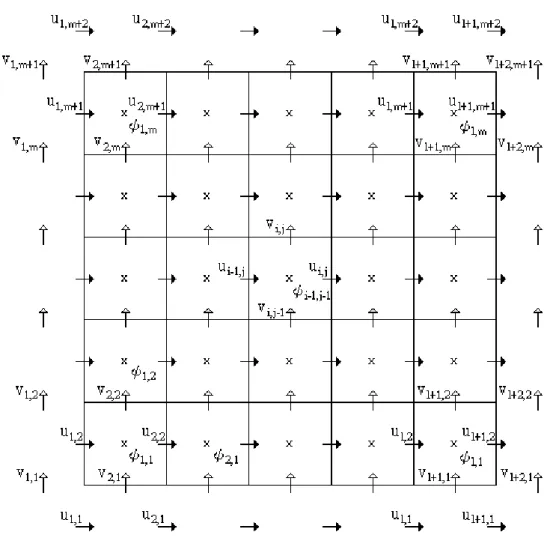
Suppose the two-dimensional domain of this equation is a rectangle. Let the domain Ω 0, X 0, Y , then divide 0, X and 0, Y into parts and parts, respectively. See figure 1, there are cells. To apply the staggered grid discretization to Navier-Stokes equations, we define the discrete velocity of horizontal direction at the center of each cell’s left and right edges, and the discrete velocity of vertical direction at the center of each cell’s upper and lower edges. The discrete pressure is defined at the center of each cell.

Fig. 1. The staggered marker-and-cell mesh

4

To make the scheme simple, suppose ∆ ∆ for all 1 and

1 , then the discrete horizontal velocity _, can be regarded as the

approximation of 1 , 1.5 , . Similarly, the discrete vertical

velocity _, approximates to 1.5 , 1 , and the discrete

pressure _, . approximates to 0,5 , 0.5 , 0.5 .

Use staggered marker-and-cell mesh to discretize the convection, gradient , Laplacian and divergence terms. We can easily obtain the staggered grid discretization of the Navier-Stokes equations. Consider the Laplacian term, using the Taylor expansion, we have

, , , ∆ 1 2! , ∆   , , , ∆ 1 2! , ∆

Add these two formulas, then u , is: , 2 _, ∆ ∆ ∆ 2 _, ∆ ∆ 2 _, ∆ ∆ ∆

Similarly, let ∆ . ∆ ∆ ⁄ , then 2

, 2 _, ∆ _. ∆ _. ∆ _. 2 _, ∆ . ∆ . 2 _, ∆ _. ∆ _. ∆ _.

The discrete Laplacian form can be written as:

Δ _{, , ,}

Since we suppose that ∆ ∆ , we obtain:

Δ , , , 4 , , , ⁄

Similarly,

5

Although the discrete pressure is defined at the center of each cell, is defined at the same place that the discrete velocity and are defined. We use the same index , to represent the discrete _, and _, . Let

∆ _. ∆ ∆ ⁄ The form can be written as: 2

, , , ⁄∆ .   , , , ∆ .  

Consider the convection term. The discretization of the convection term is:

, ,

, ,

∆ ∆ ,

, ,

∆ _. ∆ _.

where _, is the mean of the values of neighbor . That is,

, , , , , 4 Similarly, , , , , ∆ _. ∆ _. , , , ∆ ∆ where , , , , , 4 If ∆ ∆ , then ∆ _. ∆ _.

6

Consider the discrete divergence term. We can use divergence theorem here. Integrate the continuity equation on each cell.

0

 

 

where is the outward normal vector of cell face. Suppose the domain is two-dimensional, then can be rehash to , and can be rehash to or . We obtain the discrete continuity equation:

∆ ∆ _, ∆ _, ∆ 0

, ,

for all 1 and 1 . Since we suppose that ∆ ∆ , it can

be written as:

, , , , 0

2.3

Fractional step method

After discretize the incompressible Navier-Stokes equations, we have to solve the velocity and the pressure . Put the unknown and on the left side of the equal sign, and the other terms on the right side. The discrete formulations of incompressible Navier-Stokes equations are:

1 Δ 1 2 1 Δ 1 2 3 2 1 2                 0

where and are the boundary conditions. The boundary conditions appear in equations because we regard the discrete operators as matrix form,

and both are vectors. Let , and ̂ be the right side of

the momentum equation. That is, ̂ .

7 0

̂

0

The details of the matrix form of the discrete operators could be found in [3]. These matrices will be introduced detailed with the boundary conditions in

Section 2.4, but brief here. First, we define , T and :

, , … , ,    , , … , ,       ,    , , … ,   , , … , ,    , , … , ,       ,    , , … ,   

        _, , … _, ,    _, , … _, ,       ,    _, , … _, Moreover, we define two matrices and :

∆ ∆ 0 0   , ∆ 0 0 ∆ 0 0 ∆ _. ∆ _.  , ∆ _. 0 0 ∆ _.

If ∆ ∆ , then , where is the identity

matrix. We take the discrete momentum equation product , then there is a new matrix form:

̂

8

̂

    

T simpler, let , , ̂, 

o make the matrix form

,   , the matrix form can be written as:

0

There is an interesting fact that T, that is the reason why we rehash the origin matrix form to the new matrix form. The origin fractional step method is introduced by Chorin in [1], Now, we use the fractional step method which is introduced by Perot in [3]. The idea of the fractional step method comes from the LU decomposition:

T T ₀

To handle the inverse matrix of A, there is a approximation introduce by

Témam [16], let , ⁄ , the matrix can be written

as : 1 1 2 1 1 2 1 2

The inverse matrix of can be approximated by :

2 2 2 2 N 

2

N

2 N

N ∑N is the Nth order Talyor expansion of ,

9 T T N N 0 N 2 0

The last term is the truncation error from N. If is small and is large enough, the last term can be ignored. Here we want to solve and , so

we define N , then

T T N T T N ₀ N N

The fractional step method can be written in three steps:           Solve     

T N T          _Solve     

N        _Get   

The matrix is symmetric positive definite because

the discrete laplacian operator is symmetric and negative definite. If is small and is large enough, N is symmetric and positive definite, too. It is easy to check that T N is symmetric and positive definite.

T N T T N T T N  

xT T N _{x x} T N _{x 0}

Since and T N are symmetric and positive definite, conjugate gradient method can be applied to solve and . The fractional step method has second-order temporal error form implicit Crank-Nicolson and explicit second-order Adams-Bashforth, and Nth order error from N, which is the

approximation of . The numerical results of second-order accurate

approximation of velocity could be found in chapter 4. The discrete pressure

is first-order approximation of / [3]. The second-order accurate

10

2.4

Boundary conditions

First, we discuss the case of Dirichlet boundary conditions where the domain

Ω 0, X 0, Y . That is, the boundary conditions 0, , , X, , ,

, 0, ,   , Y, , 0, , , X, , , , 0, and   , Y, are

known.

Suppose ∆ ∆ , we know the values of the boundary velocity _, ,

, , , and , , they are

, 0, 1.5 , 1 ∆  

, X, 1.5 , 1 ∆  

, 1.5 , 0, 1 ∆  

, 1.5 , Y, 1 ∆

for 2 1 and 2 j 1.

But the other discrete boundary conditions _, , _, , _, and _, are not defined at the boundary. We approximate these boundary conditions as follows: , 2 1 , 0, 1 ∆ ,   , 2 1 , Y, 1 ∆ ,   , 2 0, 1 , 1 ∆ ,   , 2 X, 1 , 1 ∆ , for 1 1 and 1 j 1.

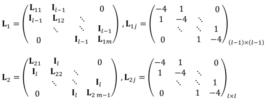
After we know the discrete boundary conditions, the discrete operators can be written as matrices. Consider the laplacian term , it contains the laplacian operators to the horizontal velocity and vertical velocity, called and .

0 0

The discrete Δ _, and Δ _, have been introduced already. Since we

0         0  , 4 1 1 4 0 0 1 1 4   0         0    , 4 1 1 4 0 0 1 1 4

Obviously, is symmetric and negative definite.

The boundary condition term comes from . can be written as

, T_{/2 , where and are}

, , 0, ,0, , ,    , , 0, ,0, , ,       , , , 0,       ,0, , T , , , , , , ,       0,               ,0  , , , , , , , T , , 0, ,0, , ,    , , 0, ,0, , ,       , , , 0,           ,0, , T , , , , , , ,   0,               ,0  , , , , , , , T

To introduce and , refer to [19], let’s see a simple example. Consider the two cells case. There are only four horizontal velocity terms and three vertical

velocity terms, called , , , ,

, , . See fig. 2.

Fig. 2. The two cells case

Consider the discrete divergence term, we know that

∆ ∆ ∆ ∆ 0 

∆ ∆ ∆ ∆ 0 

If we rewrite it to the matrix form, then

12 1 1 0 0 1 1 1 0 0 1 1 0 0 1 ∆ ∆ ∆ 0 0 ∆ ∆ ∆ ∆ 0

Notice that the center matrix is  . Let the left matrix be , so we get the

simple factorization .

Similarly, we also can get the matrix form of and factorize . In the two cells case, can be written as:

∆ _0.5 ∆ _1.5 ∆ _2.5 0 0 ∆ _0.5 ∆ _0.5 ∆ _1.5 ∆ _1.5   1   0 1   1   0 1   1    0 0    1 1   0   0 1

Let the left matrix be and the center matrix be . We can see that

and T.

In general, the matrix form of is

  0 0  , 1 1 0 0 1 1   0 0      ,

The boundary condition term comes from . can be written as:

, , 0, ,0, , ,    , , 0, ,0, , ,       , , , 0,       ,0, ,

T , , , , , , ,       0,             ,0  , , , , ,  , ,

T

If there are not Dirichlet boundary conditions at all. That is, some boundary conditions maybe are Neumann boundary conditions. Let the boundary

∂Ω ∂Ω ∂Ω ∂Ω ∂Ω , and the boundary conditions , , | Ω ,

, , | Ω , ∂ , , | Ω , ∂ , , | Ω are known, where is the

outer normal vector of the boundary.

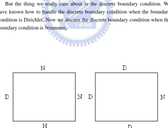
For example, we suppose that ∂Ω , Ω| 0 , ∂Ω ∂Ω\ ∂Ω ,

∂Ω , Ω| X , and ∂Ω ∂Ω\ ∂Ω . In figure 3, it shows the

relationship between the boundary condition type and the place. The boundary

conditions that we know are 0, , , X, , , , 0, ,   , Y, ,

0, , , X, , , , 0, and   , Y, .

But the thing we really care about is the discrete boundary condition. We have known how to handle the discrete boundary condition when the boundary condition is Dirichlet. Now we discuss the discrete boundary condition when the boundary condition is Neumann.

Fig. 3. The left figure represents the boundary condition type of u. The right figure represents the boundary condition type of v.

14

We can use the central difference to approximate , 0, .

1 , 0, 1 ∆ , ,

∆ _.

The discrete boundary condition _, can be approximated by

, , ∆ . · 1 , 0, 1 ∆

But we do not know _, , so this part can be replace by _, , or use the velocity at the time step n and n-1 to approximate _, . That is,

, 2 , ,

This approximation also can be applied when the boundary condition is Dirichlet. So the discrete boundary condition _, can be approximated by

, 2 , , ∆ . · 1 , 0, 1 ∆

Similarly, the other discrete boundary conditions can be written as

, 2 , , ∆ . · 1 , Y, 1 ∆  

, 2 , , ∆ . · X, 1 , 1 ∆  

, 2 , , ∆ · X, 1.5 , 1 ∆

Notice that we are not use the central difference to approximate _, . Because these boundary conditions are approximated by and . After solving , we need to update the discrete boundary conditions. At the next time step, they will be used to compute N .

Although we use the Neumann boundary conditions approximate the boundary velocity, we would rather use the Neumann boundary conditions than use the approximated boundary velocity.

Consider the laplacian operator . For example, we would rather use

0.5 , 0, 1 ∆ than _{, ,} ⁄∆ when we compute the

15

∆ _, , 2 , ,

, , _{0.5 , 0, 1 ∆}

 

        , 3 , , , 0.5 , 0, 1 ∆

Follow this idea, the matrix and the boundary condition also have some change. In this case, the matrix changes to

0 0 0         0  , 0         0  

where and are

3 1 1 3 0 0 1 1 3 1 1 2     if  1 or    3 1 1 4 0 0 1 1 4 1 1 3    for 2 1  4 1 1 4 0 0 1 1 4 1 1 3         The corresponding boundary condition    also has some change. First,  e denote some values         for 1 1  w   1 , 0, 1 ∆   1 , Y, 1 ∆   X, 1.5 , 1 ∆   X, 1 , 1 ∆

16

The corresponding boundary condition    can be written as:

, T_/2 where     _, ,   0,       ,0, ,    _, , 0, ,0, ,       , _, , 0, ,0, T h , , , ,       0,              ,0  , , ,       , T , , 0,  ,0, ,    , , 0, ,0, ,        , , , 0,              ,0, T , , , , , , ,   0,               ,0  , , , , , , , T

Neumann boundary condition also can be used to compute , but we still use the discrete boundary condition and original . If we use the

Neumann boundary condition, the matrix would be changed, the

3

Matrix Factorization Method

3.1 Mathematical formulation

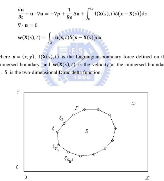
The immersed boundary method was first introduced by Peskin in [7, 8]. Consider the two-dimensional incompressible Navier-Stokes equation with an immersed massless boundary. Let the two-dimensional domain Ω 0, X

0, Y . Let the immersed boundary ∂ , which is a closed curve, as shown in Figure 4. The immersed boundary is tracked by the parametric function s ,

0 s , where is the length of the immersed boundary . The

mathematical formulation is ∂ 1 17 ∆ , δ d   0   , , δ d Ω

where , , , is the Lagrangian boundary force defined on the

immersed boundary, and , is the velocity at the immersed boundary . δ is the two-dimensional Dirac delta function.

Fig. 4. The domain Ω , immersed object , immersed boundary , and the Lagrangian points

18

3.2 Discretization

Similar to the discretization of the incompressible Navier-Stokes equations, we can discretize the mathematical formulation. Refer to [9] , the discretization can be written as:

  ∆ 3 2 1 2 G 2 bc 0 bc  

where and are the discrete regularization operator and the discrete interpolation operator, respectively.

The discrete boundary force f and the discrete boundary velocity are

defined on the Lagrangian markers . We can regard as , where is a

monotone sequence between 0 and , 1 , as shown in figure 4. Let , , we define the distance between each Lagrangian markers ∆ as follows:

∆ | |     for 1 1 

∆

If the arc length of each part is known, we would rather define the arc length ∆ then use distance. Then, we use ∆ define ∆ as follows:

∆ ∆ ∆ ⁄  2

∆ ∆ ∆ ⁄     for 22

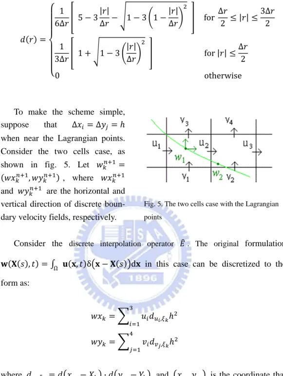
Before we introduce and , the discrete delta function should be introduced first. Here, we use the discrete delta function which was introduced by Roma et al [10].

δ , ·

where the function is

  5 3| | ∆ 1 3 1 | | ∆ 1 6∆ 19        for ∆ 2 | | 3∆ 2   1 1 3 | | ∆ 1 3∆          for | | ∆ 2       0       otherwise       

To make the scheme simple,

suppose that ∆ ∆

when near the Lagrangian points. Consider the two cells case, as shown in fig. 5. Let

, , where

and are the horizontal and vertical direction of discrete boun- dary velocity fields, respectively.

Fig. 5. The two cells case with the Lagrangian points

Consider the discrete interpolation operator . The original formulation

, _Ω , δ d in this case can be discretized to the

form as:

,   ,

where _, · , and , is the coordinate that

is defined. The matrix form of u can be written as: 1, 1 2, 1 3, 1 1, 2 2, 2 3, 2 0 0 1, 1 2, 1 1, 2 2, 2 3, 1 4, 1 3, 2 4, 2 1 2 4 1 2 1 2

20

Similarly, consider the discrete regularization operator . Let , , where and are the horizontal and vertical direction discrete boundary

force, respectively. We can discretize the term , δ d as

follows: 1, 1 1,2 2, 1 2,2 3, 1 3,2 0 0 1,1 1,2 2,1 2,2 3,1 3,2 4,1 4,2 ∆ ∆ 0 0 ∆ ∆ 1 2 1 2

In general case, and can be written as:

, T

where and are

0 0 2,2, 1 2,2, , 1, 1 , 1,   2,2, 1 2,2, 1, , 1 1, ,   0 0   ∆ 0 0 ∆

Notice that for each row of , there are only nine values are nonzero because of the definition of the discrete delta function if we let ∆ .

21

3.3 Matrix factorization method

Put the unknown terms , , and on the left side of the equal sign, and the other terms on the right side. The discretization can be written as:

2 2 3 2 1 2                   0                   Let 2 and ̂ 2 3 2 1 2 1 _{, then} 1 _̂ 1          0          

The matrix factorization method is a projection approach of the immersed boundary method introduced by Taira and Colonius [9]. Similar to the fractional

step method, we have known the facts that and . The

discretization can be rewritten to

1 _̂ 1  1               ₀ 2                    Let 1, , , ̂ , and

. It can be represented by the matrix form as follow:

1 0 1 1 2 0

We know that T, but and do not have the symmetric relation directly. So a transformed forcing function was introduced by Taira and Colonius

22 T T 1 0 1 1 2 0 Let T , λ T, ₁ , and ₂ 1 T: T 1 λ

The fractional step method could be applied here.

T

1

λ T T

1

λ

Here we use N to approximate , there will exist an Nth order error term. T T N N 1 λ N _{λ 2⁄} 0

Let N λ, the matrix factorization method can be written in three steps:

          Solve     

T N _λ T         _{Solve   λ}   N _{λ       Get}   

Since and T N are symmetric and positive definite, conjugate gradient method can be applied to solve and λ. Consider a special case that

∆ ∆ , then . T can be regard as:

       

T ₂

23

4

Numerical Results

4.1 Error estimate of fractional step method

Consider the incompressible Navier-Stokes equations consisting of the momentum and continuity equations. There exists an exact solution that satisfies the Navier-Stokes equations. They are

, , 2 ⁄  

, , 2 ⁄  

, , 2 2 4 ⁄ ⁄ 4

Use this data, we can know the initial and boundary conditions, and compare the numerical solution with the exact solution. We set the computational domain

Ω 0,1 0,1 , the computational time T 1, and the Reynolds number

Re 40.

To check the order of accuracy of the fractional step method, let ∆t 1 400⁄  , 1 800⁄  , 1 1600⁄ , 1 3200⁄  , and  1 6400⁄ , respectively. N 3. Suppose

that ∆ ∆ , and let 40∆t. We define the maximum error by

subtracting the numerical solution from the exact solution and take infinite norms. The order is known by taking on the ratio of the errors. As shown in table. 1, the fractional step method has second-order accuracy in time.

Table 1

The maximum errors from different ∆t

∆t maximum error order 1 400⁄ 1 10⁄ 3.2781e-004 2.47 1 800⁄ 1 20⁄ 5.9040e-005 1.97 1 1600⁄ 1 40⁄ 1.5094e-005 2.01 1 3200⁄ 1 80⁄ 3.7449e-006 1.96 1 6400⁄ 1 160⁄ 9.6555e-007 －

4.2 The flow past a cylinder

Consider a situation that the flow past a cylinder, where the diameter of the cylinder is . The matrix factorization method can be applied here to simulate this situation.

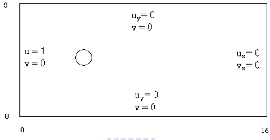
In this test, the computational domain is set by Ω 0,16 0,8 . The Reynolds number Re 100 and 200, respectively. We choose ∆t 1 640⁄

and ∆x ∆y 1 16⁄ . The initial condition is given by | 0 and

| 0. The boundary condition is shown in Fig.6. To construct the cylinder, we put the center of the cylinder at the position 4,4 , and let the diameter

1. Choose the number of the markers 64, then ∆ ⁄ . Notice 64 that ∆ 0.785 .

Fig. 6. The boundary condition and the computational domain

The simulations which the flow past a cylinder at Reynolds number 100 and 200 show the periodic vortex shedding. In figure 7, we can see the periodic vortex shedding in the vorticity contours. The vorticity of the flow is defined as

.

24

There are three quantities, the drag coefficient , lift coefficient , and the Strouhal number . We can use the three quantities to compare this simulation with others. The three quantities are defined as:

2 ⁄  

2 ⁄    

where and are the drag force and lift force, 1 in this simulation, is the frequency of the vortex shedding. and can be obtain in [11], which are

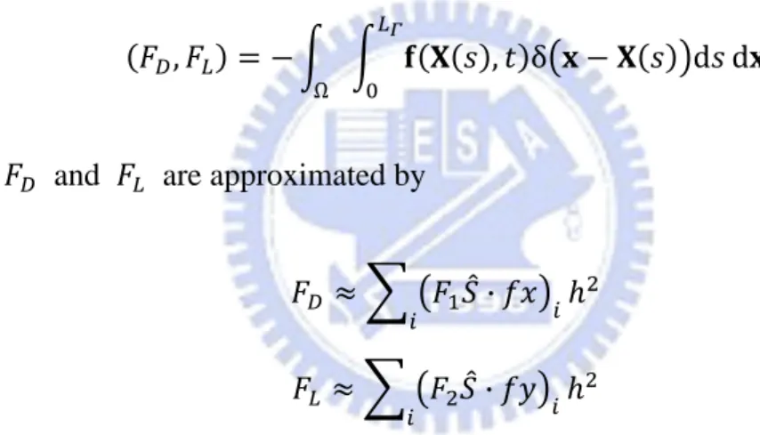
, , δ d d

Ω

and are approximated by

·

·

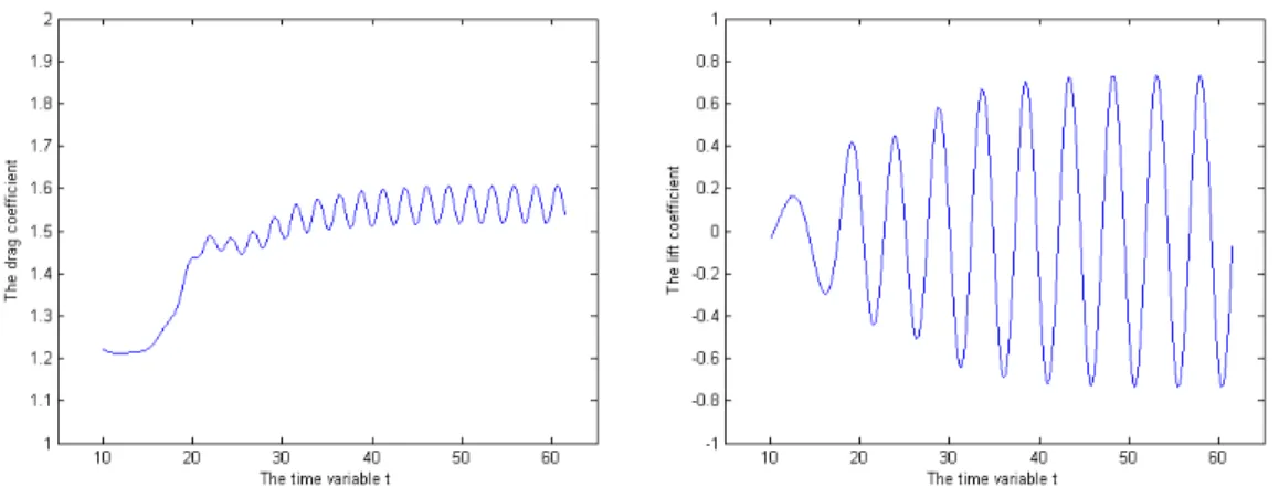
In figure 8 and 9, we can observe the periodic vortex shedding. In table 2 and 3, we compare the three quantities with the previous numerical results which refer to [9, 11, 12, 13, 14, 15] at Reynolds number Re 100 and 200.

25

26

Fig. 9. The time evolution of drag(left) and lift(right) coefficients at Reynolds number Re 200

Table 2

The comparisons of lift and drag coefficients and Strouhal number of Re 100 Present Lai and Peskin[11] Kim et al.[12] Silva et al.[13]

1.64 1.44 1.33 1.39 0.177 0.165 - 0.16 0.40 0.33 0.32 -

Table 3

The comparisons of lift and drag coefficients and Strouhal number of Re 200 Present Taira and Colonius [9] Linnick and Fasel[14] Liu et al[15]

1.56 1.36 1.34 1.31 0.206 0.197 0.197 0.192 0.72 0.69 0.69 0.69

4.3 The flow past two cylinders

In this test, we simulate the flow past two cylinders at the Reynolds number Re 200. Let the diameter of the two cylinders are the same, and set to be

1. Similar to the previous case, we set the computation domain Ω 0,16 0,8 , ∆t 1 640⁄ and ∆x ∆y 1 16⁄ . The initial and boundary conditions are as before, too. To construct the cylinder, we put the centers of this two cylinders at the position 4, 2.5 and 4, 5.5 . We also choose ∆

64

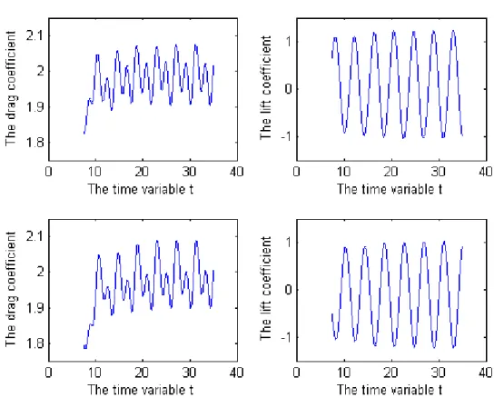
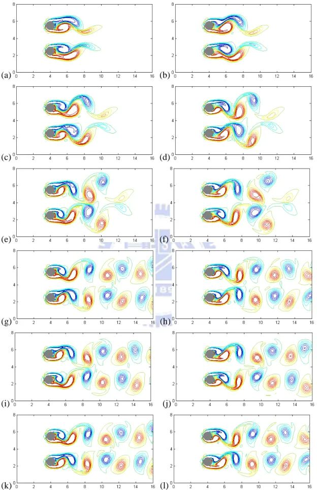
⁄ , so the number of the markers 128. The time evolution of drag and lift coefficients and the vorticity contours are shown in figure 10 and 11. We can observe that the drag coefficients of the two cylinders are similar, and the lift coefficients of the two cylinders are symmetric.

Fig. 10. The time evolution of drag(left) and lift(right) coefficients of the upper(up) and lower (down) cylinders.

(a) (b) (c) (d) (e) (f) (g) (h) (i) (j) (k) (l)

Fig. 11. The vorticity contours when the flow past two cylinders : (a)t=7, (b)t=8, (c)t=9, (d)t=10, (e)t=11, (f)t=12, (g)t=30, (h)t=31, (i)t=32, (j)t=33, (k)t=34, (l)t=35.

4.4 The flow past a wing

Here, we simulate the flow past through a wing of the airplane at the Reynolds number Re 200. We use the same computational domain, mesh, initial condition and boundary conditions as before, but the immersed object. See figure 12, the shape of the immersed object is a airfoil, which is a thin winglike structure. We rotate the wing by an angle, which is 30° here, as shown in figure 13. The periodic vortex shedding also can be observed behind the wing in figure 14.

Fig. 12. The shape of the immersed object

Fig. 13. The placement of the wing

(a) (b)

(c) (d)

(e) (f)

(g) (h)

(i) (j)

Fig. 14. The vorticity contours when the flow past a wing : (a)t=51, (b)t=52, (c)t=53, (d)t=54, (e)t=55, (f)t=56, (g)t=57, (h)t=58, (i)t=59, (j)t=60.

4.5 The flow past an oscillating cylinder

Consider the same simulation as the flow past a cylinder at Reynolds number Re 100, but the cylinder is moving here. We impose the velocity ,

at the boundary as , 0, 0.14 cos 2 , where is the

frequency that the cylinder oscillates. That is, the cylinder oscillates vertical to the stream. Here we choose 2 . The time evolution of drag coefficient and the vorticity contours are shown in figure 15 and 16. Compare with figure 8, we can see that the frequency of the vortex shedding is influenced by the oscillation of the cylinder after the cylinder moves. In table 4, we compare the drag and lift coefficients with the previous numerical results which refer to [17, 18].

Fig. 15. The time evolution of the lift(right) coefficients

Table 4

The comparisons of the lift and drag coefficients

Present Su et al.[17] Hurlbut et al.[18]

1.84 1.70 1.68 1.75 0.97 0.95

(a) (b)

(c) (d)

(e) (f)

(g) (h)

Fig. 16. The vorticity contours when the flow past a oscillating cylinder : (a)t=4.21875, (b)t=4.921875, (c)t=5.625, (d)t=6.328125, (e)t=7.03125, (f)t=7.734325, (g)t=8.4375, (h)t=9.140625.

33

5

Conclusion

In this thesis, we use the matrix factorization method introduced by Taira and Colonius [9] to simulate the flow past as immersed object. In the numerical result, we see that this method can handle the immersed object with complex shape, and which the immersed object is moving, even the two or more objects. It is useful in the engineering applications. In Section 4.4, we simulate the situation when the flow past a wing. The flow produces vortex shedding behind the wing.

Here we suppose that the mesh widths of each cell are the same, that is, we let ∆ ∆ for all , . In fact, the matrix factorization method can use the different grid size of each cell. If the higher accuracy is desired, the grid size near the immersed object has to be small. We can adapt the code to handle the different mesh widths, to improve the accuracy.

34

References

[1] A.J. Chorin, “Numerical solution of the Navier–Stokes equations.” Math. Comput. Vol. 22, pp. 745–762, 1968. [2] J. Kim, P. Moin, “Application of a fractional-step method to incompressible Navier–Stokes equations.” J. Comput. Phys.

Vol. 59, pp. 308–323, 1985.

[3] J.B. Perot, “An analysis of the fractional step method.” J. Comput. Phys. 108 51–58, 1993.

[4] R. Codina, “Pressure stability in fractional step finite element methods for incompressible flows.” J. Comput. Phys. Vol. 170, pp. 112–140, 2001.

[5] F.H. Harlow, J.E. Welsh, “Numerical calculation of time-dependent viscous incompressible flow of fluid with a free surface.” Phys. Fluids. Vol. 8, pp. 2181-2189, 1965.

[6] D.L. Brown, R. Cortez, M.L. Minion, “Accurate projection methods for the incompressible Navier–Stokes equations.” J. Comput. Phys. Vol. 168, pp. 464–499, 2001.

[7] C.S. Peskin, “Flow patterns around heart valves: a numerical method.” J. Comput. Phys. Vol. 10, pp. 252–271, 1972. [8] C.S. Peskin, “The immersed boundary method”. Acta Numer. Vol. 11, pp. 479-517, 2002.

[9] K. Taira, T. Colonius, “The immersed boundary method: A projection approach.” J. Comput. Phys. Vol. 225, pp. 2118-2137, 2007.

[10] A.M. Roma, C.S. Peskin, M.J. Berger, “An adaptive version of the immersed boundary method.” J. Comput. Phys. Vol. 153, pp. 509–534, 1999.

[11] M. Lai, C.S. Peskin, “An immersed boundary method with formal second-order accuracy and reduced numerical viscosity.” J. Comput. Phys. Vol. 160, pp. 705–719, 2000.

[12] J. Kim, D. Kim, H. Choi, “An immersed-boundary finite-volume method for simulations of flow in complex geometries.” J. Comput. Phys. Vol. 171, pp. 132-150, 2001.

[13] A. L. F. Lima E Silva, A. Silveira-Neto, J. J. R. Damasceno, “Numerical simulation of two-dimensional flows over a circular cylinder using the immersed boundary method.” J. Comput. Phys. Vol. 189, pp. 351-370, 2003.

[14] M.N. Linnick, H.F. Fasel, “A high-order immersed interface method for simulating unsteady incompressible flows on irregular domains.” J. Comput. Phys. Vol. 204, pp. 157–192, 2005.

[15] C. Liu, X. Zheng, C.H. Sung, “Preconditioned multigrid methods for unsteady incompressible flows.” J. Comput. Phys. Vol. 39, pp. 35–57, 1998. 1

[16] R. Témam, “Sur l’approximation de la solution des équations de Navier–Stokes par la méthode des pas fractionnaires.” Arch. Rat. Mech. Anal. Vol. 32 (2), pp. 135–153, 1969.

[17] S. Su, M. Lai, C. Lin, “An immersed boundary technique or simulating complex flows with rigid boundary.” Comput. Fluids. Vol. 36, pp. 313-324, 2007.

[18] S.E. Hurlbut, M.L. Spaulding, F.M. White, “Numerical Solution for Laminar Two Dimensional Flow About a Cylinder Oscillating in a Uniform Stream”, Trans ASME, J. Fluids Eng. Vol. 104, pp. 214-221, 1982.

[19] W. Chang, F. Giraldo, B. Perot, “Analysis of an exact fractional step method.” J. Comput. Phys. Vol. 180, pp. 183–199, 2002.