利用統計方法提升行動裝置硬體指紋之準確率

1

利用統計方法提升行動裝置硬體指紋之準確率

Improve Mobile Device Fingerprinting Accuracy by

Fusion of Statistical Methods

研 究 生：王鼎鈞 Student：Ting-Chun Wang

指導教授：謝續平 博士 Advisor：Dr. Shiuhpyng Shieh

國 立 交 通 大 學

資 訊 科 學 與 工 程 研 究 所

碩 士 論 文

A Thesis

Submitted to Institute of Network Engineering

College of Computer Science

National Chiao Tung University

in partial Fulfillment of the Requirements

for the Degree of

Master

in

Computer Science

July 2008

Hsinchu, Taiwan, Republic of China

中華民國九十七年七月

i

利用統計方法提升行動裝置硬體指紋之準確率

研究生：王鼎鈞 指導教授：謝續平

國立交通大學 資訊科學與工程研究所

摘 要

硬體裝置識別是網路安全中非常重要的議題。攻擊者可能使用竊

取或是假造的身分去進行非法的行為或攻擊，這使得蒐集證據變得

更為困難。之前的研究中提出一個稱為遠端硬體裝置指紋的技術，

利用從裝置送出的 TCP 封包中取出時間戳記內包含的時間訊息計算

出該裝置的時間歪斜誤差(clock skew error)來做為該裝置的硬體

指紋。但時間歪斜會因為硬體的特性和網路的傳輸延遲而變的不穩

定，特別是對行動裝置來說這個不穩定更為的明顯。在此篇論文中

我們利用統計的模型來提升行動裝置硬體指紋的準確率。並且根據

這個行動裝置硬體指紋的技術提出了一個偽造身分檢測的方法。實

驗的結果顯示我們提出的方法可以有效的偵測出偽造身分攻擊，並

且相較於之前的研究有著更高的準確度。

ii

Improve Mobile Device Fingerprinting Accuracy by

Fusion of Statistical Methods

Student: Ting-Chun Wang Advisor: Shiuhpyng Shieh

Department of Computer Science

National Chiao Tung University

Abstract

Device identification is one of the most important issues to Internet

security. An adversary can take illegal actions with stolen or forged

identity that makes evidence collecting to be very difficult. Previous

work introduces an intuitive method that identifies a device by its clock

skew. Unfortunately, the clock skew of a device is instable over time in

the mobile environment due to the characteristics of the hardware and

the instability of network latency. In this paper we adapt a statistical

method inspired by EWMA model that characterizes the tendency of

clock skew changes to improve the accuracy of mobile device

fingerprinting. We also propose a device identity spoofing detection

scheme based on the improved mobile device fingerprinting technique.

The experiment result shows that the proposed scheme effectively

detects identity spoofing attacks with higher accuracy compared to

prior works.

iii

致謝

iv

Table of Contents

1. Introduction... 1

2. Related Work ... 3

3. Clock Skew Based fingerprinting technique for mobile devices... 5

3.1. Kohno’s remote physical device fingerprinting technique ... 5

3.2. Instability of Mobile Device’s Clock Skew ... 7

3.3. The Proposed Mobile Device Fingerprinting Technique ... 11

3.4. Proposed device identity spoofing detection scheme... 16

4. Experiments and Results... 23

4.1. Required packet number to estimate a clock skew ... 23

4.2. Required Profile Sample Size ... 24

4.3. Accuracy evaluation of the proposed device identity spoofing detection scheme 25 4.3.1. Environment and Settings ... 26

4.3.2. Error rate evaluation... 26

5. Conclusion ... 29

v

List of Figures

Figure 3.1: Typical Frequency vs Temperature Curve for various angle of AT-cut crystals. ... 9

Figure 3.2: The clock skew error and CPU temperature change over time of a ASUS W7J Laptop ... 10

Figure 3.3: Incremental Learning Example of 2 minute retraining interval ... 14

Figure 3.4: The relation of L and False Accept Rate and False Reject Rate ... 16

Figure 3.5: Flow chart of the training phase... 17

Figure 3.6: The procedures of Device Profile Building Module ... 18

Figure 3.7: Flow chart of testing phase and retraining phase ... 20

Figure 3.8: The procedures of clock skew verification module ... 21

Figure 3.9: The procedures of updating module... 22

Figure 4.1 Segment size n versus average difference. ... 23

vi

List of Tables

Table 3.1: Electrical Specification – maximum limitation values ... 8 Table 4.1: Error rate comparison ... 27

1

1. Introduction

With the rapid evolution of automation services and environment information

monitoring applications, the information is directly acquired from the devices

without human intervention. Take automatic fire alarm system as an example, the

temperature information is sampled by temperature sensor devices that placed in

the monitored area. Once a sensor device found that the temperature is over an

unusual level or a fixed threshold, there might be a fire accident in the monitored

area. Then it may issue an alarm to evacuate all the personnel or automatically

report to the fire department. Unfortunately, these devices are not been properly

protected, attackers may directly replace one or some of the sensor devices to

crash the system. Verifying the device‟s identity has become more and more

important.

The main idea of remote device fingerprinting is utilizing the hardware

specification or firmware behavior to represent the identity of a physical device .

There are two roles in remote device fingerprinting: the fingerprinter and the

fingerprintee. The fingerprinter must acquire some information from the

fingerprintee to verify the identity of the fingerprintee. The two devices must be

connected to each other to exchange information. Since most of the modern

devices have the ability to access to the Internet, they can communicate with each

other through well know Internet protocols such as TCP and UDP.

There are three main classes of remote physical device fingerprinting

techniques: passive, active, and semipassive. The passive fingerprinting technique

2

fingerprintee and the fingerprintee did not aware that it has been fingerprinted.

The active fingerprinting technique is that the fingerprinter must issue a

fingerprinting request to ask the fingerprintee to present the information for

fingerprinting. The third class of fingerprinting technique is that after the

fingerprintee initiates a connection, the fingerprinter can interact with the

fingerprintee over that connection. There are both advantage and disadvantage of

each class. For example, the advantage of passive fingerprinting is that the

fingerprinter is completely undetectable to the fingerprintee. The disadvantage of

passive fingerprinting is that if the fingerprintee is behind a NAT or firewall, the

3

2. Related Work

There are several techniques that had been proposed to fingerprint a physical

device. These techniques can be categorized into three categories. The first

category takes the device‟s unique identifier as its fingerprint. For example, the

MAC address is suitable for fingerprinting a network interface card. However,

these identifiers can be easily modified or forged therefore this type of

fingerprinting techniques can only apply to lower security concern applications.

The second category utilizes the firmware behavior to fingerprint a certain

physical device. The main reason that each device performs different behavior is

that some of the detailed algorithms are not clearly defined in the protocol

standards. The device manufacturer can design their own ones therefore leave the

trace to classify them from other manufacturers. Franklin et al. [1] proposed a

passive fingerprinting technique that classifies the wireless network interfaces

through their behavior when they are applying active scanning. According to the

same concept, Corbett [2] proposed another scheme that classifies the wireless

network device by observing their rate switching algorithms. The drawback of this

kind of fingerprinting techniques is that they can only classify devices on model

level, that is, knowing a certain device is belongs to which model of some

manufacturer. If there are two devices that happens to be exactly same model or

same manufacturer, this type of fingerprinting techniques will not be able to tell

them apart.

The last category of device fingerprinting techniques is based on hardware

specifications of the fingerprinted device. It gathers the hardware information

4

together to form a information matrix to represent a device‟s fingerprint. It has

been widely deployed on many software registration or activation processes.

Microsoft Windows utilize this type of fingerprinting technique in its activation

process to avoid two or more machines use the same activation number.

Clock skew is another hardware specification that can be used to fingerprint a

physical device. Every device has its own clock, and the quassation frequency of

the oscillator in every device is slightly different thus can be used to differentiate

two given devices. Based on this characteristic Kohno et al. [3]proposed a remote

physical device fingerprinting technique that estimates the clock difference of the

fingerprinter‟s system clock and the fingerprintee‟s TCP timestamp. The

experiment result of this technique is impressive, but the clock is not always the

same especially in mobile environment. In this paper we based on Kohno‟s work

5

3. Clock Skew Based fingerprinting

technique for mobile devices

In this chapter, our mobile device fingerprinting technique will be presented

which is inspired by Kohno‟s remote physical device fingerprinting technique [3]

and Exponentially Weighted Moving Average Model [4]. We will first give a brief

introduction on Kohno‟s work, and then we will explain why Kohno‟s work will

not be able to apply to fingerprint a mobile device. Finally, we will give our

proposed mobile device fingerprinting technique.

3.1. Kohno’s remote physical device fingerprinting technique

physical identity from its timing information. They estimated the machine‟s clock

skew by examining the timestamps embedded in the TCP and ICMP packets sent

by that machine.

Kohno formalized the timing relation between the fingerprinter ‟s clock and

the fingerprintee‟s TCP timestamp value as follow: Let T be a set of data that

observed by the fingerprinter and let ti be the time in seconds at which the

fingerprinter received the ith packet in T and let Ti be the timestamp contained

within the ith packet. Define

𝑥𝑖 = 𝑡𝑖− 𝑡1

6

𝑤_𝑖 = 𝑣_𝑖 Hz 𝑦𝑖 = 𝑤𝑖 − 𝑥𝑖

𝑂_𝑇 = 𝑥_𝑖 , 𝑦_𝑖 ∶ 𝑖 ∈ 1 … … 𝑇

The unit for 𝑤_𝑖 is seconds, 𝑦_𝑖 is the observed offset of the ith packet. Hz is the intended frequency, the inverse of its resolution; e.g., a clock with 10 ms

granularity is designed to run at 100 Hz. 𝑂𝑇 is the offset-set corresponding to the

observed data set 𝑇.

Assuming that the fingerprinter‟s clock is the accurate and that the t values

represent true time, and there is no delay between when the fingerprintee

generates the ith packet and when the fingerprinter capture the ith packet, then

𝑦_𝑖 = off 𝑥_𝑖+ 𝑡₁ . The first derivative of y, which is the slope of the points in 𝑂_𝑇, is the clock skew s of the fingerprintee. Since we cannot generally make these

assumptions, we can only approximate s from the observed data set.

There are many algorithms for calculate the linear regression from a give

set of points. The most common one is simple least-squares linear regression

algorithm [18], but both Paxson [6] and Moon [5] noted that simple least-squares

linear regression algorithm will be insufficient for data that contains variable

network delay. Consequently, Kohno borrow the linear programming solution

from Moon et al. [5][8] to approximate the slope of y, i.e. the clock skew of the

fingerprintee.

The linear programming calculates the equation of a line 𝑦 = 𝛼𝑥 + 𝛽 that upper-bounds all the points in 𝑂_𝑇. That is, for all 𝑖 ∈ 1 … … 𝑇 ,

7

The linear programming solution then minimizes the average vertical distance of

al the points in 𝑂_𝑇 from the line. That is, minimizes the objective function 1

𝑇 ∙ 𝛼 ∙ 𝑥𝑖+ 𝛽 − 𝑦𝑖 𝑇

𝑖=1

Moon et al. [5] noted that instead of solving this objective function by standard

linear programming techniques, there exist techniques that solve the linear

programming problems in two variables in linear time. Kohno apply Moon‟s

technique in all his experiment.

Kohno found that a particular device‟s clock skew deviates very little over

time, around 1-2 parts per million (ppm), but that there was a significant

difference between the clock skews (up to 50 ppm) of different devices, even if

they are identical models. This allows the clock skew of a device to act as a

fingerprint. Assuming a stability of 1 ppm, 4-6 bits of information can be

extracted to act as a device‟s identity.

3.2. Instability of Mobile Device’s Clock Skew

Although the experiment result of Kohno‟s work shows that the clock skew is

very stable over time, but this result cannot apply to estimating the clock skew of

a mobile device. There are two source of 變因 in clock skew estimation, one is

temperature and the other one is network transmission delay. We will describe in

detail as follow.

Impact of Temperature

8

1990s [9][10] by the NTP community. Kohno do mention that temperature might affect the clock skew of a device but he leave it as a future work that would help

provide greater insights into the efficacy of his technique.

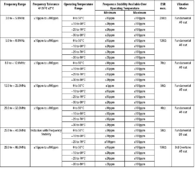
Table 3.1: Electrical Specification – maximum limitation values

Table 3.1 shows the electrical specification of the clock skew error of a AT-cut

crystal that is common for PCs under different working temperature and figure 3.1

graphically illustrate the relation of working temperature and frequency [11]. The

9

changes, which is way over Kohno‟s assumption that the clock skew of a device

has a stability of 1ppm. That is because Kohno‟s experiment is made on general

purpose PCs that the temperature is relatively stable over time. Murdoch [12]

proposed an attack model on anonymity systems that support hidden services, e.g.

Tor [13] , based on the temperature impact on clock skew.

Figure 3.1: Typical Frequency vs Temperature Curve for various angle of AT-cut

crystals.

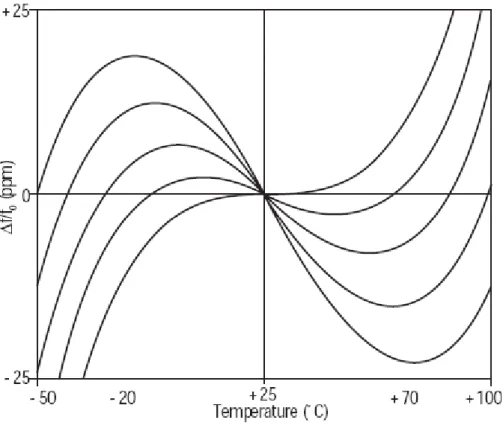
We made a similar experiment as Murdoch did but record the CPU‟s

temperature of a laptop instead of record the temperature in the room. The model

of the laptop is ASUS W7J. The temperature was record directly from the system

utility mbmon [14]. The TCP packets sent from the laptop was captured on the

10

minutes. Figure 3.2 shows the experiment result that the device‟s clock skew is

highly related with the temperature changes.

Figure 3.2: The clock skew error and CPU temperature change over time of a

ASUS W7J Laptop

The working environment of a mobile device changes rapidly so that the

impact of temperature on device‟s clock skew is more noticeable. The lifetime

with only battery power is a major consideration of a mobile device that leads to

many modern power saving techniques being proposed. For example, many

modern processors will automatically turn into sleeping mode when it is in idle

state. Some processors will switch to lower frequency when the working load is

not very high or the battery power is running out. Some laptop manufacturer will

11

range. All the power saving techniques mentioned above would result in dramatic

vary of the device‟s temperature therefore makes the device‟s clock skew to be

instable.

Impact of Network Topology and Transmission Delays

Kohno‟s method is based on the timing information of the fingerprinter‟s

system clock and the fingerprintee‟s TCP timestamps. If the transmission delay is

stable over time, this delay will be part of the 𝛽 value in the line equation. But once again, we cannot generally assume that the delay is constant, especially for

mobile devices. That is because the mobile devices could send out some packets

while moving. Another situation is that the mobile device may roam from one

Access Point to another or one network infrastructure to another, e.g. from Wifi to

WiMax. The different network topology results in different transmission path of

each packet. These differences will reflect in the transmission delay. The i nstable

transmission delay will affect both 𝛼 and 𝛽 value of the line equation. That is, affect the estimate clock skew of the mobile device.

3.3. The Proposed Mobile Device Fingerprinting Technique

We have described the reasons that why the clock skews of mobile devices

will not remain stable over ti me. Duo to the instability of clock skews, some

applications that based on the device fingerprinting technique will fail to work

anymore. For example, the application that utilizes the clock skew based device

fingerprinting technique to track a mobile device will not be able to keep tracking

the target device if the clock skew of the device changes when it moves from

12

two or more devices in the same location that their clock skews are close.

Fortunately, the major factor that affects the clock skew is the temperature

changes, and it is smooth over time. As the experiment results shows in Fig.2, the

temperature of a device‟s CPU will not dramatically change. The largest

temperature difference is between minute 5 and minute 10 that the temperature

raised about 2.6 degrees. The resulting clock skew difference is about 2.2 ppm.

And another important finding in the experiment is that the temperature tends to

keep increase or decrease over a period of time. As shown in Fig.2, the

temperature keep rising between the first 20 minutes and keep falling between

minute 85 to minute 120. We apply statistical model called Exponentially

Weighted Moving Average that can adapt to small changes to improve the

accuracy of device fingerprinting.

Expone ntially Weighted Moving Average Model

We took clock skew as a feature value and used statistical method

Exponentially Weighted Moving Average (EWMA) to calculate historical

averages for feature changes. This method allows us to smooth out fluctuations in

the clock skew variations.

Let x(i) represent the clock skew of a target device‟s feature Z that observed

on time i. Using EWMA we calculate the moving average z(p) as [15]:

𝑧 𝑝 = λ ∙ 𝑥 𝑝 + 1 − λ ∙ 𝑧 𝑝 − 1 , 0 < λ < 1 The average and standard deviation of 𝑧 𝑝 are:

13

σ_𝑧2 _{= σ} 𝑥 2 _∙ λ

1 − λ

Where σ_𝑥 and 𝑢_𝑥 are calculated during the training phase. Lower and upper bound limits are:

Lower Bound: 𝐿𝐶𝐿_𝑧 = 𝑢_𝑧 − 𝐿 ∙ σ_𝑧 Upper Bound: 𝑈𝐶𝐿𝑧 = 𝑢𝑧 + 𝐿 ∙ σ𝑧

The L value is the tolerance coefficients that can be tuned to adapt the current

environment. If 𝑧 𝑝 falls outside [𝐿𝐶𝐿_𝑧 ,𝑈𝐶𝐿_𝑧 ] then the current average is far from the training average, and the case is considered to be two different

fingerprintee, If we wish the system to be strict, we can set L to a smaller value.

On the contrary, if we wish the system to be a little bit looser, we can set L to a

larger value.

Incre mental Learning

After the the EWMA model of the fingerprintee is trained and put into test,

we adapt incremental learning in order to let the EWMA model precisely reflect

the current characteristic of the fingerprintee in real time. As compare to classical

modeling, in which testing phase starts after that training phase is completed, our

model will be retrained and the parameters will be updated after each test.

The concept of the incremental learning is similar to k-fold cross-validation

[16] which is widely applied in training and testing models. The difference is that

14

cross-validation, the provided data is partitioned into k subsamples, and each

subsample is used once as the test data, while the rest of sample is used as training

data. The k results are the averaged to produce a single estimation. In incremental

learning, the weighted moving average is calculated over historical training data,

and the test data is always the „current‟ sampled data that will become the training

data in the next interval.

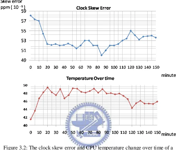
Figure 3.3 illustrates an example of incremental learning after each testing.

Each time the timing information of the target device is received; we calculate its

clock skew base on Kohno‟s fingerprinting technique and test by the previous

training data. If the clock skew falls outside the control limits [𝐿𝐶𝐿_𝑧 ,𝑈𝐶𝐿_𝑧 ], the fingerprinter issues an alert that there might be something wrong with this device.

If the clock skew falls within the control limits, the fingerprinter take the current

clock skew value and the previous training data together as the new training data

and update the EWMA model for next testing period. In other words, Testingi is

performed against CLi (Control Limits), which is taken into effect at Trainingi+1.

Figure 3.3: Incremental Learning Example of 2 minute retraining interval

The incremental learning keeps the EWMA model precisely represents the

characteristic of the target device.

Tuning of Statistical Parameters

Training₀ Training₁ Training₂ Training_i Testing₀ Testing₁ Testing_i-1

Training_i+1 Testing_i time of testing . . . . . . . . . . 0 1 2 i (i+1) CL₀ CL₁ CL_i-1 CL_i

15

The EWMA model and parameters of the target fingerprintee need to be

fine-tuned before they are put into work. Parameters and initial values in EWMA

model, tolerance coefficients need to be carefully determine during the training

period. Ming [17] proved that exponentially weighted moving average filters are

identical to first-order low-pass filters. Thus, we have used low-pass filters

formulas to determine the appropriate value for λ parameter in EWMA formulas.

For each device, we run a (long) single training-test with an initial value like

λ0 = 0.1 and calculate the clock skew value every 𝑇𝑠 time. After that the

training period elapses, we measure average frequency of false alarms for the rest

of dataset, to be named 𝑓_𝑐. This parameter is equivalent to Turn-Over Frequency of a low-pass filter. The time-constant parameter of such a filter is calculated as:

𝑇_𝑓 = 1 2π ∙ 𝑓_𝑐 Then the λ parameter is parameter is [17]:

λ = 𝑇𝑠 𝑇𝑓 + 𝑇𝑠

Since the physical characteristic of each device‟s clock is different, we cannot

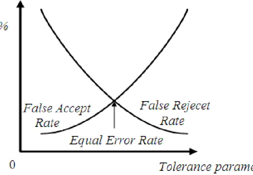
apply normal distribution model to determinate the tolerance value L. We first

define the False Reject and the False Accept that will be used to determinate the L

parameter. False Reject means that the clock skew of the target device is rejected by

the EWMA filter, and False Accept means that the clock skew or other device is

accepted by the EWMA filter. We take the data in the training phase to run the test

by first setting L to be 0.1 and calculate the False Reject Rate. We repeat the testing

and each time the L value is increased by 0.1. In order to calculate the False Accept

16

testing and calculate the False Accept Rate of each L value. The False Reject Rate

will decrease as L increase and the False Accept Rate will increase as L increase.

The two rates will eventually reach at the same value, which we called the Equal

Error Rate. Figure 3.4 illustrate the relation of L and False Accept Rate and False

Reject Rate. Then this L value is suitable for this device.

Figure 3.4: The relation of L and False Accept Rate and False Reject Rate

3.4. Proposed device identity spoofing detection scheme

Now we are going to show that how our mobile device fingerprinting

technique can be apply to applications such as detecting device identity spoofing

attack. There are three phases in our detection scheme: the training phase, the

testing phase, and the retraining phase. The training phase builds a profile that

contains an initial EWMA model and testing parameters for a device that will be

detected later on. After collecting sufficient data, we calculate the device‟s clock

17

limit, the model will be updated with both previous and current clock skews in the

retraining phase.

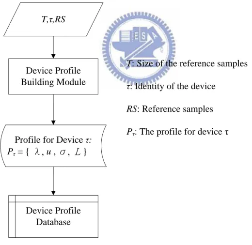
In the training phase, we build a profile that contains an EWMA model and

control limits parameters for the target device. First, a number of reference

samples of the device‟s clock skew are collected. After collecting sufficient number of sample data, the parameters for the EWMA model will be generated by

the methods we have described above. The model will be more accurate if the

sample data is larger. Figure 3.5 depicts the training phase process and the

procedures of device profile building module are showed in Figure 3.6.

T,τ,RS

Device Profile Building Module

Profile for Device τ:

Pτ = { λ, u , σ, L }

Device Profile Database

T: Size of the reference samples τ: Identity of the device

RS: Reference samples Pτ: The profile for device τ

Figure 3.5: Flow chart of the training phase

18

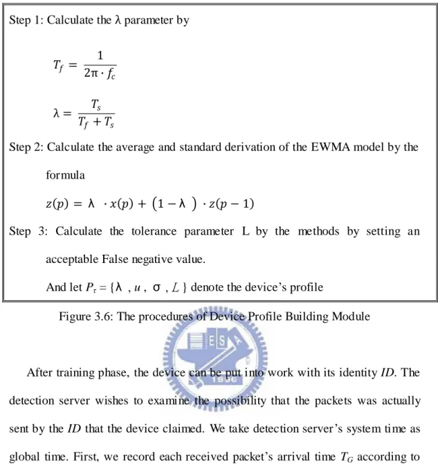
Step 1: Calculate the λ parameter by

𝑇𝑓 =

1 2π ∙ 𝑓_𝑐 λ = _𝑇 𝑇𝑠

𝑓 + 𝑇𝑠

Step 2: Calculate the average and standard derivation of the EWMA model by the

formula

𝑧 𝑝 = λ ∙ 𝑥 𝑝 + 1 − λ ∙ 𝑧 𝑝 − 1

Step 3: Calculate the tolerance parameter L by the methods by setting an

acceptable False negative value.

And let Pτ = {λ , u , σ , L } denote the device‟s profile

Figure 3.6: The procedures of Device Profile Building Module

After training phase, the device can be put into work with its identity ID. The

detection server wishes to examine the possibility that the packets was actually

sent by the ID that the device claimed. We take detection server‟s system time as

global time. First, we record each received packet‟s arrival time TG according to

global time. After receiving a batch of packets, we extract the timing information

TD within each packet‟s TCP header. At this time, we have

𝑇𝐺 = 𝑡1, 𝑡2, ⋯ , 𝑡𝑛

𝑇_𝐷= 𝑡𝑑₁,𝑡𝑑₂, ⋯ , 𝑡𝑑_𝑛

Next, we put these timing information data into the clock skew calculation module

that apply Kohno‟s linear programming algorithm that outputs the clock skew SID.

19

EWMA model and control limits parameters. The lower bound and upper bond

control limits are produced as follows:

𝐿𝐶𝐿_𝐼𝐷 = 𝑢_𝐼𝐷 − 𝐿_𝐼𝐷 ∙ σ_𝐼𝐷 𝑈𝐶𝐿𝐼𝐷 = 𝑢𝐼𝐷 + 𝐿𝐼𝐷∙ σ𝐼𝐷

where 𝑢_𝐼𝐷 and σ_𝐼𝐷 are the average and standard deviation of the ID‟s clock skew, and 𝐿_𝐼𝐷 is the tolerance coefficient. Then we use these lower and upper control limits to test if the SID matches the stored average if

𝐿𝐶𝐿𝐼𝐷 < 𝑆𝐼𝐷 < 𝑈𝐶𝐿𝐼𝐷

The testing phase is showed in Figure 3.7 and the procedures of clock skew

20 ID, TD , TG Device Profile Database Clock skew Verification Module LCLID < SID < UCLID PID = {λ, u , σ, L} Updating Module Pass Fail ID SID Yes No PID

· ID: Claimed identity of the device

· TG: Timing information of global time

· TD: Timing information of the device ID

· PID: The Profile for device ID

· LCLID: Lower control limit for device ID

· UCLID: Upper control limit for device ID

· SID : Calculated Clock Skew of device ID

21

Clock Skew Verification Module:

Step 1: Transform 𝑇_𝐺 and 𝑇_𝐷 into the form of Kohno‟s formula. 𝑥_𝑖 = 𝑡_𝑖− 𝑡₁

𝑣_𝑖 = 𝑡𝑑_𝑖− 𝑡𝑑₁ 𝑤_𝑖 = 𝑣_𝑖 Hz 𝑦_𝑖 = 𝑤_𝑖− 𝑥_𝑖

𝑂_𝑇 = 𝑥_𝑖 ,𝑦_𝑖 ∶ 𝑖 ∈ 1 … … 𝑇_𝐺 Step 2: Solve the objective function

1

𝑇𝐺 ∙ 𝑆𝐼𝐷 ∙ 𝑥𝑖+ 𝛽 − 𝑦𝑖

𝑇𝐺

𝑖=1

to get the estimated clock skew 𝑆_𝐼𝐷

Step 3: Calculate 𝐿𝐶𝐿_𝐼𝐷 and 𝑈𝐶𝐿_𝐼𝐷 from the parameters in device profile 𝑃_𝐼𝐷 𝐿𝐶𝐿_𝐼𝐷 = 𝑢_𝐼𝐷 − 𝐿_𝐼𝐷 ∙ σ_𝐼𝐷

𝑈𝐶𝐿𝐼𝐷 = 𝑢𝐼𝐷 + 𝐿𝐼𝐷 ∙ σ𝐼𝐷

Figure 3.8: The procedures of clock skew verification module

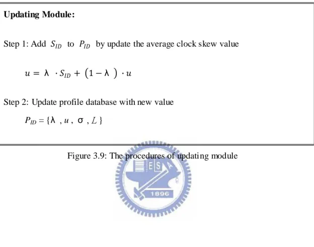
If the calculated clock skew 𝑆_𝐼𝐷 falls within [𝐿𝐶𝐿_𝐼𝐷 ,𝑈𝐶𝐿_𝐼𝐷 ], the system that will enter the retraining phase. In the retraining phase, the verified clock skew

𝑆𝐼𝐷 is added to the EWMA model by the updating module in the retraining phase.

Although our model takes all the sample data to calculate the average clock skew,

but the parameter λ in the EWMA model make the newer data weighted more than the old ones in the average value. If there are n sample data, the ith data weighted

22

the device. Then the updated profile is saved back to device profile database.

The retraining phase processes is showed in Figure 3.7 and the procedures of

updating module are showed in Figure 3.9.

Updating Module:

Step 1: Add 𝑆_𝐼𝐷 to 𝑃_𝐼𝐷 by update the average clock skew value 𝑢 = λ ∙ 𝑆_𝐼𝐷 + 1 − λ ∙ 𝑢

Step 2: Update profile database with new value

PID = {λ , u , σ , L }

23

4. Experiments and Results

To evaluate our proposed technique, we make an experiment to implement the

described device identity spoofing detection scheme in chapter 3. In this chapter, 3

experiments will be presented. We will first depict the environment and settings and

data collection of each experiment, and then we will show up the experimental

results.

4.1. Required packet number to estimate a clock skew

Before we start to evaluate our scheme, we need to know how many timestamps

(or packets) we have to acquire to estimate a device‟s clock skew with an acceptable

granularity. We capture all the packets that sent from the device for a longtime (2

days in our experiment) and use all of them to estimate the “target” clock skew.

Then we divide all the data into contiguous non-overlapping segments of size n and

estimate the clock skew of each segment. For each value of n, we calculate the

average difference of each clock skew and the target clock skew.

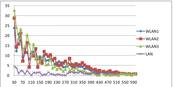
Figure 4.1 Segment size n versus average difference.

0 5 10 15 20 25 30 35 30 70 110 150 190 230 270 310 350 390 430 470 510 550 590 WLAN1 WLAN2 WLAN3 LAN

24

Figure 4.1 shows the average difference related to the segment size n. For the

LAN device, the clock skew is relatively stable compare to the other three WLAN

devices. It shows that only 60 packets are required to estimate a clock skew on a

LAN device.

For the three WLAN devices, the average difference remains very high (over 5

ppm) until segment size n reaches 370. The reason is that the network latency of the

WLAN environment is relatively instable compare to LAN. The experiment result

shows that it takes over 500 packets to estimate an acceptable clock skew for a

WLAN device.

4.2. Required Profile Sample Size

Now we know the required numbers of packet to estimate an acceptable clock

skew, we now moving on to figure out how many clock skew samples required to

build a device profile that can really characterize the tendency of the clock skew

change.

The data set is the same as the experiment described in section 4.1. We calculate

the clock skew of each device every 500 packets. The first m estimated clock skews

are used to build the device profile with our proposed scheme and the rest of the

clock skews are used to test the device profile. If the clock skew were rejected in the

testing phase, we count it as a false rejection. For each value of m, we divided false

rejection counts by the total test time to get the false-reject rate. Figure 4.2 shows

the false-reject rate related to the profile sample size m. For the LAN device, the

25

Figure 4.2 False-Reject Rate versus profile sample size

The false-reject rate of the three WLAN devices, on the other hand, remains over

10% when the profile sample size becomes 20. The false-reject rate of the 4 device

dropped below 3% when the profile sample size over 50. Therefore, if we want to

build a profile that tightly characterize the tendency of the clock skew changes; the

required profile sample size should be over 50.

4.3. Accuracy evaluation of the proposed device identity spoofing

detection scheme

After knowing how many packets to estimate an acceptable clock skew and the

required sample size to build an accurate device profile, we are going to evaluate the

accuracy of our proposed device identity spoofing detection scheme.

0 3 6 9 12 15 18 21 24 27 30 33 36 39 0 10 20 30 40 50 60 WLAN1 WLAN2 WLAN3 LAN

26

4.3.1. Environment and Settings

There are three roles in our experiment, the detection server, the legitimate

devices and the attacker. The detection server is located at the backend of the

network that can retrieve all the packets sent by every legitimate devices and

attacker. After the device profile is build, the legitimate devices are going to perform

their normal work. The attacker, on the other hand, will deploy identity spoofing

attack that randomly sends packets with one of the legitimate identities.

There are 1 detection server, 11 legitimate devices and 1 attacker in our

experiment. From the experiment result of the experiment in section 4.1 and 4.2, we

estimate the clock skew every 500 packets and build the device profile with 50

samples. We run the experiment for two days to evaluate the accuracy of the

proposed scheme.

4.3.2. Error rate evaluation

In order to evaluate the error rate of the proposed scheme, we first defi ne the

error situation in our experiment. The first situation is that the system issues an

alarm when there is no attacker or the attacker is not attacking this legitimate

identity. The second one is that the system does not issue an alarm when the attacker

is attacking the identity. Since the attacker is under our control, every time it chooses

one legitimate identity, we record the attack time and compare to the alarm record of

the system to count the number of the error situation. The total error times w ill be

divided by the total test times to calculate the error rate.

To compare with the previous fingerprinting technique, we configure our scheme

27

Kohno‟s linear programming based remote fingerprinting technique but only the

second condition applies the EWMA model. The third and fourth condition applies

linear regression based remote fingerprinting technique but only the fourth condition

applies the EWMA model. Table 4.1 shows the error rate of the 11 devices under the

four configurations.

Device ID

Without EWMA With EWMA

Linear Regression Convex Hull Linear Regression Convex Hull

Device 1 10.63% 9.09% 8.23% 8.41% Device 2 21.34% 26.14% 8.55% 8.43% Device 3 12.06% 9.09% 6.41% 6.82% Device 4 22.16% 25.00% 7.39% 7.23% Device 5 8.22% 7.95% 7.18% 7.33% Device 6 17.21% 18.18% 8.12% 8.75% Device 7 8.89% 9.09% 8.23% 8.64% Device 8 9.11% 9.06% 5.27% 5.75% Device 9 17.30% 18.18% 7.65% 7.41% Device 10 11.32% 9.03% 8.93% 8.23% Device 11 24.74% 26.14% 8.44% 8.86% Average 14.82% 15.18% 7.67% 7.81% Table 4.1: Error rate comparison

As shown in table 4.1, the error rate of each device decrease when applying

EWMA model no matter what fingerprinting techniques is used. The highest error

28

devices have error rate over 10%, which is unacceptable for a spoofing detection

scheme. On the other hand, none of the device that applying EWMA model have

error rate over 9% and the average error rate is around 7%, which means that our

proposed mobile device fingerprinting have higher accuracy compared to prior

29

5. Conclusion

In this paper, we first introduce Kohno‟s clock skew based physical device

fingerprinting technique. And then we explore the reasons why a device‟s clock

skew will not remain stable in the mobile environment. So we propose a mobile

device fingerprinting technique based on Kohno‟s device fingerprinting technique

that can be applied to some applications that involve mobile devices. In order to

evaluate the performance of our mobile device fingerprinting a technique, we

propose a device identity spoofing detection scheme based on our technique. The

experiment shows that the error of the detection scheme narrows down from 15.18%

to 7.81% by applying our technique, which is a 51% improvement.

As to future work, we will try to apply other average models to narrow down the

error rate to a lower level (within 5%). Another possible enhancement is to combine

our model with prediction methods such as Auto Regression model or Gaussian

30

6. References

[1] J. Franklin, D. McCoy, P. Tabriz, V. Neagoe, J. V. Randwyk, and D. Sicker.

Passive data link layer 802.11 wireless device driver fingerprinting. In

Proceedings of the 15th Usenix Security Symposium, 2006.

[2] Cherita Corbett, Raheem Beyah, and John Copeland. "A Passive Approach to

Wireless NIC Identification." To appear in the Proceedings of IEEE

International Conference on Communications (ICC), June 2006.

[3] T. Kohno, A. Broido, and K. C. Claffy, “Remote physical device

fingerprinting,” in SP ‟05: Proceedings of the 2005 IEEE Symposium on Security and Privacy, May 2005.

[4] Exponentially Weighted Moving Average Model

http://en.wikipedia.org/wiki/Moving_average

[5] S.B. Moon, P. Skelly, and D. Towsley, “Estimation and Removal of Clock

Skew From Network Delay Measurements,” Proc. INFOCOM Conf., 1999 [6] V. Paxson, “On Calibrating Measurements of Packet Transit Times,” Proc.

SIGMETRICS Conf., 1998

[7] M.E. Dyer, “Linear Time Algorithms for Two- and Three-Variable Linear

31

[8] N. Megiddo, “Linear-Time Algorithms for Linear Programming in R3 and

Related Problems,” SIAM J. Computers, vol. 12, 1983. [9] M. Martinec. Temperature dependency of a quartz oscillator.

http://www.ijs.si/time/#temp-dependency.

[10] M. G. Kuhn. Personal communication.

[11] C-MAC MicroTechnology. HC49/4H SMX crystals datasheet, September

2004. http://www.cmac.com/ mt/databook/crystals/smd/hc49 4h smx.pdf.

[12] S. J. Murdoch, “Hot or not: revealing hidden services by their clock skew,” in

CCS ‟06: Proceedings of the 13th ACM Conference on Computer and Communications Security, 2006, pp. 27–36.

[13] R. Dingledine, N. Mathewson, and P. F. Syverson. Tor: The

second-generation onion router. In Proceedings of the 13th USENIX Security

Symposium, August 2004.

[14] Mbmon, A tty motherboard monitor,

http://www.freshports.org/sysutils/mbmon/.

[15] Douglas C. Montgomery. Introduction to Statistical Quality Control.John

Wiley and Sons, USA, July 2004.

[16] K-fold Cross-validation. http://en.wikipedia.org/wiki/Cross-validation

32

http://lorien.ncl.ac.uk/ming/_lter/ _llpass.htm, accessed December 2005.

[18] Simple Least-Squares Linear Regression.

http://www.tufts.edu/~gdallal/slr.htm

[19] Nmap free security scanner, http://www.insecure.org/nmap/, 2004.

[20] Project details for p0f, http://freshmeat.net/projects/p0f/, 2004.

[21] Xprobe official home, http://www.sys-security.com/index.php?page=xprobe,

2004.

[22] F. Veysset, O. Courtay, and O. Heen, “New Tool and Technique for Remote

Operating System Fingerprinting,”