希爾柏特黃轉換於非穩定時間序列之分析：用電量與黃金價格 - 政大學術集成

全文

(1)國立政治大學理學院應用物理研究所碩士論文 Graduate Institute of Applied Physics, College of Science National Chengchi University Master Thesis. 希爾柏特黃轉換於非穩定時間序列之分析：用電量與黃金價格 Non-stationary time series analysis by using Hilbert-Huang transform: electricity consumption and gold price volatility. 張雁茹 Yen-Rue Chang. 指導教授：蕭又新. 博士. Advisor：Yuo-Hsien Shiau. 中華民國一百年七月 July, 2011.

(2) Abstract. There are two main separated researched purposes in this thesis. First one is comparing the correlation between electricity consumption and temperature in NCCU. Another one is analyzing the properties of gold price volatility. The methods used in the study are Hilbert-Huang transform (HHT) and some statistical measures. The following original data: hourly electricity consumption in NCCU, hourly temperature in Taipei, and the LME monthly gold prices are decomposed into several components by empirical mode decomposition (EMD). We can ascertain the significant components and analyze their meanings or properties by statistical measures. The significant components of each data are shown as follows: daily component, weekly component and residue for hourly electricity consumption; daily component and residue for hourly temperature; low frequency components and residue for the LME monthly gold prices. We can understand more properties about these data according to the significant components, and dividing the components into several terms based on reasonable mean period. The components of hourly electricity consumption and hourly temperature are divided into high, mid, low frequency terms and trends, and the composition of low frequency terms and trends have the highest correlation between them. The components of LME monthly gold prices are divided into high, low frequency term and trend. High frequency term reveals the supply-demand and abrupt events. The low frequency term represents the significant events affecting economy seriously, and trend shows the inflation in the long run.. Keywords: Hilbert-Huang transform, Empirical mode decomposition, electricity consumption, temperature, gold price i.

(3) 中文摘要. 本文有兩個研究目標，第一個是比較政大用電量與氣溫之間的相關性，第二則是分析影響黃金價格波動的因素。本文使用到的研究方法有希爾柏特黃轉換（HHT）與一些統計值。本研究使用的分析數據如下：政大逐時用電量、台北逐時氣溫以及倫敦金屬交易所（London Metal Exchange）的月平均黃金價格。透過經驗模態分解法（EMD），我們可以將分析數據拆解成數個互相獨立的分量，再藉由統計值選出較重要的分量並分析其意義。逐時用電量的重要分量為日分量、週分量與趨勢；逐時氣溫的重要分量為日分量與趨勢；月平均黃金價格的重要分量則是低頻分量與趨勢。藉由這些重要分量，我們可以更加了解原始數據震盪的特性，並且選出合理的平均週期將所有的分量分組，做更進一步的分析。逐時用電量與逐時氣溫分成高頻、中頻、低頻與趨勢四組，其中低頻與趨勢相加的組合具有最高的相關性。月平均黃金價格則是分為高頻、低頻與趨勢三組，其中高頻表現出供需以及突發事件等短週期因素，低頻與歷史上對經濟有重大影響的事件相對應，趨勢則是反應出通貨膨脹的現象。. 關鍵字：希爾柏特黃轉換、經驗模態分解法、用電量、氣溫、黃金價格. ii.

(4) Content. 1.. Introduction ............................................................................................................ 1 1.1. Background ................................................................................................... 1 1.2. Purpose of research ....................................................................................... 3 1.3. Structure ........................................................................................................ 4. 2. Methodology .............................................................................................................. 6 2.1. Empirical mode decomposition ...................................................................... 6 2.1.1. Introduction to empirical mode decomposition ..................................... 6 2.1.2. Intrinsic mode functions and sifting process .......................................... 7 2.1.3. Ensemble Empirical Mode Decomposition ......................................... 11 2.2. Statistical Measures ..................................................................................... 15 2.2.1. Mean period.......................................................................................... 16 2.2.2. Pearson product moment correlation coefficient ................................. 17 2.2.3. Kendall tau rank correlation coefficient ............................................... 19 2.2.4. Variance ............................................................................................... 20 2.2.5. Power percentage and variance percentage .......................................... 21 2.2.6 LRCV ................................................................................................... 22 3. Data and analysis ..................................................................................................... 23 3.1. Data ............................................................................................................... 24 3.1.1. Hourly electricity consumption in NCCU ........................................... 24 3.1.2. Hourly temperature in Taipei ............................................................... 24 3.1.3. Monthly gold price .............................................................................. 25 iii.

(5) 3.2. Hourly temperature in Taipei ........................................................................ 26 3.3. Hourly electricity consumption in NCCU .................................................... 30 3.3.1. Original data ........................................................................................ 36 3.3.2. Significant IMFs and statistics............................................................. 38 3.3.3. Residues ............................................................................................... 41 3.4. Monthly gold price ........................................................................................ 42 3.5. Conclusion of analysis .................................................................................. 44 4. Comparison between electricity consumption and temperature .............................. 46 4.1. Composition of low frequency terms and trends .......................................... 51 4.1.1. Trends .................................................................................................. 51 4.1.2. Low frequency terms ........................................................................... 53 4.1.3. The compositions ................................................................................. 56 4.2. Mid frequency terms ..................................................................................... 59 4.3. High frequency term ..................................................................................... 61 5. Composition of monthly gold prices........................................................................ 67 5.1. Trend ............................................................................................................. 69 5.2. Occurrence of significant events ................................................................... 71 5.3. Short-time factors and abrupt events ............................................................ 72 6. Conclusion and outlook ........................................................................................... 76 Appendix ...................................................................................................................... 78 Shorter-period returns for gold prices .................................................................. 78 References .................................................................................................................... 81. iv.

(6) List of figures. with different values of . ........... 2. Fig. 1 A circle based on the function. Fig. 2 The phase angle and instantaneous frequency computed by Hilbert transform .. 2 Fig. 3 The illustration of sifting process: ....................................................................... 9 Fig. 4 The IMFs and residue decomposed sifting process. .......................................... 10 Fig. 6 The exaple of mode-mixing problem. ............................................................... 13 Fig. 7 The original data of uniform white noise. ......................................................... 14 Fig. 8 The IMFs and residue decomposed from white noise with SD=1 .................... 14 Fig. 9 The mode mixing in fig.5 has been solved by EEMD....................................... 15 Fig. 10 Different sets of the points and the corresponding values of Pearson correlation coefficients (r)............................................................................................ 19 Fig. 11 The 6 distributions with the same mean but different variance…….………..………21 Fig. 12 Original Gold price data and significant events……………..………………………………26 Fig. 13 Original data and IMF1 to IMF5 of temperature……………………………………………28 Fig. 14 Residue and IMF6 to IMF11 of temperature……………………………….…………………28 Fig. 15 Original data and IMF1 to IMF4 of GCB2………….…………………………………………31 Fig. 16 Residue and IMF5 to IMF9 of GCB2…………………………………………………….…31 Fig. 17 Original data and IMF1 to IMF5 of GCB5………….…………………………………………33 Fig. 18 Residue and IMF6 to IMF10 of GCB5……….……….…………………………………………33 Fig. 19 Original data and IMF1 to IMF5 of GCB10……….…………………………………………35 Fig. 20 Residue and IMF6 to IMF10 of GCB10…………….…………………………………………35 Fig. 21 The normalized histogram and corresponding normal distribution of IMF1, IMF2 and IMF3 of electricity consumption…………………….…………………………………………40 v.

(7) Fig. 22 The IMFs and residue extracted from gold prices………………………………………...42 Fig. 23 The four terms divided from the components of GCB2.…………………………….…47 Fig. 24 The four terms divided from the components of GCB5.…………………………….…48 Fig. 25 The four terms divided from the components of GCB10.…………………………..…49 Fig. 26 The four terms divided from the components of temperature.……………………...50 Fig. 27 The trends of GCB2, GCB5, GCB10 and temperature. ..................................... 52 Fig. 28 Low frequency terms of GCB2, GCB5, GCB10 and temperature………………53 Fig. 29 The compositions of GCB2, GCB5, GCB10 and temperature………….…...56 Fig. 30 The highest correlation match between GCB10 and temperature for the composition………………………...……………………………………………………………………………………58 Fig. 31 Mid frequency terms of GCB2, GCB5, GCB10 and temperature………….……59 Fig. 32 High frequency terms of GCB2, GCB5, GCB10 and temperature…...…………62 Fig. 33 The original data of the electricity consumption and temperature recorded on March 5th, 2008. ................................................................................................................... 63 Fig. 34 The original data of the electricity consumption and temperature recorded on April 2nd, 2008.………………………….………………………….....……………………63 Fig. 35 The original data of the electricity consumption and temperature recorded on May 7th, 2008. ....................................................................................................................... 64 Fig. 36 The original data of the electricity consumption and temperature recorded on June 4th, 2008.…...………………………………………………….....……………………64 Fig. 37 The three terms divided from gold prices ............................................................ 68 Fig. 38 Long-run trends of gold prices, CPI and PPI………………………....…………70 Fig. 39 The normalized histogram and corresponding normal distribution of high frequency term of gold prices. ............................................................................................ 73 Fig. 40 Gold price high frequency term compares with LRCV of original data .......... 74 vi.

(8) List of tables. Table. 1 The extent of Pearson correlation coefficient ................................................ 18 Table. 2 The statistical measures of the components of temperature. ......................... 29 Table. 3 The statistical measures of the components of GCB2. .................................. 32 Table. 4 The statistical measures of the components of GCB5. .................................. 34 Table. 5 The statistical measures of the components of GCB10. ................................ 36 Table. 6 Basic electricity consumption, number of floors and difference of diurnal electricity consumption of each building. .................................................................... 38 Table. 7 The statistical measures of the components of gold prices. ........................... 43 Table. 8 The statistical measures of the terms divided from GCB2. ........................... 47 Table. 9 The statistical measures of the terms divided from GCB5. ........................... 48 Table. 10 The statistical measures of the terms divided from GCB10.. ...................... 49 Table. 11 The statistical measures of the terms divided from temperature. ................ 50 Table. 12 Correlation coefficients between electricity consumption and temperature in terms of trends.............................................................................................................. 52 Table. 13 Correlation coefficients compared between temperature and GCB2 for different matches of low frequency terms. .................................................................. 55 Table. 14 Correlation coefficients compared between temperature and GCB5 for different matches of low freqquency terms ................................................................. 55 Table. 15 Correlation coefficients compared between temperature and GCB10 for different matches of low frequency terms. .................................................................. 55. vii.

(9) Table. 16 Correlation coefficients compared between temperature and GCB2 for different matches of the compositions. ........................................................................ 57 Table. 17 Correlation coefficients compared between temperature and GCB5 for different matches of the compositions. ........................................................................ 57 Table. 18 Correlation coefficients compared between temperature and GCB10 for different matches of the compositions. ........................................................................ 58 Table. 19 Correlation coefficients compared between temperature and GCB2 for different matches of mid frequency terms. .................................................................. 60 Table. 20 Correlation coefficients compared between temperature and GCB5 for different matches of mid frequency terms. .................................................................. 61 Table. 21 The correlation matches between GCB10 and temperature for mid frequency term of mid frequency terms. ...................................................................... 61 Table. 22 Correlation coefficients compared between temperature and GCB2 for different matches of high frequency terms. ................................................................. 66 Table. 23 Correlation coefficients compared between temperature and GCB5 for different matches of high frequency terms. ................................................................. 66 Table. 24 Correlation coefficients compared between temperature and GCB10 for different matches of high freqiency terms. .................................................................. 66 Table. 25 The statistical measures of each term of gold prices. .................................. 68 Table. 26 The correlation coefficients compared CPI and PPI with gold prices in terms of trends.............................................................................................................. 71 Table. 27 The mean LRCV of original data and absolute value of amplitudes of high frequency term computed in the duration of each significant event. ........................... 74 viii.

(10) 1. Introduction. 1.1. Background. Nowadays, the technology has been advancing, thus the driving force to make the technology keeps advancing has been more and more important. The driving force of advancing technology is scientific research. The major objective of scientific research is to build appropriate model to explain the observing phenomenon. As we want to build the model, we need to understand the properties of the observing phenomenon at first. However, data are the only evidences we could collect from the real phenomenon; therefore, data analysis plays an important role in scientific research. There are various data-analysis methods that have been proposed in scientific researches, and the most common one is Fast-Fourier transform (FFT). FFT is widely used in time-frequency analysis, but it is only appropriate to analyze linear and stationary time series [Huang et al., 1998]. Unfortunately, most of the data collected from real phenomenon is non-linear and non-stationary.. If we analyze them by FFT,. we will receive wrong results and the model based on the wrong results will be trivial. Among all the data-analysis methods, Hilbert transform is relatively appropriate to analyze non-linear and non-stationary data since it can calculate the instantaneous frequency. Nevertheless, there is still a serious problem in Hilbert transform. Hilbert transform only works as the data is symmetric to the local zero mean, but most of the non-linear and non-stationary data are not symmetric to the local zero mean; if we use Hilbert transform to analyze these sorts of data, we will get incorrect instantaneous 1.

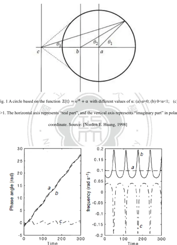
(11) frequencies and the analytical results are still not real (shown in fig.1 and fig. 2).. with different values of : (a) =0; (b) 0< <1; (c). Fig. 1 A circle based on the function. >1. The horizontal axis represents “real part”, and the vertical axis represents “imaginary part” in polar coordinate. Source: [Norden E. Huang, 1998]. Fig. 2 The left figure shows the phase angle computed by Hilbert transform, and the right figure shows the instantaneous frequency computed by the results of left figure. Source: [Norden E. Huang, 1998]. 2.

(12) Since the drawback of Hilbert transform will affect the analytical results seriously, Norden E. Huang proposed “Empirical mode decomposition (EMD)” in 1998 to solve this problem. The fundamental idea of EMD is decomposing the irregular data into several sets of nearly periodic components which called “intrinsic mode function (IMF)”, and the IMFs are symmetric to the local zero mean so that Hilbert transform can work on it. Because EMD amends the drawback of Hilbert transform successfully, a new data-analysis method “Hilbert-Huang transform (HHT)” was formally proposed in 1998. [Huang et al., 1998] Due to the fact that EMD is appropriate to analyze non-linear and non-stationary data and it also amends Hilbert transform, it has been successfully applied in many fields of researches, such as ocean waves [Hwang et al., 2003], earthquake engineering [RR Zhang et al., 2003], wind engineering [Li and Wu, 2007], biomedical engineering [Liang et al., 2005] and structured health monitoring [R Yan, 2006]. These above applications are all about nature science and engineering. However, there are more and more applications in social science in the recent years, such as financial time-series analysis [Huang et al., 2003b], transport geography [MC Chen, 2010], disease transmission [Cummings et al., 2004], and also combined with artificial neural network (ANN) to forecast crude oil price [Lean Yu et al., 2008]. In this study, we will apply HHT to analyze three sorts of time-series data: electricity consumption in NCCU, temperature in Taipei and LME gold prices.. 1.2. Purpose of research There are two major purposes why we conduct this research. The first one is analyzing the properties of electricity consumption in NCCU and temperature in Taipei by EMD, and then compared the correlation between them in different time 3.

(13) scales. Another purpose is analyzing the factors and economic meanings of the fluctuating gold prices in different time scales.. 1.3. Structure. This study is divided into 6 parts, and the brief introduction to each part is described as follows: 1.. Introduction Introducing the background and purpose of research to this study, and interpret the structure of the thesis.. 2.. Methodology Illustrating the method we used in this study, including the data-analysis method “Hilbert-Huang transform (HHT)”, statistical measures “Pearson product moment correlation coefficient”, “Kendall tau rank correlation coefficient”, ”mean period”, “variance”, “variance percentage”, “power percentage” and “LRCV”.. 3.. Data and analysis Introducing the source and format of the following data: hourly temperature, hourly electricity consumption and monthly gold prices, and analyze the decomposing components to understand the fluctuating factors of each data.. 4.. Comparison between electricity consumption and temperature Based on the measure “mean period”, we divide the components of hourly electricity consumption and hourly temperature into 4 terms, and compare the correlation between them for each term. 4.

(14) 5.. Composition of gold prices According to the results of the measure “mean period”, we divide the LME monthly gold prices into 3 terms and analyze the factors and economic meanings for each term.. 6.. Conclusion and outlook In the end, we summarize the analytical process and results, and conclude the direction of the development and application in the future.. 5.

(15) 2. Methodology. 2.1. Empirical mode decomposition. 2.1.1.. Introduction to empirical mode decomposition. Empirical mode decomposition (EMD) is a general non-linear and non-stationary data processing method which developed by [Huang et al., 1998]. Since this method is empirical, intuitive and adaptive, it is appropriate to analyze non-linear and non-stationary data. By sifting process of EMD, the irregular time series can be decomposed into an independent set of nearly periodic oscillatory modes which called “intrinsic mode functions (IMFs)”. Dissimilar to the non-linear and non-stationary data, the IMFs are based on the local characteristic time scale and vibrate in more regular modes. Due to the nearly periodic properties of the IMFs, they perhaps have some particular physical meanings; for instance, if the period of an IMF is about one day or 24 hours, it can be recognized as the daily component of the original data; likewise, an IMF with the period approximates to one week implies that the IMF is the weekly component of the original data. As these results, non-linear and non-stationary time series can be decomposed into a set of IMFs by EMD, and the IMFs are easier to analyze their own physical meanings than the original data.. 6.

(16) 2.1.2. Intrinsic mode functions and sifting process. The empirical mode decomposition (EMD) proposed by [Huang et al., 1998] is a data-analysis method which is useful to deal with non-linear and non-stationary time series. It assumes every time series can be decomposed into a set of intrinsic mode functions (IMFs). The IMFs are based on the local characteristic scale by itself, and they have to satisfy the following conditions:. (1) The IMFs have the same numbers of extrema (including maxima and minima) and zero-crossings, or differ at most by one; (2) At any point, the mean value of the upper envelope (defined by local maxima) and the lower envelope (defined by local minima) is zero; it means the IMFs are symmetric with respect to local zero mean.. We can use the sifting process to extract the IMFs from the original data by the following steps: (1) Identify all the local maxima and minima of the time series x(t) (2) Connect all the local maxima and minima by cubic spline interpolation to generate its upper envelope emax(t) and lower envelope emin(t) (3) Calculate the point-by-point averages m(t) from the upper and lower envelopes:. (4) Calculate the difference between the time series x(t) and the mean value m1(t), and get h1(t) as : h1(t) = x(t) - m1(t). 7.

(17) (5) Check the properties of h1(t): If h1(t) doesn’t satisfy the conditions of IMF, replace x(t) with h1(t) and repeat the steps from (1) to (4) until hk(t) satisfies the stopping criterion:. A typically value for SD is set between 0.2 and 0.3. On the contrary, if h1(t) satisfies the conditions of IMF, it’s set to be the first IMF and denotes h1(t) as the first component c1(t), and then we separate the IMF c1(t) from the original data x(t) to get the residue r1(t): x(t) - c1(t) = r1(t) (6) Replacing x(t) with r1(t) and repeats the steps from (1) to (5) to get c2(t).c3(t).c4(t).c5(t)………..cn(t), and finally remains the residue rn(t).. An example of sifting process is shown in fig. 3, and the IMFs and residue are shown in fig. 4. The sifting process stops by any of the following predetermined criteria: either when the component cn(t) or the residue rn(t) becomes so small that it is less than the predetermined value of substantial consequence, or when the residue rn(t) becomes a monotonic function since no more IMFs can be extracted. [Huang et al. 1998] At the end of the sifting process, the original time series can be expressed as. Where n is the number of IMFs, rn(t) is the final residue as the trend of x(t), and ci(t) represents IMFs as the independent component of x(t). The IMFs are listed from high frequency to low frequency by sifting processes, so we can regard the EMD as a filter to separate high frequency components to low frequency components. 8.

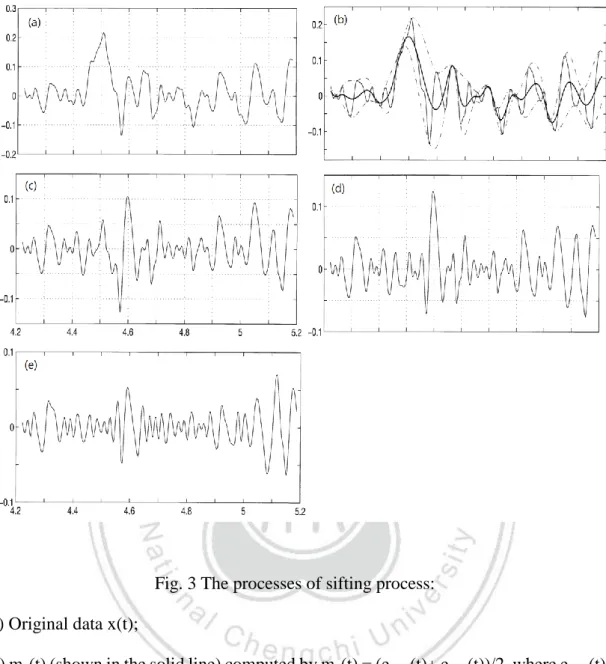
(18) Fig. 3 The processes of sifting process: (a) Original data x(t); (b) m1(t) (shown in the solid line) computed by m1(t) = (emax(t)+ emin(t))/2, where emax(t) and emin(t) are the upper and lower envelopes (both shown in the dotted line); (c) get h1(t)=x(t)-m1(t) by the 1st sifting process, but h1(t) doesn’t satisfy the properties of IMF; (d) get h2(t) by repeating sifting process again, but it is still not an IMF; (e) the 1st IMF has been extracted after repeating 9 sifting process. Source: [Norden E. Huang, 1998]. 9.

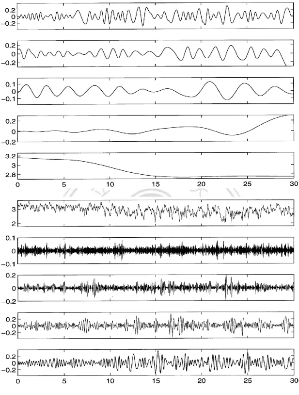
(19) Fig. 4 There are 7 IMFs (list from 2nd to 8rd lines) and one residue (list in the 9rd line) have been decomposed from the original time series (list in the 1st line) by the sifting process. Source: [Norden E. Huang, 1998]. 10.

(20) 2.1.3. Ensemble Empirical Mode Decomposition. EMD has been proved to be a useful data-analysis method by extracting IMFs from non-linear and non-stationary time series. Even though EMD is adaptive and intuitive to analyze non-linear and non-stationary time series, it still has many unsolved drawbacks. The most major and common drawbacks of EMD is the mode-mixing problem. The mode-mixing problem is defined as an IMF consists with disparate local time scales; in other words, the mode-mixing IMF includes two or more oscillatory modes which the superfluous one are similar to other IMFs. The mode-mixing problem is often caused by the intermittence signals in the original data, and a typical example to illustrate it is shown in fig. 5 and fig. 6. On account of the mode-mixing problem in EMD, sometimes the IMF can not represent its own meanings clearly; thus, EEMD has been proposed by [Wu and Huang, 2004] for solving the mode-mixing problem by adding white noise. We know that each observed data are mixed with true time series and noise; since the noise contains wider frequency domain, the ensemble mean of the observed data is close to the true time series. For instant, the white noise contains whole nature frequency and its ensemble mean of the residue is close to zero (shown in fig. 7 and fig. 8). Accordingly, it is reasonable to add white noise to the original data and we can still extract the true signal by computing the ensemble mean; as these reasons, the additional white noise does not obviously affect the ensemble mean between the upper and lower envelopes in the sifting process. The procedure of EEMD is shown as the follows: (1) Adding a time-series white noise to the original data (2) Decomposing IMF from the data with additional white noise 11.

(21) (3) Repeat the above two steps iteratively, and add different white noise for each time. Finally we obtain the ensemble means of corresponding IMFs of the decompositions.. However, there is a well-established statistical rule proved by [Wu and Huang, 2004] to control the parameters of the additional white noise:. Where N is the ensemble number, ε is the amplitude of the additional white noise, and εn is the final standard deviation of error. The standard deviation of error is defined as the difference between the input signal and the corresponding IMFs. The results compared between EMD and EEMD are shown in fig.5, fig.6 and fig.9. In this study, the ensemble number N is set to be 100 and the ε is set to be 0.1. As these results, the procedure of additional white noise can successfully fill the original data with uniform frequency domain and eliminate most of the mode-mixing problems in IMFs. Therefore, EEMD is a substantial improvement over the original EMD.. 12.

(22) Fig. 5 The original data is based on sine wave and contains the intermittence signals with higher frequency and the first sifting process. Source: [Wu and Huang, 2004]. Fig. 6 The IMFs and the residue extracted from the data (see fig. 5), and C1 obviously includes two oscillatory modes which called mode-mixing problem. Source: [Wu and Huang, 2004] 13.

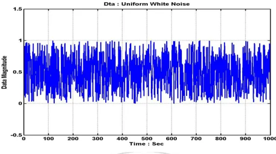
(23) Fig. 7 The original data of uniform white noise recorded in 1000 seconds. [Source: Data Analysis Center, NCU]. Fig. 8 The IMFs and the residue decomposed from the uniform white noise with SD=1, and the mean value of residue is about zero. [Source: Data Analysis Center, NCU] 14.

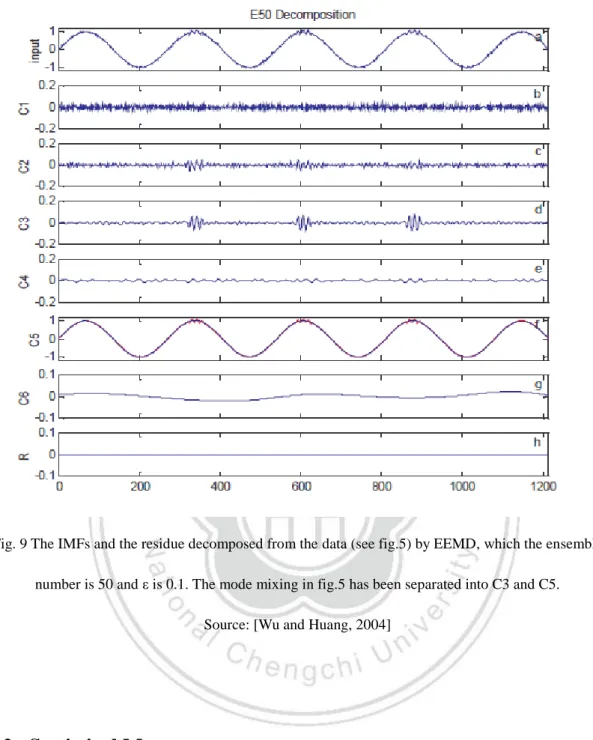
(24) Fig. 9 The IMFs and the residue decomposed from the data (see fig.5) by EEMD, which the ensemble number is 50 and ε is 0.1. The mode mixing in fig.5 has been separated into C3 and C5. Source: [Wu and Huang, 2004]. 2.2. Statistical Measures. We use the following statistical measures to analyze the IMFs and residues: mean period, Pearson product moment correlation coefficient, Kendall tau rank correlation coefficient, variance, variance percentage, power percentage and LRCV. The definitions of these statistical measures are illustrated as follows.. 15.

(25) 2.2.1.. Mean period. The mean period is defined by “inverse of mean frequency”, and the mean frequency is the average of the “instantaneous frequency”. The instantaneous frequency is computed by Hilbert-Huang transformation (HHT), and the processes for computing instantaneous frequency by HHT are shown as the follows: We can extract the IMFs from the original data by EMD or EEMD. Since the IMFs are symmetric to the local zero mean, it’s available to use Hilbert transformation to compute the time-series imaginary part Y(t):. Where X(τ ) is the value of the original time-series data at t=τ , Y(t) is the corresponding imaginary part, and p.v. indicates the Cauchy principal value of singular integral. As the X(t) and Y(t) are the corresponding real part and imaginary part, they are allowed to form the time-series complex conjugate pairs in the polar coordinate:. Where a(t) is the time-series amplitudes in the polar coordinate, its definition is:. And (t) is the time-series phase in the polar coordinate, its definition is:. Since X(t) and Y(t) are both instantaneous values, (t) can indicate the changing value of the phase between two continue points. The instantaneous frequency can be computed by (t) on the time interval differential as follows:. As the instantaneous frequency is defined by differential, it is useful to compute 16.

(26) the frequencies or periods of the non-linear and non-stationary time series. We can compute the mean period of the IMFs by instantaneous frequency, and analyze the meanings or properties of them. In addition to analyzing the properties of the IMFs, the mean period is also an important measure to divide the IMFs into several groups. On the other hand, it is meaningless to compute the mean period of the residue because it is a monotonic function. Due to this reason, we only compute the mean period of the IMFs in this study.. 2.2.2. Pearson product moment correlation coefficient. Pearson product moment correlation coefficient is a statistical measure which is often used to compare the degree of linear dependence between two variables. The definition of Pearson product moment correlation coefficient between two variables X and Y (. ) is shown as the follows:. The σ is the standard deviation which defined as. Where X is the value at any point of the variable,. is the average of the. variable X, and E indicates the expectation. The cov(X, Y) is the covariance of the variables X and Y which divided by the product of their standard deviations obtained as:. The Pearson correlation coefficient always ranges from −1 to 1. The larger the value of Pearson correlation is, the higher the linear correlation between two variables is. The different sorts of relationship between two variables and their corresponding 17.

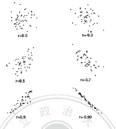
(27) values of the correlation coefficient are shown in fig. 10. A value of 1 shows that all the data of X and Y are either keeping increasing or decreasing in the same interval, and there must be a linear equation that describes the relationship between X and Y perfectly. A value of −1 shows that all the data of X and Y are varying in the opposite direction, and the relationship between X and Y is strongly positive correlation. A value of zero means there is no linear correlation between X and Y. The extent of the correlation in different ranges of Pearson product moment correlation is shown in table.1.. Table. 1 The extent of linear correlation represented by different ranges of Pearson product moment correlation coefficient. Source: [Linear statistical models, Philip B. Ender, UCLA]. Correlation. Negative. Positive. None. −0.09 to 0.0. 0.0 to 0.09. Small. −0.3 to −0.1. 0.1 to 0.3. Medium. −0.5 to −0.3. 0.3 to 0.5. Large. −1.0 to −0.5. 0.5 to 1.0. 18.

(28) Fig. 10 Different sets of the points and their corresponding values of Pearson product moment correlation coefficients (r). Source: [Linear statistical models, Philip B. Ender, UCLA]. 2.2.3.. Kendall tau rank correlation coefficient. In statistics, Kendall tau rank correlation coefficient is used to measure the association between two variables. Different from Pearson product moment correlation coefficient, Kendall tau rank correlation coefficient is a measure of rank correlation; hence, it is used to compare the ordering of the concordant rank between two variables. The Kendall tau rank correlation coefficient is defined as:. 19.

(29) Where n is the number of the data points. The concordant and discordant pairs are defined as follows: for two variables X and Y, if the corresponding values between them are in a concordant ranking, such as both Xi > Xj and Yi > Yj, or both Xi < Xj and Yi < Yj, the two variables are said to be concordant pairs. On the contrary, if the corresponding value between them are in a discordant rank, such as Xi > Xj but Yi < Yj, or Xi < Xj but Yi > Yj, the two variables are said to be discordant pairs. Kendall tau rank correlation coefficient must range from -1 to +1, and the values of +1, -1 and zero implies different ordering of ranking. A value of +1 means the ranking between two variables is perfectly agreement, and the number of discordant pairs is zero. A value of -1 means the ranking between two variables is perfectly disagreement, and the number of concordant pairs equals to zero. If the value approximates to zero, it means the two variables are independent to each other.. 2.2.4.. Variance. Since the variance percentage and power percentage are both defined by variance, we introduce three statistical measures together in this part. We first introduce variance. Followed by variance percentage and finally power percentage. The definition of variance is the square mean of the difference between the data and ensemble average, which is shown as follows:. Where X is the value of the data, μ is the ensemble average, and E indicates the except value. In probability theory and statistics, variance is used to determine the degree of dispersing for a set of points. The degree of dispersing means how far the data locate 20.

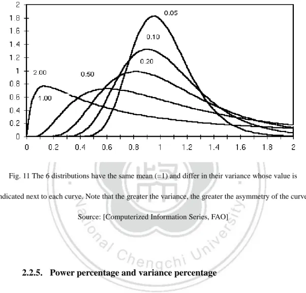
(30) from the ensemble average, so variance is a useful measure to show the data aggregate or disperse from the ensemble average. Typical examples that explain difference distributing data and their corresponding variance are shown in fig.11.. Fig. 11 The 6 distributions have the same mean (=1) and differ in their variance whose value is indicated next to each curve. Note that the greater the variance, the greater the asymmetry of the curve. Source: [Computerized Information Series, FAO]. 2.2.5. Power percentage and variance percentage. The definitions of power percentage and variance percentage are shown as follows:. 21.

(31) Owing to the definitions, power percentage and variance percentage can show the degree of weighting for each IMF or residue with different perspectives; power percentage is based on the original data and variance percentage is based on the summation of each component. Nevertheless, the summed up variance of all IMFs and residue is not totally equivalent to the variance of the original data due to the round-off errors, additional white noise, and cubic spline end conditions in EEMD [Peel et al., 2005]. Since variance is used to determine how far the data points locate from the local mean, both power percentage and variance percentage can show the degree of weighting as the percentage measures for each component. The larger the two percentage measures are, the more important the component is. Thus, these two measures are useful to determine which component is worth analyzing.. 2.2.6. LRCV. The measure “LRCV” is the abbreviation of “logarithm of the ratio of consecutive financial variable values” [Huang et al., 2003b]. LRCV is often used to analyze financial time-series data, its definition is shown as follows:. Where Sn is the value of the original data at the nth time step, and logarithm is the natural logarithm. The value of LRCV represents variability between two continue time steps, and higher values of LRCV correspond to sharper fluctuations in the original data. This measure is only used to compare the volatility of the original monthly gold prices with the high frequency term in section 6. 22.

(32) 3. Data and analysis. The hourly electricity consumption, hourly temperature and LME monthly gold prices can be decomposed into a set of IMFs with different time scales and the residues by EEMD. Since there are lots of components decomposed from the data, we must to sort out the significant components which are more meaningful to analyze. The statistical measures “power percentage” and “variance percentage” are used to determine the significant components, and the correlation coefficients “Pearson product moment correlation coefficient” and “Kendall tau rank correlation coefficient” are used to compare the correlation between the significant components with the original data. Among all the significant components, the IMFs can be indicated their own specific meanings by the statistical measure “mean period”, and the residues exhibit deterministic long-run properties as the trends of the original data [Huang et al., 1998]. As these reasons, we can find the characteristics of the original data by analyzing the IMFs and the residues. In this section, we introduce the data source for a start, and then analyze the meanings of the significant components for each data part by part, and finally summarized the results of the analysis.. 23.

(33) 3.1. Data. 3.1.1. Hourly electricity consumption in NCCU. The hourly electricity consumption is supplied by [Office of General Affairs, NCCU]. The recording period of the data starts from January 28th, 2008 to February 3rd, 2010. According to the different sampling frequency, the data are divided into two types: hourly electricity consumption and daily electricity consumption. Both the two types of data record the electricity consumption from five major electricity meters in NCCU, which named GCB2, GCB3, GCB5, GCB6, and GCB10. The five electricity meters record the electricity consumption for different buildings as follows: GCB2-Information Building, GCB3-Research Building, GCB5-College of Commerce Building, GCB6-CiSian Building, GCB10-General Building of Colleges. Since the electricity consumption of Information Building, College of Commerce Building and General Building of Colleges are higher than others, and the hourly data reveals more information and details than the daily data, we choose the hourly data of GCB2, GCB5 and GCB10 to analyze the electricity consumption in NCCU. The duration of the analytical data we select starts from March 1st, 2008 to June 30th, 2008 because the electricity consumption of 2nd semester is always much higher than 1st semester in NCCU.. 3.1.2. Hourly temperature in Taipei. The data “hourly temperature in Taipei” is picked from the hourly atmospheric data recorded by the weather station “Taipei (6920)”, which the original data are 24.

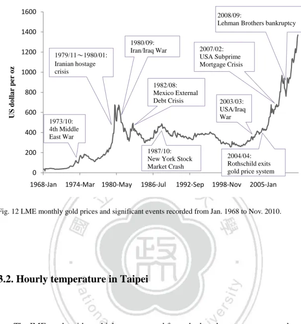
(34) downloaded from [Data Bank for Atmospheric Research (DBAR), NTU]. The analytical period of the hourly temperature we select is as same as the hourly electricity consumption. The hourly atmospheric data contain 152 rows, and each row corresponds to diverse atmospheric measures. According to the illustration of hourly atmospheric data provided by DBAR, the measure from 29th row to 33th row called “dry bulb temperature”, which shows the average hourly temperature in Taipei, and it is the analytical data we need in this study. Due to the same sampling frequency and recording period for the two sorts of data, it is available to compare the correlation between the electricity consumption and temperature in NCCU during the same interval of time.. 3.1.3. Monthly gold price. The gold price data are downloaded from the website named [KITCO (www.kitco.com)], and the original data is recorded by London Metal Exchange (LME) with the unit of US dollar per oz ($/ounce). The original monthly gold prices and the corresponding significant events are shown in fig. 11. There are many types of gold price data recorded by LME, such as hourly data, monthly data, and yearly data. In this study, we choose the monthly gold prices to analyze for the following reasons. Owing to the monthly data equivalent to approximately 24 years, it can perform more information and factors in the long run as it shows longer time variance than hourly data and extracts more details than yearly data (1833 to 1999). Thus, monthly data can best present the details in long run (fig. 12). 25.

(35) 1600. 2008/09: Lehman Brothers bankruptcy. 1400. US dollar per oz. 1200 1000. 1979/11～1980/01: Iranian hostage crisis. 1980/09: Iran/Iraq War. 2007/02: USA Subprime Mortgage Crisis. 1982/08: Mexico External Debt Crisis. 800 600 400. 1973/10: 4th Middle East War 1987/10: New York Stock Market Crash. 200 0 1968-Jan. 1974-Mar 1980-May. 1986-Jul. 1992-Sep. 2003/03: USA/Iraq War. 2004/04: Rothschild exits gold price system. 1998-Nov. 2005-Jan. Fig. 12 LME monthly gold prices and significant events recorded from Jan. 1968 to Nov. 2010.. 3.2. Hourly temperature in Taipei. The IMFs and residue which are extracted from the hourly temperature are shown in fig.13 and fig.14. Also, the statistical measures are shown in table. 2. Among all the components of the hourly temperature, the most significant one is the residue because its weighting percentage and correlation coefficients are both the largest. The power percentage of residue is about 46% and variance percentage is about 60%. The Pearson and Kendall correlation coefficient for each is about 0.702 and 0.513. In addition to the residue, another significant component is IMF4, which is with the mean period around 24 hours. The power percentage and variance percentage of IMF4 are 13.5% and 17.38%, and both of them are the largest above all the IMFs. On the other hand, the Pearson and Kendall correlation coefficient of IMF4 for each is 0.432 26.

(36) and 0.255; the Pearson correlation coefficient is the highest, but the Kendall correlation coefficient is lower than IMF7 and IMF8. Since the residue and the IMF4 are more essential than other components for hourly temperature, their meanings and properties are claimable to analyze. The residue exhibits the trend of the original data in the whole duration. The value of residue is around 16℃ at the beginning, and finally it reaches 30℃; the total difference of the residue nears 14℃, and it is close to the difference of the original data which approaches to 15℃. The changing value of the original data is almost as same as the residue, so the residue can only represent the difference of the original data without any fluctuation in the long run. The IMF4 is the most significant component above all the IMF. The mean period of IMF4 almost takes 24 hours, and the amplitudes vibrate between -5℃ to 5℃. As the mean period of IMF4 equals to 24 hours, we can treat it as the daily component of the hourly temperature. The hourly temperature is often higher in afternoon and lower in midnight. Hence, the values change in the circles with the mean period is 24 hours. Consequently, the amplitudes of IMF4 show the diurnal temperature with the range less than 5℃ during March to June. By analyzing the components and the statistical measures, we can conclude that the residue and IMF4 are the significant components of the hourly temperature. The residue shows the trend of the hourly temperature in the long run, and IMF4 shows the ranges of diurnal temperature in this period. Above these reasons, the residue and IMF4 can reveal different meanings in different time scales, and both of the meanings are significant to the hourly temperature.. 27.

(37) data. 40. imf3. imf2. imf1. 10 1 -1 1 -1 2 -2. imf4. 5. -5. imf5. 2. -2 3/01. 4/01. 5/01. 6/01. 6/30. Date. imf11. imf10. imf9. imf8. imf7. imf6. Fig. 13 The original data and IMF1 to IMF5 extracted from the hourly temperature.. 2 -2 2 -2 2 -2 1 -1 1 -1. 0.5 -0.5. res.. 30 20 3/01. 4/10. 5/01. 6/01. 6/30. Date. Fig. 14 The IMF6 to IMF11 and the residue extracted from the hourly temperature. 28.

(38) Table. 2 The statistical measures of the components decomposed from hourly temperature. Mean. Mean. Pearson. Kendall. Power. Variance. Variance period (hr). period (day). coefficient. coefficient. percentage percentage 20.5. Data IMF1. 3.82. 0.159. 0.070. 0.038. 0.051. 0.25%. 0.32%. IMF2. 7.17. 0.299. 0.126. 0.078. 0.071. 0.35%. 0.45%. IMF3. 12.62. 0.526. 0.289. 0.141. 0.458. 2.24%. 2.88%. IMF4. 24.60. 1.025. 0.432. 0.255. 2.768. 13.50%. 17.38%. IMF5. 50.58. 2.107. 0.255. 0.156. 0.242. 1.18%. 1.52%. IMF6. 83.97. 3.499. 0.315. 0.204. 0.732. 3.57%. 4.59%. IMF7. 132.85. 5.536. 0.371. 0.260. 0.608. 2.96%. 3.81%. IMF8. 226.86. 9.453. 0.363. 0.242. 0.726. 3.54%. 4.56%. IMF9. 370.72. 15.447. 0.329. 0.204. 0.407. 1.99%. 2.56%. IMF10. 591.40. 24.642. 0.272. 0.166. 0.269. 1.31%. 1.69%. IMF11. 750.10. 31.254. 0.156. 0.095. 0.139. 0.68%. 0.87%. 0.702. 0.513. 9.460. 46.14%. 59.38%. 15.93. 77.71%. 100.00%. Residue Sum. 29.

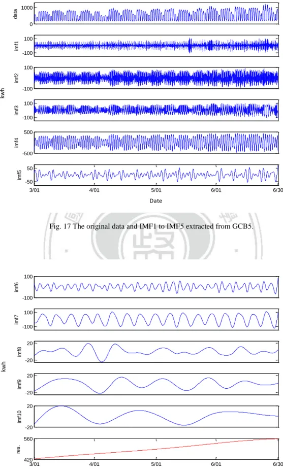
(39) 3.3. Hourly electricity consumption in NCCU. The hourly electricity consumption in NCCU includes three sets of data: GCB2, GCB5 and GCB10. The three electricity meters record the hourly data in the different buildings, so the fluctuating properties of them are a bit of different; such as the basic electricity consumption, and the diurnal difference of electricity consumption. Besides these different properties, the significant components are the same for the three sets of data; they are the daily components (IMF4) and the weekly components (IMF7). The residues are also significant to the hourly electricity consumption, but their weighting percentages are distinct for them. The original data, IMFs, residues and the statistical measures are shown in fig.15, fig.16 and table.3 for GCB2; fig.17, fig.18 and table.4 for GCB5; fig.19, fig.20 and table.5 for GCB10. Since the factors of the hourly electricity consumption are too complicated to analyze, we separate the analytical process in three parts: Firstly, describe the properties of the original data. Secondly, analyze the significant IMFs, and finally analyzing the residue for each electricity meter. After interpreting the meanings for each. part,. we. will. summarize. the. 30. results. and. make. the. conclusion..

(40) data. 1000. 200. imf1. 50 -50. imf2. kwh. 50 -50. imf3. 100. -100. imf4. 200 -200 3/01. 4/01. 5/01. 6/01. 6/30. Date. imf5. Fig. 15 The original data and IMF1 to IMF4 extracted from GCB2.. 50 -50. imf6. 50. -50. kwh. imf7. 100. imf8. -100 10 -10. imf9. 20 -20. res.. 460. 320 3/01. 4/01. 5/01. 6/01. Date. Fig. 16 The IMF5 to IMF9 and the residue extracted from GCB2.. 31. 6/30.

(41) Table. 3 The statistical measures of the components decomposed from GCB2. Mean. Mean. Pearson. Kendall. Power. Variance. Variance period (hr). period (day) coefficient coefficient. percentage percentage 21123.7. Data IMF1. 3.99. 0.166. 0.094. 0.011. 158.9. 0.75%. 0.95%. IMF2. 6.32. 0.264. 0.168. 0.073. 320.0. 1.52%. 1.91%. IMF3. 12.85. 0.535. 0.628. 0.422. 817.7. 3.87%. 4.87%. IMF4. 24.00. 1.000. 0.840. 0.643. 11259.9. 53.30%. 67.06%. IMF5. 53.31. 2.221. 0.233. 0.097. 390.0. 1.85%. 2.32%. IMF6. 84.00. 3.500. 0.249. 0.133. 443.7. 2.10%. 2.64%. IMF7. 163.96. 6.832. 0.309. 0.183. 1595.0. 7.55%. 9.50%. IMF8. 375.68. 15.653. 0.089. 0.043. 26.8. 0.13%. 0.16%. IMF9. 758.15. 31.590. 0.090. 0.051. 105.2. 0.50%. 0.63%. 0.257. 0.167. 1672.3. 7.92%. 9.96%. 16789.6. 79.48%. 100.00%. Residue Sum. 32.

(42) data. 1000. imf1. 0 100 -100. imf2. 100. imf3. kwh. -100 100 -100. imf4. 500. imf5. -500 50 -50 3/01. 4/01. 5/01. 6/01. 6/30. Date. Fig. 17 The original data and IMF1 to IMF5 extracted from GCB5.. imf6. 100. imf7. -100 100 -100. imf8. 20. kwh. -20. imf9. 20 -20. imf10. 20. -20. res.. 560. 420 3/01. 4/01. 5/01. 6/01. Date. Fig. 18 The IMF6 to IMF10 and the residue extracted from GCB5. 33. 6/30.

(43) Table. 4 The statistical measures of the components decomposed from GCB5. Mean. Mean. Pearson. Kendall. Power. Variance. Variance period (hr). period (day) coefficient coefficient. percentage percentage 76993.72. Data IMF1. 4.36. 0.182. 0.090. -0.040. 659.73. 0.86%. 1.04%. IMF2. 6.14. 0.256. 0.151. 0.057. 1327.92. 1.72%. 2.09%. IMF3. 10.46. 0.436. 0.623. 0.434. 1836.9. 2.39%. 2.89%. IMF4. 24.00. 1.000. 0.909. 0.702. 52970.32. 68.80%. 83.29%. IMF5. 48.88. 2.037. 0.181. 0.087. 413.74. 0.54%. 0.65%. IMF6. 83.85. 3.494. 0.211. 0.127. 616.31. 0.80%. 0.97%. IMF7. 164.13. 6.839. 0.279. 0.190. 3915.51. 5.09%. 6.16%. IMF8. 371.71. 15.488. 0.096. 0.068. 60.96. 0.08%. 0.10%. IMF9. 596.87. 24.870. 0.081. 0.052. 91.13. 0.12%. 0.14%. IMF10. 1010.34. 42.098. 0.059. 0.035. 94.19. 0.12%. 0.15%. 0.139. 0.118. 1608.91. 2.09%. 2.53%. 63595.63. 82.60%. 100.00%. Residue Sum. 34.

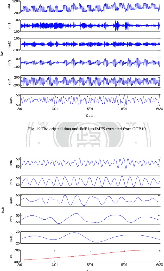
(44) data. 1200. 200. imf1. 100. -100. imf2. 100. imf4. imf3. kwh. -100 100 -100 200 -200. imf5. 50 -50 3/01. 4/01. 5/01. 6/01. 6/30. Date. imf7. imf6. Fig. 19 The original data and IMF1 to IMF5 extracted from GCB10.. 50 -50 50 -50. imf8. 50. imf9. kwh. -50 50 -50. imf10. 20. -20. res.. 700. 400 3/01. 4/01. 5/01. 6/01. Date. Fig. 20 The IMF6 to IMF10 and the residue extracted from GCB10. 35. 6/30.

(45) Table. 5 The statistical measures of the components decomposed from GCB10. Mean. Mean. Pearson. Kendall. Power. Variance. Variance period (hr). period (day) coefficient coefficient. percentage percentage 40292.93. Data IMF1. 3.87. 0.161. 0.128. 0.056. 482.68. 1.20%. 1.61%. IMF2. 5.80. 0.242. 0.140. 0.083. 308.41. 0.77%. 1.03%. IMF3. 17.98. 0.749. 0.664. 0.500. 1369.12. 3.40%. 4.55%. IMF4. 24.01. 1.000. 0.762. 0.555. 15431.21. 38.30%. 51.33%. IMF5. 57.54. 2.398. 0.164. 0.094. 402.53. 1.00%. 1.34%. IMF6. 88.98. 3.707. 0.273. 0.170. 707.28. 1.76%. 2.35%. IMF7. 173.46. 7.227. 0.323. 0.209. 1964.82. 4.88%. 6.54%. IMF8. 294.86. 12.286. 0.232. 0.148. 598.98. 1.49%. 1.99%. IMF9. 733.18. 30.549. 0.226. 0.145. 1535.6. 3.81%. 5.11%. IMF10. 978.93. 40.789. 0.185. 0.123. 65.96. 0.16%. 0.22%. 0.417. 0.279. 7198.93. 17.87%. 23.94%. 30065.51. 74.62%. 100.00%. Residue Sum. 3.3.1. Original data. The original data are not totally the same for the three sets of data since the number of floors and the structure of electricity consumption are different in these buildings. The basic electricity consumption has concerned with the number of floors, and the diurnal difference between peak hours and off-peak hours are related to the 36.

(46) structure of electricity consumption. We discuss the basic electricity consumption at first. Basically, electricity consumption means the data which is recorded during off-peak hours, such as midnight and early morning; since there are no classes or activities in these durations, the electricity consumption is the minimum value to maintain the basic operation of the buildings. The basic electricity consumption and the number of floors are shown in table.6. Above all, the values of the basic electricity consumption, the largest one is GCB10 owing to the most number of floors in General Building of Colleges. Nevertheless, the basic electricity consumption of GCB2 and GCB5 are both approximate to 200 kwh, but the number of floors are totally different between them. Perhaps it is caused by the computer rooms in Information Building. Because the computer rooms need to keep consuming large power to maintain their operation, the basic electricity consumption of GCB2 is much larger than other buildings which their number of floors is similar to Information Building. Except for the basic values, the diurnal difference of electricity consumption between peak hours and off-peak hours are not totally the same for these buildings, either. The peak hours starts from 10:00 to 16:00, and the classes usually arrange during this period in weekdays. Other periods are the off-peak hours (including weekends). The difference between peak hours and off-peak hours ranges from 400 kwh to 800 kwh for GCB2, ranges from 500 kwh to 1000 kwh for GCB5, and ranges from 300 kwh to 600 kwh for GCB10. The values of GCB2 and GCB10 are less than GCB5, these results imply that the electricity consumption for teaching or other activities are less in Information Buildings and General Building of Colleges, but much more in College of Commerce Building.. 37.

(47) Table. 6 Basic electricity consumption, number of floors and difference of diurnal electricity consumption shown by each building. Difference of Basic electricity Buildings (electricity meter). Number of floors. diurnal electricity consumption consumption. Information building 7. 200 kwh. 400~800 kwh. 13. 200 kwh. 500~1000 kwh. 18. 200~400 kwh. 300~600 kwh. (GCB2) Colleges of commerce building (GCB5) General buildings of Colleges (GCB10). As these results we analyze from the original data, the electricity consumption for the buildings can be described as following: the electricity consumption for teaching is the highest in College of Commerce Building, and the basic electricity consumption is the highest in General Building of College. However, the basic electricity consumption of Information building nearly equals to College of Commerce Building, but the electricity consumption for teaching is less than it.. 3.3.2. Significant IMFs and statistics. For the hourly electricity consumption, the most significant components are the daily components with the mean periods around 24 hours. Another is the weekly components with the mean periods approach to one week. 38.

(48) The daily components are noted as IMF4 in the three sets of data (GCB2, GCB5 and GCB10), and all of them have the highest correlation and the largest weighing percentage. In addition, their mean period is close to 24 hours in IMF4. For the three sets of data, Pearson correlation coefficients of the daily components ranges from 0.7 to 0.9, and Kendall correlation coefficients ranges from 0.5 to 0.7. The power percentage of the daily components ranges from 38% to 68%, and variance percentage ranges from 50% to 83%. Because the mean period of the daily components is close to 24 hours, they can reveal the difference of the electricity consumption during one day. For example, the amplitudes of IMF4 is about 500 kwh for GCB5, and it approaches to 200 kwh for GCB2 and GCB10; this means the diurnal difference of electricity consumption is about 500 kwh for College of Commerce Building, and is close to 200 kwh for General Building of Colleges and Information Building. These results are similar to the difference between peak hours and off-peak hours from the original data (see 3.3.1.). Except for the daily components, weekly components are also the significant IMFs since the power percentage and variance percentage are only lower than the daily components. The weekly components with mean periods approximate to one week, and all of them are IMF7 for the three electricity meters. The power percentage of the weekly components ranges from 4% to 9%, and the variance percentage ranges from 6% to 10%; the Pearson correlation coefficients is about 0.3, and Kendall correlation coefficients is about 0.2 for the three electricity meters. Since most of the classes distribute during weekdays, there is a large difference of electricity consumption between weekdays and weekends. Hence, the weekly components can represent the difference of electricity consumption between weekdays and weekends by the amplitudes. The amplitudes of IMF7 is about 50 kwh for GCB10, and about 100 kwh for GCB2 and GCB5; it implies that the demand of electricity consumption in weekdays is much more 39.

(49) in College of Commerce and Information Building, but less demand in General. Building of Colleges. On the other hand, the amplitudes of higher frequency components (IMF1, IMF2 and IMF3) are distributed as the normal distribution. Since the normal distribution is often concluded as random walk, the fluctuating properties of higher frequency components are similar to random walk in the macroscopic perspective, and their mean amplitudes are about zero (fig.21). The power percentage and variance percentage of IMF1, IMF2 and IMF3 only contribute 7% totally at most, so they are not as important as the daily components and weekly components.. GCB2: IMF1. GCB2: IMF3. 1. 1. 0.5. 0.5. 0.5. 0 -70 Normalized number. GCB2: IMF2. 1. 0. -70. 0 -80. GCB5: IMF1. 0. 80. 0 -170. GCB5: IMF2 1. 1. 0.5. 0.5. 0.5. 0. 120. 0 -100. GCB10: IMF1. 0. 100. 0 -230. GCB10: IMF2 1. 1. 0.5. 0.5. 0.5. 0. 100. 0 -70 0 70 Distribution of amplitudes. 0. 230. GCB10: IMF3. 1. 0 -100. 170. GCB5: IMF3. 1. 0 -120. 0. 0 -350. 0. 350. Fig. 21 The normalized histogram is shown in blue bar, and the corresponding normal distribution is shown in red line.. 40.

(50) According to the results, the daily and weekly components are provided with both importance and essential meanings for the hourly electricity consumption. In the next section, the compositions of electricity consumption are based on daily and weekly components.. 3.3.3. Residues. For the three electricity meters, all the residues represent the increasing trend as what the residue of hourly temperature does. But their weighting percentages are dissimilar for each others. The power percentage and variance percentage of the residues for each is 7.92% and 9.96% for GCB2, 2.09% and 2.53% for GCB5, 17.87% and 23.94% for GCB10. Based on the power percentage and variance percentage, the residue of GCB10 is more significant than GCB5 and GCB2. This result shows the basic electricity consumption is steadier and lacks of smooth change in College of Commerce Building and Information Building during March to June. Quite the other way, the residue of GCB10 almost raises 300 kwh in the whole duration, so its basic electricity consumption also keeps increasing evidently. We can conclude that residue reveals the basic electricity consumption by comparing it with the original data. According to we analyze from the residues, the basic electricity consumption is the largest increase in General Building of Colleges, and raises less in College of Commerce Building and Information Building. These results are similar to what we analyzed from the original data.. 41.

(51) 3.4. Monthly gold price. There are eight IMFs and one residue exacted from the monthly gold price data by EEMD. The original data and the results of decomposition are shown in fig.22, and the statistical measures are listed in table.7. All the IMFs can be extracted and listed from high frequency to low frequency by the sifting processes. Except for the residue, the IMF with the highest frequency is IMF1 which is extracted at first and the IMF with the lowest frequency is IMF8 which is extracted at last.. res.. IMF8. IMF7. IMF6. IMF5. IMF4. IMF3. IMF2. IMF1. data. 1400 0 50 -50 50 -50 50 -50 100. -100 100 -100 100 -100 100 -100 200 -200 900 0 1968M1. 1976M5. 1984M9. 1992M1. 2000M5. Date Fig. 22 The IMFs and residue exacted from LME monthly gold prices. 42. 2008M9.

(52) The frequencies and amplitudes of the IMFs vary with time since the original data is non-linear and non-stationary. For the IMFs of the monthly gold prices, the lower the frequency is, the larger the amplitude of the IMFs is. For example, the amplitudes of IMF1 to IMF3 range from nearly around $50/ounce to -$50/ounce and they are the highest in frequency but the lowest in amplitude among all the IMFs. On the contrary, the IMF8 carries the lowest frequency and the largest amplitude range from $200/ounce to -$200/ounce which is only smaller than the residue. The amplitude of the residue keeps increasing from $187/ounce at Jan. 1968 and finally it reaches $837/ounce at Nov. 2010.. Table. 7 The statistical measures of the components decomposed from LME monthly gold prices. Mean period. Pearson. Kendall. (month). correlation. correlation. Power. Variance. percentage. percentage. Variance. 56,815.28. Data IMF1. 3.07. 0.067. 0.021. 121.75. 0.21%. 0.18%. IMF2. 5.99. -0.070. 0.009. 105.38. 0.19%. 0.16%. IMF3. 9.90. -0.065. -0.001. 131.49. 0.23%. 0.19%. IMF4. 17.17. 0.231. 0.150. 292.81. 0.52%. 0.43%. IMF5. 46.82. 0.303. 0.243. 505.44. 0.89%. 0.75%. IMF6. 73.57. 0.328. 0.228. 948.88. 1.67%. 1.40%. IMF7. 257.50. 0.301. 0.112. 1,715.31. 3.02%. 2.53%. IMF8. 484.97. 0.414. 0.308. 20,796.14. 36.60%. 30.67%. 0.701. 0.419. 43,189.62. 76.02%. 63.70%. 67,806.82. 119.35%. 100.00%. Residue Sum. 43.

(53) For the results of decomposition, the most dominant component is the residue, and the second one is IMF8. The Kendall and Pearson correlation coefficients of the residue are 0.419 and 0.701, indicating the highest correlation between original data in all the components; simultaneously, its variance percentage approximates 63.7% which is also the most essential one. Besides the residue, the second important component is IMF8. The mean period of IMF8 is approach to 485 months, which is nearly as long as the original data. The Kendall and Pearson coefficients of IMF8 are 0.308 and 0.414. On account of the slowly vibrating behavior of IMF8, both the values of two correlation coefficients are smaller than that of residue. As the reasons we mention above, IMF8 and the residue are the two major components for the monthly gold prices since they contribute totally 94.37% of variance percentage. Especially the residue, since it keeps increasing as the original data does, its Kendall correlation coefficient is the highest above all. On the other hand, there are only 0.52% of variance percentage contributed by IMF1 to IMF3 which carry higher frequency than other IMFs. We can come up with the result that the higher the frequency of IMF is, the lower the importance it is; due to this result, the IMFs will be divided into groups as the different mean periods in the next section.. 3.5. Conclusion of analysis. According to these results, we can summarize the conclusion as follows. For hourly electricity consumption, the similar properties of the three electricity meters are the significant components and the residues, and the dissimilar properties of them are the basic electricity consumption and diurnal difference between peak hours and off-peak hours. The significant components of the hourly electricity consumption are 44.

(54) the daily components and the weekly components, and the residues of them both keep increasing as the trend of the hourly temperature does. For monthly gold prices, the significant components are residue and IMF8, where the residue is a monotonic function and the mean period of IMF8 is the longest above all. The significant components are both important and meaningful to the original data, so they can reveal the major factors of the original data. Since these significant components vibrate in different time scale, we will select some IMFs as the reasonable boundaries to divide them into groups and analyze the further results.. 45.

(55) 4. Comparison between electricity consumption and temperature. The decomposed components and analyzed results of the hourly electricity consumption and the hourly temperature have been shown in Section 3. In this section, the IMFs are divided into high frequency term, mid frequency term and low frequency term based on the mean period. The IMFs and the residues are separated into four terms for each data, and they are shown in fig.23, fig.24, fig.25 and fig.26; the statistical results are shown in table.8, table.9, table.10 and table.11. The unit of x-axis is date, and unit of y-axis is kwh for electricity consumption and Celsius for temperature. The IMFs classified to the low frequency term are sorted out as the mean period exceeded 7 days; the IMFs classified to the mid frequency term are chosen as the mean period over 24 hours but within or less than 7 days; the IMFs classified to the high frequency term are chosen as the mean period within or less than 24 hours. Since the natural factor, like temperature, and man-made factors, such as the use of class room during classes or activities, are the major influences affecting on the hourly electricity consumption, we can analyze the correlation between the electricity consumption and temperature in different time scales by dividing the IMFs and residues into four terms, and describe the driven factors for each one.. 46.

(56) data. 1000. 200. high. 400. -400. mid. kwh. 200. -200. low. 40. -40. trend. 500. 300 3/01. 4/01. 5/01. 6/01. 6/30. Date. Fig. 23 The four terms divided from the components of GCB2.. Table. 8 The statistical measures of the terms divided from GCB2. Mean period Pearson. Kendall. GCB2. Power. Variance. Variance (day). coefficient Coefficient. percentage percentage 21123.697. Data High frequency term. 1.001. 0.872. 0.662. 16274.759. 77.05%. 76.52%. Mid frequency term. 6.469. 0.395. 0.232. 3158.700. 14.95%. 14.85%. Low frequency term. 20.939. 0.109. 0.044. 161.662. 0.77%. 0.76%. 0.257. 0.167. 1672.289. 7.92%. 7.86%. 21267.410. 100.68%. 100.00%. Trend Sum. 47.

(57) data. 1400. 100. high. 500. -500. mid. kwh. 200. -200. low. 50. -50. trend. 560. 420 3/01. 4/01. 5/01. 6/01. 6/30. Date. Fig. 24 The four terms divided from the components of GCB5.. Table. 9 The statistical measures of the terms divided from GCB5. Mean period. Pearson. Kendall. GCB5. Power. Variance. Variance (day). coefficient coefficient. percentage percentage 76993.717. Data High frequency term. 1.000. 0.945. 0.751. 66455.391. 86.31%. 88.94%. Mid frequency term. 6.832. 0.335. 0.224. 6206.591. 8.06%. 8.31%. Low frequency term. 24.919. 0.099. 0.058. 449.341. 0.58%. 0.60%. 0.139. 0.118. 1608.914. 2.09%. 2.15%. 74720.237. 97.05%. 100.00%. Trend Sum. 48.

(58) data. 1200. 200. high. 400. -400. mid. kwh. 200. -200. low. 100 -100. trend. 700. 450 3/01. 4/01. 5/01. 6/01. 6/30. Date. Fig. 25 The four terms divided from the components of GCB10.. Table. 10 The statistical measures of the terms divided from GCB10.. Mean period. Pearson. Kendall. GCB10. Power. Variance. Variance (day). coefficient coefficient. percentage percentage 40292.937. Data High frequency term. 0.985. 0.790. 0.588. 24804.980. 61.56%. 63.35%. Mid frequency term. 6.832. 0.376. 0.250. 4365.374. 10.83%. 11.15%. Low frequency term. 24.512. 0.304. 0.188. 2788.041. 6.92%. 7.12%. 0.417. 0.279. 7198.927. 17.87%. 18.38%. 39157.322. 97.18%. 100.00%. Trend Sum. 49.

(59) data. 40. 10. high. 8. -8. ℃. mid. 6. -6. low. 5. -5. trend. 30. 16 3/01. 4/01. 5/01. 6/01. 6/30. Date. Fig. 26 The four terms divided from the components of hourly temperature.. Table. 11 The statistical measures of the terms divided from hourly temperature. Mean period. Pearson. Kendall. Power. Variance. Variance (day). Coefficient coefficient. percentage percentage 20.502. Data High frequency term. 0.953. 0.466. 0.238. 4.285. 20.90%. 22.97%. Mid frequency term. 3.829. 0.425. 0.272. 2.590. 12.63%. 13.88%. Low frequency term. 13.690. 0.434. 0.289. 2.320. 11.32%. 12.44%. 0.702. 0.513. 9.460. 46.14%. 50.71%. 18.654. 90.99%. 100.00%. Trend Sum. 50.

(60) 4.1. Composition of low frequency terms and trends. In this part, the analytical matches are the composition of the low frequency terms and trends, where the low frequency terms are constituted by the IMFs with the mean periods more than one week. These compositions hold the highest correlation between hourly electricity consumption and hourly temperature above all terms due to the longer mean periods of the low frequency terms. The mean periods of low frequency terms range from 20 days to 24 days for hourly electricity consumption, and nearly 13 days for hourly temperature. Because the mean periods of low frequency terms are longer than other groups, we assume that it can eliminate most of the man-made factors and only focus on the effects of the hourly temperature. The compositions include two parts: low frequency terms and trends. We analyze them part by part at first, and finally summarize the meaning of the compositions.. 4.1.1. Trends. The trends of the hourly electricity consumption and the hourly temperature are shown in fig.27. As the period is recorded starting from March to June, the trend of temperature keeps increasing in the whole duration, from approximately 16℃ on March 1st to 30℃ on June 30th. It totally gains around 14℃ in the four months. The increase in temperature leads to the increase in use of air conditioners. In other words, the higher the temperature is, the more the use of air conditioners in the buildings is. Due to this reason of climbing use of air conditioners, the electricity consumption in 51.

(61) NCCU also keeps raising in the same duration. The raised values of GCB2, GCB5 and GCB10 are around 130 kwh, 150 kwh and 150 kwh. Owing to the increasing trends for both the electricity consumption and the temperature, the correlation coefficients between them are over 0.85 above all the matches (table.12).. GCB2. 460. 320. GCB5. 600. GCB10. 420 700. temperature. 450 30. 15 3/01. 4/01. 5/01. 6/01. 6/30. Date Fig. 27 The trends of GCB2, GCB5, GCB10 and hourly temperature.. Table. 12 Correlation coefficients between electricity consumption and temperature in terms of trends. Trend. Pearson correlation. Kendall correlation. GCB2. 0.960. 0.894. GCB5. 0.994. 1.000. GCB10. 0.988. 0.988. 52.

(62) As these results, we can conclude that the hourly temperature affects heavily on the hourly electricity consumption for trends, and the long-run trend of the hourly electricity consumption is mainly driven by the hourly temperature.. 4.1.2. Low frequency terms. The low frequency terms of the hourly electricity consumption and the hourly temperature are shown in fig.28. We were assuming the low frequency terms of electricity consumption can eliminate most of the man-made factors, so they might be highly correlated with the hourly temperature. However, our observation as following details does not comply with the assumption.. GCB2. 40. -40. GCB5. 60. -60. GCB10. 150. temperature. -150 5. -5 3/01. 4/01. 5/01. 6/01. 6/30. Date Fig. 28 The low frequency terms of GCB2, GCB5, GCB10 and hourly temperature. 53.