越野尋蹤問題之演算法應用於最大效益中國郵差問題

全文

(1)越野尋蹤問題之演算法應用於最大效益中國郵差問題. 研究生：張簡城. 指導教授：彭文理博士. 國立交通大學工業工程與管理學系碩士班. 摘要最大效益中國郵差問題(Maximum Benefit Chinese Postman Problem, MBCPP)是傳統中國郵差問題（Chinese Postman Problem, CPP）的一般化問題，現實生活世界中有許多相關應用實例。由於最大效益中國郵差問題比旅行員推銷問題（Traveling Salesman Problem, TSP）複雜度更高，因此要在可接受的時間內求出最佳解將是非常困難的。在本篇論文中我們將無方向性的最大效益中國郵差網路以一簡單的轉換法則，轉換成為越野尋蹤問題（Orienteering Tour Problem, OTP）。由於越野尋蹤問題受到許多學者的研究，相關的演算法也發展得相當成熟並獲致良好成效，所以，越野尋蹤演算法將可應用在最大效益中國郵差問題。首先我們先將最大效益中國郵差問題藉由一轉換法則成為越野尋蹤問題後，利用修改後的 Tsiligirides 演算法求解最大效益中國郵差問題，修改後的 Tsiligirides 演算法都經過測試例題測試和分析並有顯著的成效。. 關鍵詞：郵差問題、越野尋蹤問題、轉換、最大效益中國郵差問題. i.

(2) Using Orienteering Problem (OP) Algorithm to solve Maximum Benefit Chinese Postman Problem (MBCPP). Student：Cheng-Chien Chang. Advisor：Dr. W. L. Pearn. Department of Industrial Engineering and Management National Chiao Tung University. Abstract The Maximum Benefit Chinese Postman Problem (MBCPP) is a practical generalization of the classical Chinese Postman Problem (CPP), which has many real-world applications. The MBCPP has been shown to be more complex than the Traveling Salesman Problem (TSP), and therefore it is difficult to solve the problem exactly. In this paper, we consider the MBCPP on totally undirected networks. We first present a simple network transformation to convert the MBCPP into the Orienteering Tour Problem (OTP), a well-known network routing problem that has been investigated extensively. Consequently, the MBCPP may be solved using the existing OTP solution procedures. We then present a modification of the Tsiligirides’ algorithm to solve the MBCPP approximately. The proposed modified Tsiligiride’s algorithm showed significantly effectiveness after tests by using the cost and benefit structure considered in Malandraki and Daskin (1993). Extensive computational results are provided and analyzed.. Key Words: postman problem, orienteering problem, transformation, MBCPP. ii.

(3) 誌謝隨著論文的完成，我感到學生的生涯似乎要到此告一段落了，由退伍前的茫然、不知所措，到現在交通大學工工所畢業，這一切的一切都得感謝我的至愛—婷，這些日子以來的輔助與包容、耐心、寬容與無微不至的照顧，我才能一路走來，最後平安完成。. 學業方面，最最最要感謝對我助益良多的彭老師，在論文上嚴格要求，課業上則給予我充分的自主，使我能學習我所喜歡的課目，尤其是「一針見血」的評論，同學們無不聞風喪膽，以致於每位同學的口頭報告技巧日益精良，這項嚴格的考驗，我相信對日後的論文口試與工作都有著很大的幫助。還有另一位鍾老師，老師在日常生活上對我們實驗室的同學生活上的照顧，就如同母親一般細心親切，要不是有鍾媽的照顧，我想實驗室可能會空蕩蕩的吧！. 實驗室的同僚們，大師兄、涵琦、芭辣、羑群、帥遠、清泓、亞妮、ㄧ餐，感謝你們這兩年來的照顧，生活上，源源不絕的動作片、課業上的互相合作與每個去台灣各地旅遊的日子，往後的日子大家要各奔東西了，不知畢業後何時大家才能有空再湊在一起，再一起四處旅遊，不管如何，感謝你們這兩年來的陪伴。. 最後，僅將此拙作獻給我的母親，沒有她，就沒有我今日的成就。. iii.

(4) CONTENTS 摘要 ................................................................................................................................... i Abstract............................................................................................................................. ii 誌謝 ................................................................................................................................. iii List of Tables .................................................................................................................... v List of Figures................................................................................................................. vii Notations........................................................................................................................ viii 1. Introduction .................................................................................................................. 1 2. Literature review .......................................................................................................... 1 2.1 Maximum Benefit Chinese Postman Problem ................................................... 1 2.2 Orienteering Tour Problem (OTP)...................................................................... 3 3. Transforming MBCPP into OTP .................................................................................. 5 3.1 Defining the transformation ............................................................................... 5 3.2 Steps to transformation....................................................................................... 7 3.3. An example for transforming MBCPP to OTP.................................................. 8 4. Orienteering Problem (OP) algorithms ........................................................................ 9 4.1 Tsiligirides Algorithm (1984) ............................................................................. 9 4.2 Golden, Levy and Vohra Algorithm (1987)...................................................... 10 4.3 Golden, Wang and Liu Algorithm (1988)......................................................... 10 4.4 Keller Algorithm (1989) ................................................................................... 10 4.5 Ramesh and Brown Algorithm (1991) ..............................................................11 4.6 Ramesh, Yoon and Karwan Algorithm (1992) ..................................................11 4.7 Pillai Algorithm (1992)......................................................................................11 4.8 Leifer and Rosenwein Algorithm (1994)...........................................................11 4.9 Wang et al. algorithm (1995) ............................................................................ 12 4.10 Chao, Golden and Wasil Algorithm (1996) .................................................... 12 4.11 Tasgetiren and Smith algorithm (2000) .......................................................... 12 5. Modified Tsiligirides Algorithm ................................................................................ 12 6. Computational results ................................................................................................. 13 6.1 Modified Tsiligirides algorithm performance................................................... 13 6.2 Benefit structure analysis ................................................................................. 15 7. Conclusion .................................................................................................................. 18 References ...................................................................................................................... 19 Appendix A Performance comparisons among T1~T5 .................................................. 21 Appendix B Test problem data....................................................................................... 25 Appendix C Solutions of 210 test problems................................................................... 27. iv.

(5) List of Tables Table 1. The edge lengths in the MBCPP example................................................ 3 Table 2. The OTP scores and coordinates............................................................. 4 Table 3. The length of edge (i, j) from node i to node j. ......................................... 8 Table 4. Characteristics of six sets of 210 problems. .............................................14 Table 5. The Cartesian coordinates for the MBCPP pathological example............16 Table 6. The results of sparse network with reduce 10% coefficient of benefit each times.....................................................................................................17 Table 7(a). Performance comparisons of T1, T2, T3, T4 and T5 on problem set A1-A40 (dense networks, R = 400). .......................................................21 Table 7(b). Performance comparisons of T1, T2, T3, T4 and T5 on problem set B1-B50 (dense networks, R = 400). ........................................................21 Table 7(c). Performance comparisons of T1, T2, T3, T4 and T5 on problem set C1-C20 (dense networks, R = 400).........................................................21 Table 7(d). Performance comparisons of T1, T2, T3, T4 and T5 on problem set D1-D30 (sparse networks, R= 400). .......................................................22 Table 7(e). Performance comparisons of T1, T2, T3, T4 and T5 on problem set E1-E50 (sparse networks, R = 400). .......................................................22 Table 7(f). Performance comparisons of T1, T2, T3, T4 and T5 on problem set F1-F20 (sparse networks, R = 400).........................................................22 Table 8(a). Performance comparisons of T1, T2, T3, T4 and T5 on the 210 test problems with R = 100. .........................................................................22 Table 8(b). Performance comparisons of T1, T2, T3, T4 and T5 on the 210 test problems with R = 200. .........................................................................23 Table 8(c). Performance comparisons of T1, T2, T3, T4 and T5 on the 210 test problems with R = 300. .........................................................................23 Table 8(d). Performance comparisons of T1, T2, T3, T4 and T5 on the 210 test problems with R = 400. .........................................................................23 Table 9(a). Performance comparisons of T1 on the 210 test problems with R = 100, 200, 300, 400.........................................................................................23 Table 9(b). Performance comparisons of T2 on the 210 test problems with R = 100, 200, 300, 400.........................................................................................24 Table 9(c). Performance comparisons of T3 on the 210 test problems with R = 100, 200, 300, 400.........................................................................................24 Table 9(d). Performance comparisons of T4 on the 210 test problems with R = 100, 200, 300, 400.........................................................................................24. v.

(6) Table 9(e). Performance comparisons of T5 on the 210 test problems with R = 100, 200, 300, 400.........................................................................................24 Table 10(a). Test problems with dense networks. .................................................25 Table 10(b). Test problems with sparse networks. ................................................26 Table 11(a). Modified Tsiligirides (T1) computational results on 210 test problems. .............................................................................................................27 Table 11(b). Modified Tsiligirides (T2) computational results on 210 test problems. .............................................................................................................33 Table 11(c). Modified Tsiligirides (T3) computational results on 210 test problems. .............................................................................................................39 Table 11(d). Modified Tsiligirides (T4) computational results on 210 test problems. .............................................................................................................45 Table 11(e). Modified Tsiligirides (T5) computational results on 210 test problems. .............................................................................................................51. vi.

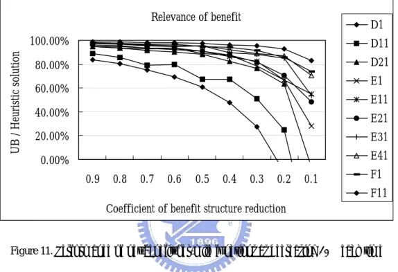
(7) List of Figures Figure 1. An MBCPP example............................................................................. 2 Figure 2. Cost and benefit structure...................................................................... 2 Figure 3. The OTP example network. .................................................................. 4 Figure 4. Set of qij + 1 parallel traversal links in Ga to replace (i, j). ........................ 5 Figure 5. Set of nodes converted from .................................................................. 5 Figure 6. The original nodes defined as complete sub-graph as Gb´. ....................... 7 Figure 7. A example of MBCPP with 4 nodes and 5 edges. ................................... 8 Figure 8. A MBCPP network use network transformation to OTP. ....................... 9 Figure 9. Flow chart for the modified Tsiligirides algorithm.................................15 Figure 10. The example that has ten arcs, ten nodes and three kinds of roads with depot is node 1 ......................................................................................16 Figure 11. Performance of net-benefit-per-mile functions as decreasing 10% each time ......................................................................................................17. vii.

(8) Notations G. ：MBCPP network with nodes set V, edges set E. V. ：A set of nodes. E. ：A set of edges. cijs. ：The service cost which traversal from node i to node j with service. cijd. ：The deadhead cost which traversal from node i to node j without service. qij. ：The number of expansion of edge (i, j) rij = 1,2,3,...qij + 1 (if qij > 0) = 1,2,3,...qij + 1 (if qij = 0). bijrij. ：A set of non-negative benefit which from node i to node j for the rij -th traversal with service. cij r. ：The net cost of the rij -th traversal of the edge (i, j). s (n). ：The score of control point (node). ij. GOP1 ：The Generalization of Orienteering Problem 1 is depot and termination node as the same, besides each node can be visited once GOP2 ：The Generalization of Orienteering Problem 2 is depot and termination node as the same without node visitation constraint GOP3 ：The Generalization of Orienteering Problem 3 is depot and termination node as distinct and each node can be visited once GOP4 ：The Generalization of Orienteering Problem 4 is depot and termination node as distinct without node visitation constraint Tmax. ：The total travel time of visiting a subset of nodes in V. ijrij. ：A set of parallel links with new score which replace each edge (i, j) in E. Ga. ：The expanded network. Gb. ：The converted network. Gb´. ：The converted network with advance connecting definitions. Gc. ：The resulting transformed network. viii.

(9) t. ：Travel time between node i to node j. si. ：duplicate node. T1. ：Modified Tsiligirides algorithm with one coordinate node. T2. ：Modified Tsiligirides algorithm with two coordinate nodes. T3. ：Modified Tsiligirides algorithm with three coordinate nodes. T4. ：Modified Tsiligirides algorithm with four coordinate nodes. T5. ：Modified Tsiligirides algorithm with five coordinate nodes. A(i ). ：Desirability of node. C. ：Distance from node i to node j. NPi. ：Normalize desirability value of coordinate nodes. i = 1, 2 , 3, … pi. Wi. ：Weighted measurement value. di. ：Summation of durations from node i to start node and end node. x. ：Weighted number. y. ：Weighted number. z. ：Weighted number. gi. ：The duration from center of gravity point to node i. L(i). ：Learning component. α. ：Scaling parameter. Di. ：Desirability measurement value. R. ：Random number. Pi. ：Probability value. ix.

(10) 1. Introduction The Chinese Postman Problem (CPP) is the problem of finding the shortest postman tour covering all roads in the network. There are various generalizations of the CPP. The CPP includes the Direct Chinese Postman Problem (DCPP) and the Mixed Chinese Postman Problem (MCPP) by Edmonds and Johnson (1973), the Windy Chinese Postman Problem (WCPP) by Minieka (1979), the Rural Postman Problem (RPP) by Christofides et al. (1981), the Capacitated Arc Routing Problem (CARP) by Golden and Wong (1981), the Hierarchical Postman Problem (HPP) by Dror (1987), the k-person Chinese Postman Problem (k-CPP) by Pearn (1994), and many others. The Maximum Benefit Chinese Postman Problem (MBCPP) is another interesting generalization of the CPP, in which each arc on the network is associated with a service cost for the traversal with service, a deadhead cost for the traversal with no service, and a set of benefits. Each time an arc is traversed then a benefit is generated. The objective of the MBCPP is to find a postman tour traversing a set of selected arcs with maximized total net benefit. Such a generalization reflects real-world situations more closely. Real-world applications related to the MBCPP include routing of solid waste collection vehicle, milk collecting trucks, snowplows, and salt spraying trucks. These applications had been formulated as traditional arc routing problems (such as CPP, RPP, CARP) in which only one single service traversal on each arc is considered. In real situations, however, the demand on the arc may require multiple service traversals to complete the service. It is true for most snowplow operations because one single traversal only can remove a portion of the snow on a street. Multiple service traversals are required, in this case, to complete the removal of snow. Assad and Golden (1995), Dror (2000), Eiselt et al. (1995a, 1995b), summarized the theory and applications of arc routing problems.. 2. Literature review. 2.1 Maximum Benefit Chinese Postman Problem The MBCPP was first introduced by Malandraki and Daskin (1993), in which the solution procedures for MBCPP on totally directed networks were investigated. In this paper, we consider MBCPP on totally undirected network. The MBCPP 1.

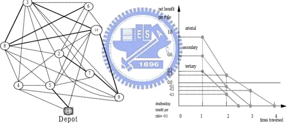
(11) may be briefly defined as follows. Let G = (V , E ) be a totally undirected network with V representing the set of nodes (cities), and E representing the set of edges (two-way streets). For each edge (i, j ) ∈ E , a non-negative service cost cijs for the traversal with service, and a non-negative deadhead cost cijd for the traversal with no service are given with cijs ≥ cijd . A set of non-negative benefits bijrij from node i to node j for the rij -th traversal is given, where rij = 1, 2,..., qij . For each edge (i, j ) ∈ E , the costs/benefits from node i to node j and node j to node i are set to be equivalent. To reflect real situations, we assume that bijrij is non-increasing in rij . Therefore the net cost of the rij -th traversal on the edge (i, j) can be expressed as cijrij = cijs − bijrij for rij = 1, 2,..., qij , where qij = max{rij | cijrij < cijd } . If rij ≥ qij + 1 , then the net cost is cijrij = cijd . That is, for the traversal of the deadhead edges, no benefit is generated. Then, the MBCPP is a kind of problem to find a postman tour, starting from the depot, traversing all edges in E, and returning to the same depot with minimized total net cost. 3. 6. net benefit per mile 10. arterial. 1.0. 8. secondary 2. 0.6. 4. tertiary. 0.3 0.2. 7. 0.0. 5. -0.1 -0.2 -0.3. 9. deadheading. 1. benefit per. D epot. mile= -0.5. Figure 1. An MBCPP example.. 0. 1. 2. 3. 4 times traversed. Figure 2. Cost and benefit structure.. The MBCPP has been shown to be more complex than the Traveling Salesman Problem (TSP). Malandraki and Daskin (1993) proposed a branch and bound algorithm with computation time growing exponentially, which only can solve small and moderate sizes of problems. Considering the example depicted in Figure 1 with ten nodes and thirty edges, node 1 represents the depot. Three types of edges (streets) considered include the arterial, the secondary, and the tertiary as shown in bold lines, thin line and dotted lines, respectively. Lengths of those streets are displayed in Table 1. Costs and benefits are defined to be proportional to the distance for each edge types, using the net-benefit-per-mile functions introduced by Malandraki and Daskin (1993), as depicted in Figure 2. The. 2.

(12) optimal solution of MBCPP for this example is (1, 4, 2, 7, 5, 1, 10, 5, 4, 8, 10, 9, 3, 2, 8, 6, 5, 8, 3, 10, 3, 7, 9, 7, 2, 10, 6, 3, 4, 9, 2, 6, 8, 9, 10, 8, 3, 5, 1) with total net benefit 75.6. Table 1. The edge lengths in the MBCPP example.. 1 2 3 4 5 6 7 8 9 10. 1. 2. 3. 4. 5. 6. 7. 8. 9. 10. — — — 3 5 — — — — 2. — — 3 2 — 2 5 3 3 3. — 3 — 3 3 2 3 5 3 5. 3 2 3 — 2 — — 3 2 —. 5 — 3 2 — 2 2 3 — 3. — 2 2 — 2 — — 5 — 2. — 5 3 — 2 — — — 5 —. — 3 5 3 3 5 — — 2 5. — 3 3 2 — — 5 2 — 5. 2 3 5 — 3 2 — 5 5 —. 2.2 Orienteering Tour Problem (OTP) The Orienteering Problem (OP), first investigated by Tsiligirides (1984), was referred to as a generalized traveling salesman problem (GTSP). Unlike the traveling salesman problem (TSP), the Orienteering Problem does not require to visit each node in V. If the OP involves both the number of control points with associated scores, especially s(1) = s(n) = 0, and that the starting node 1 is different from the ending node n, then it is termed as generalization orienteering problem. Ramesh et al. (1991) classified Orienteering Problem into four categories described as below. GOP1: In this version, node 1 and node n are identical. Consequently, the objective of the problem is to find a subtour of G starting and ending at node 1. GOP2: In this problem, GOP 2 is the same as GOP 1, but it allows of relax visitation of nodes in the subset. GOP3: In this version, node 1 and node n are different. Therefore, the problem turns to find a path starting from node 1 and returning to the ending node n. Further, each node in the path is visited only once. GOP4: This problem is similar to GOP3, but it allows of relax visitation of nodes in the subset. Thus, it is a relaxation of GOP3. In the following, we present a simple network transformation, which converts 3.

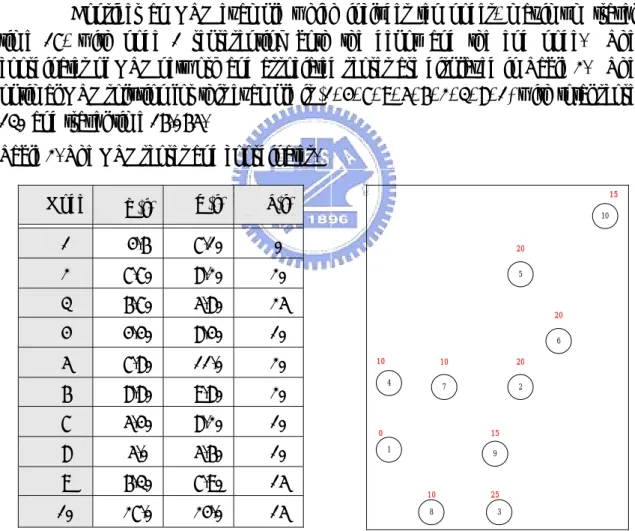
(13) the totally undirected MBCPP into the Orienteering Tour Problem, belonging to GOP2. The GOP2 may be briefly stated as follow. Given a complete network G with n nodes, each node is associated with a score s(i) ≥ 0 and with relax visitation of nodes in the visited subset. Between node i and node j, the travel time is pre-assumed to in V. The GOP2 turns to be a problem to find a closed tour visiting a subset of the nodes in V with maximized total score, while the travel time incurred is not greater than a predetermined value, Tmax. In MBCPP, the net cost is defined as cijrij = cijs − bijrij . Therefore, a negative cost cijrij is as well as positive benefit. In this paper, it is reasonable to focus on GOP2 with relaxation score constraint. OTP Example Consider an OTP example which includes ten nodes, maximum travel time 17, with node 1 representing both the depot and the end node. The coordinates of OTP network and associated scores are displayed in Table 2. The optimal OTP solution for this example is (1, 4, 7, 9, 5, 6, 2, 3, 8, 1) with total score 130 and travel time 16.065. Table 2. The OTP scores and coordinates. Node. X(i). Y(i). S(i). 1. 4.6. 7.10. 0. 2. 7.70. 8.20. 20. 3. 6.70. 5.80. 25. 4. 4.40. 8.40. 10. 5. 7.80. 11.0. 20. 6. 8.80. 9.80. 20. 7. 5.40. 8.20. 10. 8. 5.0. 5.60. 10. 9. 6.30. 7.90. 15. 10. 27.0. 24.0. 15. 15 10. 20 5. 20 6 10 4. 0. 10. 20. 7. 2. 15 1. 9. 10. 25. 8. 3. Figure 3. The OTP example network. Both the OP and the OTP are NP-hard problems, which have received extensive research attentions. Research papers focused on the OP and OTP including Tsiligirides (1984), Golden et al. (1987), Golden et al. (1988), Keller (1989), Ramesh and Brown (1991), Ramesh et al. (1992), Leifer and Rosenwein 4.

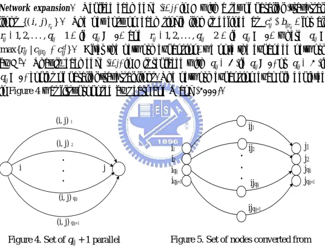
(14) (1994), Wang et al. (1995), Chao et al. (1996), and Tasgetiren and Smith (2000). In the following, we present a simple transformation which converts the MBCPP into a special class of the Orienteering Tour Problem (OTP). Consequently, the existing heuristics for OP and OTP may be applied to solve the MBCPP approximately.. 3. Transforming MBCPP into OTP. 3.1 Defining the transformation Network expansion. Replace each edge (i, j) in E with a set of parallel (traversal) links {( i , j ) rij } . The net cost on each single link is defined as cijs − bijrij , for all. rij = 1, 2, . . . , qij + 1 , if qij > 0, and rij = 1, 2, . . . , qij + 2 , if qij = 0, where qij = max{rij | cijrij < cijd } . After the network expansion, we note the expanded network by Ga. That is, each edge (i, j) in E is replaced with qij + 1 (if qij > 0) or qij + 2 (if qij = 0) copies of parallel traversal links. The network expansion example depicted in Figure 4 was first proposed by Pearn and Wang (2000). (i, j) 1. ij1. (i, j) 2 i. . . .. i1 i2 iqij iqij+1. j. . . .. ij2. ijqij. j1 j2 jqij jqij+1. (i, j) qij. ijqij+1 (i, j) qij+1. Figure 5. Set of nodes converted from the qij + 1 parallel traversal links.. Figure 4. Set of qij + 1 parallel traversal links in Ga to replace (i, j).. Network conversion. Replace each traversal link (i, j ) rij in Ga with a new node ij rij connecting to the nodes i and j ; replace each node i with pi copies of duplicated nodes, where pi = ∑ j ( qij + 1)| qij > 0 + ∑ j ( qij + 2)| qij = 0 , to obtain the converted network, noted by Gb, consisting of the set of nodes { i si | i ∈ V } ∪ { ij rij | (i, j ) ∈ E } , where { isi | si = 1, 2, . . . , pi }. Connecting duplicate nodes. The original nodes can be transformed into a complete sub-graph Gb´. Each edge (i, j) in E has a number of pi copies of duplicated nodes, strongly connected in Gb´ depicted in Figure 6, where pi = {∑ j ( qij + 1)| qij > 0 + ∑ j 5.

(15) ( qij + 2)| qij = 0 }. Clearly, the original nodes in V are discarded and replaced by new node ij rij and isi . The duplicate nodes also have directed links to each other in original nodes. Score setting. On the converted network, Gb´, set the score on node isi as s( isi ) = 0 for all pi copies of the duplicated nodes in { isi | i ∈V } . Also set the score on the new node ij rij as s( ij rij ) = cijs − bijrij for all qij copies of the (converted) new nodes, and s( ijrij ) = cijd for the other one/two (converted) new nodes with rij = qij + 1, and rij = qij + 2. Travel time setting. On the converted network Gb´, the travel time between the duplicated nodes is defined as t ( ij rij , isi ) = t ( j s j , ij rij ) = 1, where si = 1, 2, . . . , pi , and the new node ij rij is converted from the parallel traversal links with rij = 1, 2, . . . , qij + 1 (or qij + 2). The travel time between other pairs of nodes is defined as ∞. In the set of duplicate node isi , the travel time is define as t ( isi , isi+1 ) = t ( js j , js j +1 ) = 0. The time constraint, Tmax , is set to ∑ (i, j)∈E 2 ( qij + 2). The transformed network with node score and inter-node traveling time is defined as above noted by Gc. Traversal rules. Traversal rule 1 is that only two duplicate nodes should be visited from the last control point inserted to the route to the next candidate for control point. Clearly, if we traverse more than two duplicate nodes successively twice at the same time, the solution of MBCPP will be infeasible. Then, travel time is define as ∞. Traversal rule 2 is that the traveling sequence depends on whether the control point ijrij with maximum score is visited or not in the network Gc. The control point variation. In MBCPP, each link from node i to node j after network expansion and conversion can be illustrated in Figure 4 and Figure 5 by Pearn and Wang (2000). The origin node only connects each edge in E. The link (i, j) with a set of new control points ijrij with scores are generated when we traverse the link (i, j) each time. We use duplicate node ijrij to express control points associated with scores which satisfy the GOP2 conditions. Therefore, we can easily and exactly transform MBCPP into GOP2 so as to solve it by OP algorithms.. 6.

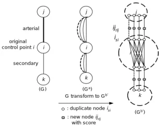
(16) j. j. ij rij. arterial original control point i. j. isi i. i. i secondary k. k. (G). (G a ) G transform to G b' : duplicate node isi. k (G b'). : new node ij rij with score. Figure 6. The original nodes defined as complete sub-graph as Gb´. 3.2 Steps to transformation The Maximum Benefit Chinese Postman Problem (MBCPP) can be transformed to the Orienteering Tour Problem (OTP) as follow: Step 1: Construct an initial MBCPP graph for the corresponding Orienteering Tour Problem by setting G. Step 2:. Replace each edge (i, j) in E with a set of parallel links {(i, j) r } as graph ij. Ga. Step 3:. Replace each links {(i, j) r } in Ga with a new node ijrij ij. { i si | i ∈ V } ∪ { ij rij | (i, j ) ∈ E } , where { isi | si = 1, 2, . . . , pi } as graph Gb.. Step 4: On the converted network Gb, transform the original node to sub-network and define that they are strongly connected. In the sub-network, each arc from duplicate node isi to isi +1 is directed. Then Gb is transformed to Gb´ Step 5: cijrij. Set the score on the new node as s( ijrij ) = cijs − bijrij in Gb´.. cijs − bijrij , if rij = 1,2,...., qij = d , if rij = qij + 1 |qij > 0 or rij = qij + 2 |qij = 0 cij. Step 6: Set the travel time between the duplicate nodes as follows. Gc denotes the resulting network after travel time setting. t (isi , ijrij ) = t (ijrij , jsi ) = 1 t (isi , isi+1 ) = t ( js j , js j +1 ) = 0. Tmax = ∑ (i, j)∈E 2 ( qij + 2 ). 7.

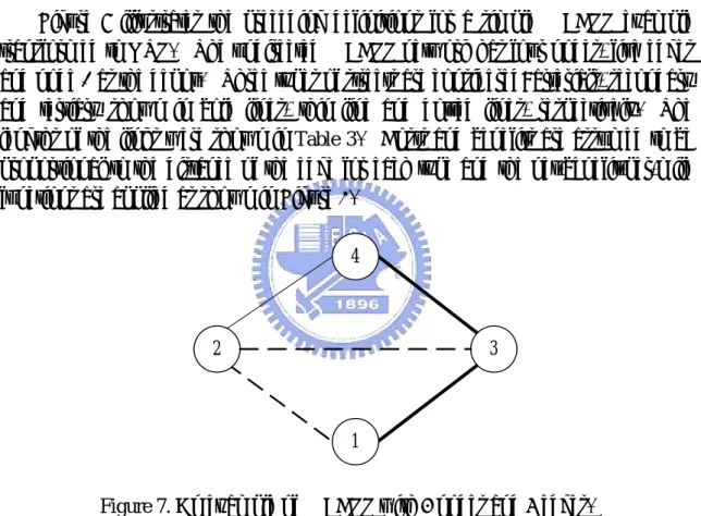
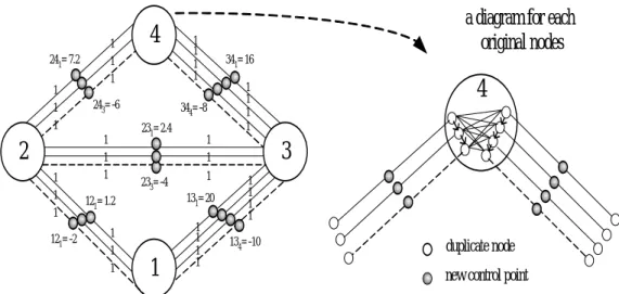
(17) Theorem: The optimal OP solution over the transformed network Gc, is equivalent to that over the original network G(V, E) for MBCPP. For edges with qij > 0, the number of traversals on a specific link with no service is not greater than one. If not, then remove two copies of such traversal links (with deadhead cost) and increase the total net benefit. Further, if removing two such traversal links can not separate the remaining network into disconnected components, then the solution remains feasible. 3.3. An example for transforming MBCPP to OTP Figure 7 illustrates the preceding definitions for a simple MBCPP example transformed to OTP. The undirected MBCPP network has four nodes, five edges and node 1 as the depot. Three types of streets are considered: arterials, secondary and tertiary shown in bold lines, thin line and dotted lines, respectively. The lengths of the links were shown in Table 3. Costs and benefits are assumed to be proportional to the distance of the edge for each type and the net-benefit-per-mile functions are applied as shown in Figure 2.. 4. 2. 3. 1 Figure 7. An example of MBCPP with 4 nodes and 5 edges. Table 3. The length of edge (i, j) from node i to node j. Edges 1 2 3 4. 1 — 4 20 —. 2 4 — 8 12. 3 20 8 — 16. 4 — 12 16 —. The undirected network G of MBCPP is transformed to a corresponding OTP network diagram as shown in Figure 8 below.. 8.

(18) 1 1 1. 241= 7.2 1 1 1. 4. 243= -6. 2 1 1 1. 1 131= 20. 1 1 1. 1. 1 1 1 1. 4. 1 1 1 1. 1 1. 233= -4. 121= 1.2. 121= -2. 341= 16. 344= -8 231= 2.4. 1 1 1. a diagramfor each original nodes. 1 1 1 1. 3 1 1 1 1 134= -10. duplicate node newcontrol point. Figure 8. A MBCPP network use network transformation to OTP.. 4. Orienteering Problem (OP) algorithms The OP algorithms usually fall into two classifications: exact approaches including Ramesh et al. (1992) and Pillai (1992), and heuristic solution procedures such as Tsiligirides (1984), Golden et al (1987, 1988), Keller (1989), Ramesh (1991), Wang et al. (1995), Chao et al. (1996), Tasgetiren and Smith (2000). We briefly review these algorithms as bellow. 4.1 Tsiligirides Algorithm (1984) Tsiligirides first proposed two heuristics for the Orienteering Problem. One is a stochastic algorithm and the other is a deterministic one. The stochastic algorithm is based on Monte Carlo method to generate a large number of routes, and then select the best one among them. Tsiligirides algorithm evaluates each control point i by the measurement A ( i ) = { S i / C ( last , i )} 4 . If there are less than four nodes, then they need to be normalized by using NPi = Ai / ∑ qk =1 Ak . From the candidate nodes, select a node inserted to the route by generating a random number between 0 and 1. The procedure is iterating until Tmax can’t be added any duration from the last node added to next candidate node.. Another heuristic is a. deterministic algorithm based upon vehicle scheduling method proposed by Wren and Holiday (1972). The deterministic algorithm, without using random numbers and probabilities divides the search area into sectors by using two concentric circles. 9.

(19) and a known arc length. In order to add new nodes, the sectors are changed by varying the two radii of the circles and spinning arc length. Routes construction procedure stops when all nodes in particular sector, which has been visited or any duration added to the current route will violate the rule for Tmax. 4.2 Golden, Levy and Vohra Algorithm (1987) Golden et al. in 1987 proposed a heuristic containing three steps: route construction, route improvement and a new concept center of gravity. Route construction uses weighted measurement Wi = x ⋅ Si + y ⋅ g i + z ⋅ d i to assess each node, where Si is the score of node i, gi is duration from center of gravity point to node i, d i is summation of durations from node i to starting node and ending node, and the sum of the weighted numbers x, y and z is unity. In route improvement, Golden et al. used 2-opt method to decrease current Tmax value. The center of gravity is the heuristic spirit. The new center of gravity is continuously generated by combining step1 and 2 to increase total score without violate Tmax. The procedure is repeated until the path with highest objective value appears again then the procedure stops. 4.3 Golden, Wang and Liu Algorithm (1988) Golden et al. (1988) introduced subgravity algorithm which includes learning and randomness concepts. The former is developed from Tsiligirides’s stochastic algorithm, and the latter is a key factor to result better solution. This is because that route construction uses weighted measurement Wi = x ⋅ Si + y ⋅ g i + z ⋅ d i and the. The learning component contains adjusted information. We formulate L(i) as learning measurement. According to variation of L(i) to adjust Si, gi and di values. The initial L(i) is equal to one. If node i associates with path score higher than total average scores, then L(i) > 1 and node i is reward or else L(i) < 1 and node is penalized. For each center of gravity of five squares in graph, total 100 solutions are generated and the best solution is selected as result. 4.4 Keller Algorithm (1989) Keller (1989) revised his multi-objective vending problem’s algorithm to solve OP. The algorithm consists of 2 stages: route construction and route improvement. At the route construction stage, first computes the desirability of each node i. For each node not belonging to the current route, we select the one with the largest. 10.

(20) desirability merit for insertion to the route. At the second stage, first removes one node then inset none; one or two nodes into the route in order to increase total score. Next, remove identification of nodes clusters and inset another identification of node clusters to increase total score. 4.5 Ramesh and Brown Algorithm (1991) The algorithm includes four steps that are node insertion, length improvement, node deletion and maximal insertion. In node insertion, relaxes T value limit to construct initial route. The length improvement to uses 2-opt and 3-opt to decrease Tmax value. The node deletion is similar to Kell (1989) route improvement step two. One node is removed and then another node is inset to decrease current T value. The maximal insertion tries to increase the total score by a new node i that is not on the current route. 4.6 Ramesh, Yoon and Karwan Algorithm (1992) Ramesh et al. (1992) developed an optimal solution procedure, which uses Lagrangean relaxation within a branch and bound technique. The Lagrangean relaxation is solved by a degree-restricted spanning tree manner. The algorithm contains six steps: (1) initialization, (2) scaling parameter α , (3) upper & lower bounding, (4) branching rule, (5) upper bounding, (6) measuring and backtracking. The computational results show that the algorithm can be processed to solve the medium and large size problem. 4.7 Pillai Algorithm (1992) The Pillai algorithm claimed that the final solution is optimal. The algorithm is based on branch and cut technique to solve the problem. Consequently, it only can be employed on small or moderate size problems. The Pillai algorithm first applies a relaxed linear programming with no violated constraints. If the solution is a non-integer, then construct a feasible solution by employing branch and cut method to find the optimal solution; otherwise, then the procedure is stopped. 4.8 Leifer and Rosenwein Algorithm (1994) Leifer and Rosenwein (1994) first defined a 0 － 1 integer programming formulation for the Orienteering Problem, then use bound procedure by adding constraints and valid inequalities to solve three successive the linear problems. 11.

(21) The algorithm is to find a tight upper bound for the optimal objective function value. 4.9 Wang et al. algorithm (1995) In Wang et al. algorithm, the neural network applies two-dimensional cell as the tight bound and the energy function with fourth order convex function to solve OP approximately. 4.10 Chao, Golden and Wasil Algorithm (1996) Chao et al. (1996) algorithm consists of two stages: stage one is initialization using greed criterion to inserted node to the route. The rule of insertion is to select a node with cheapest insertion cost while its score is ignored. The second stage is improvement including two-point exchange, one-point movement, clean-up and reinitialization. Two-point exchange is that one new point moves in and one point moves out, if total score increases and current time doesn’t violate the Tmax. One-point movement is to insert a new node, if total score increases and route is feasible. Clean-up step is to apply 2-opt to improve Tmax , at which the algorithm has more opportunities to insert nodes. Finally, remove the nodes with smallest measurement ratio from the route and redo improvement stage. 4.11 Tasgetiren and Smith algorithm (2000) Tasgetiren and Smith algorithm (2000) is one kind of genetic algorithm, of which the performance is the same with Chao et al. (1996). Both outperformed other heuristics of OP. The algorithm first employs node omission probability based on Tmax length constraint to generate some feasible path, then applies crossover operator and local search mutation to improve the initial path. Until a rear-optimally solution is found. But the computational time of the algorithm is longer.. 5. Modified Tsiligirides Algorithm Here we apply the Tsiligirides’s algorithm to solve the new network after transforming MBCPP to OTP. The new OTP network is different from the OTP introduced by Ramesh et al. (1991). Because our OTP is not a complete network which has the relaxation of score constraint. But it is more close to real world 12.

(22) situations and easily transformed to MBCPP. Furthermore, we can input real urban street map formulated to MBCPP which can be transformed to OTP, and solved by modified Tsiligirides algorithm. Since the MBCPP can be easily transform to OTP, the Tsiligirides’s algorithm should be modified in order to solve the new OTP. We note that desirability measurement may be revised to n D i = S i / ∑ k =1 S k , n = 1, 2, . . ., q. Note that the travel time is defined as t ( ij rij , isi ) = t ( j s j , ij rij ) = 1, between the duplicated node Si = 1, 2, . . . , pi . Neither the distance from node i to node j is an important factor now, nor the travel time. The improvement method of Tsiligirides’s algorithm is not needed in our modified algorithm. The objective function of OTP increases score while a new node is inserted. Obviously, without increasing any score or decreasing the total score, a new node is not allowed to insert. In MBCPP applications, the objective is to seek a postman tour with maximized total benefits. In snowplow operations, a street somehow must be served more than once, because the benefit of link (i ,j) is positive and smaller than service cost, but still better than deadhead cost for objective function. The point is that Tsiligirides algorithm can’t handle negative score of node. We translate the negative score to a positive one and measure it by Di = Si 4 / ∑k =1 S k . A random number R ∈ U (0,1) ranged between 0 and 1 is generated. The candidate node i is randomly selected with probability Pi as a new node inset to the current route. Nodes continuously are added to the current route until each edge (street) in E is served at least once. Then, apply the shortest path method from last node on the route back to the depot. The procedure is iterated until 400 routes are generated and a route with highest score is selected as the finally solution. The flow chart in Figure 9 provides an easy way to understand the sequence of logical operations of the modified Tsiligirides algorithm. The bottleneck of the modified Tsiligirides algorithm is the shortest path segment which requires an order of O(n3) computations. Therefore, the complexity of modified Tsiligirides algorithm is O(n3).. 6. Computational results. 6.1 Modified Tsiligirides algorithm performance To test and verify the proposed solution procedures, we generate six sets of test problems, which are randomly generated with the following characteristics described in Table 4.. 13.

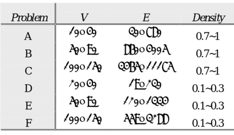
(23) Table 4. Characteristics of six sets of 210 problems. Problem A. V 10~40. E 30~780. Density. B. 50~90. 860~4005. 0.7~1. C. 100~150. 3465~11175. 0.7~1. D. 20~40. 19~230. 0.1~0.3. E. 50~90. 120~1334. 0.1~0.3. F. 100~150. 559~3288. 0.1~0.3. 0.7~1. V = number of nodes; E = number of edges The details of each set of test problems were described in Table 10 on appendix B. Costs and benefits are assumed to be proportional to the distance of each edge with the net-benefit-per-mile function introduced by Malandraki and Daskin (1993). The problems A to C are dense, while D, E and F are sparse. We also compute average ratios to the upper bound of 210 problems due to their complexity. The modified Tsiligirides algorithm was coded in Visual Basic 6.0 and implemented on Pentium IV personal computer with CPU 2.4G and 512M memories. Start. Yes All edges in network are serviced at least once ?. No. Yes. Does all of candidate nodes associate with score s(i) < 0 ?. No Perform shortest path method, back to the Depot Compute "desirability" and randomly select a candidate node inserted to the current route. Translate the candidate score then compute "desirability" and randomly select one node from four candidate nodes. Terminate. 14.

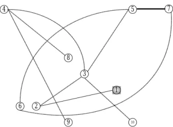
(24) Figure 9. Flow chart for the modified Tsiligirides algorithm The modified Tsiligirides algorithm has five variations, which have different numbers of candidate nodes, noted by T1, T2, T3, T4 and T5. For instance, T1 has one candidate node, T2 has two candidate nodes, and so on. The comparisons of the performances of T1, T2, T3, T4 and T5 on the 210 test problems are summarized in Table 7, Table 8 and Table 9. The average ratio to the upper bound, the worst ratio to the upper bound, the number of best solutions obtained, and the number of worst solutions obtained are recorded. The networks of Table 7(a), Table 7(b) and Table 7(c) are dense. Since T5 achieved 42 best solutions in problem set A, B and C, it seems to be the best algorithm for dense networks. Out of the sparse networks shown in Table 7(d), Table 7(e) and Table (f), T2 achieved 30 best solutions, while T4 and T5 gained 24 best solutions and 23 best solutions, respectively. In the comparison of the average ratio to the upper bound between T2, T4 and T5 among problem set D, E and F, T2 reached 98.35% and T4 gained 98.38%, while T5 achieved up to 98.40%. Therefore, T5 is the best choice out of 5 variations of modified Tsiligirides algorithm no matter whether the network is dense or sparse. The modified Tsiligirides algorithm is based on inserting a randomly selected candidate node into the route. Therefore, if the number of run times increases, then the solution is near to the optimal one. In fact, the solution will not increase without limits. In Table 9(e), we varied the number of run times from 100 to 400 times. T5 is the best one of all algorithms when R = 100, 200, 300 and 400, since the average ratios to the upper bound for T5 are 99.008%, 99.079%, 99.1% and 99.122%, respectively. Obviously, when the number of run times increases, the average ratio to the upper bound goes up slightly. Out of 210 test problems, 65 solutions are the best for R = 100 as shown in Table 9(e). When R= 200 or 300, there are 49 best solutions and 96 worst ones. However, the numbers of the best and the worst solutions are approximately equal when the run times are 400. In fact, the 96 worst solutions were very close to improvement solutions out of 400 run times. 6.2 Benefit structure analysis To investigate coefficient of benefit structure in MBCPP, considered the MBCPP network depicted in Figure 10 with symmetric cost functions produced from the Cartesian coordinates in Table 5, net-benefit-per-mile functions and three kinds of roads the same as example 1 of MBCPP.. 15.

(25) 4. 7. 5. 8. 3. 1 6. 2. 9. 10. Figure 10. The example that has ten arcs, ten nodes and three kinds of roads with depot is node 1 Table 5. The Cartesian coordinates for the MBCPP pathological example.. Node 1 2 3 4 5 6 7 8 9 10. X(i) 73 24 52 0 87 7 90 46 47 86. Y(i) 36 2 47 85 83 20 81 57 13 9. The network density of the pathological example is 0.2, which belongs to sparse network. It has an upper bound 241.746. The branch and bound method was solved the pathological example to obtain an optimal solution 120.64, and the optimal ratio to the upper bound near to 50%. The optimal route of the MBCPP is 1-2-3-10-3-5-7-6-5-7-5-3-4-8-4-9-4-3-2-1. Also, we applied the T5 of modified Tsiligirides algorithm to find the optimal solution 120.64 within five run times for this example. In addition, the route was obtained 1-2-3-10-3-5-7-6-5-7-53-4-8-4-9-4-3-2-1 for the T5 of modified Tsiligirides algorithm. Therefore, the modified Tsiligirides algorithm can be applying in the MBCPP which was after network transformation. To investigate the impact of the benefit structure on the solutions of T5 algorithm, we decreased the net-benefit-per-mile functions by 10% each time, and verified 10 test problems from problem set D, E, and F (sparse networks), including D1, D11, D21, E1, E11, E21, E31, E41, F1 and F11. The results showed that the performance of net-benefit-per-mile functions decreased 16.

(26) while coefficient of benefit structure was reduced, as depicted in Figure 11 and recorded in Table 6. Obviously, T5 algorithm performs well for dense or large size networks. We point out that the net-benefit-per-mile function is an important factor for our modified Tsiligirides algorithm. If sparse and small networks have low coefficient (0.3 ~ 0.1) of benefit structure, then the solution procedure could produce solutions of poor quality.. UB / Heuristic solution. Relevance of benefit. D1. 100.00%. D11. 80.00%. D21 E1. 60.00%. E11. 40.00%. E21. 20.00%. E31. 0.00%. E41. 0.9. 0.8. 0.7. 0.6. 0.5. 0.4. 0.3. 0.2. F1. 0.1. F11. Coefficient of benefit structure reduction. Figure 11. Performance of net-benefit-per-mile functions as decreasing 10% each time Table 6. The results of sparse network with reduce 10% coefficient of benefit each times. D1. 0.9. 0.8. 0.7. 0.6. 0.5. 0.4. 0.3. 0.2. 0.1. Best sol.. 407.045. 345.954. 284.862. 224.188. 163.734. 103.280. 44.457. -11.101. -68.691. UB. 485.573. 431.621. 377.668. 323.715. 269.763. 215.810. 161.858. 107.905. 53.953. Ratio. 83.83%. 80.15%. 75.43%. 69.25%. 60.70%. 47.86%. 27.47%. -10.29%. -127.32% -100.009. D11 Best sol.. 1134.797. 970.827. 785.400. 678.211. 477.343. 381.803. 215.338. 69.878. UB. 1273.084. 1131.630. 990.171. 848.723. 707.265. 565.815. 424.361. 282.906. 141.454. Ratio. 89.14%. 85.79%. 79.32%. 79.91%. 67.49%. 67.48%. 50.74%. 24.70%. -70.70%. D21 Best sol.. 2269.629. 1988.850. 1703.564. 1434.424. 1170.003. 875.208. 609.173. 336.962. -17.677. UB. 2390.735. 2125.098. 1859.459. 1593.824. 1328.185. 1062.548. 796.912. 531.274. 265.637. Ratio. 94.93%. 93.59%. 91.62%. 90.00%. 88.09%. 82.37%. 76.44%. 63.43%. -6.65%. E1 Best sol.. 2889.330. 2538.229. 2198.138. 1897.316. 1507.595. 1189.161. 797.915. 453.843. 95.033. UB. 3054.513. 2715.123. 2375.730. 2036.342. 1696.950. 1357.560. 1018.171. 678.780. 339.390. Ratio. 94.59%. 93.48%. 92.52%. 93.17%. 88.84%. 87.60%. 78.37%. 66.86%. 28.00%. Best sol.. 6127.019. 5433.122. 4693.601. 3975.813. 3248.827. 2471.900. 1772.732. 956.046. 393.466. UB. 6452.262. 5735.344. 5018.419. 4301.508. 3584.585. 2867.668. 2150.754. 1433.834. 716.918. Ratio. 94.96%. 94.73%. 93.53%. 92.43%. 90.63%. 86.20%. 82.42%. 66.68%. 54.88%. E11. E21 Best sol.. 7242.989. 6382.623. 5473.091. 4690.783. 3801.397. 2923.253. 2042.630. 1179.815. 403.954. UB. 7528.877. 6692.335. 5855.787. 5019.251. 4182.705. 3346.164. 2509.626. 1673.082. 836.542. 17.

(27) 95.37%. 93.46%. 93.46%. 90.88%. 87.36%. 81.39%. 70.52%. Best sol. 10547.249. 9308.129. 8065.303. 6868.281. 5744.037. 4311.264. 3184.760. 2043.656. 643.973. UB. 10834.319. 9630.506. 8426.691. 7222.879. 6019.065. 4815.252. 3611.440. 2407.626. 1203.813. Ratio. 97.35%. 96.65%. 95.71%. 95.09%. 95.43%. 89.53%. 88.19%. 84.88%. 53.49%. Best sol. 12426.788. 10949.028. 9530.659. 8094.778. 6722.719. 5191.226. 3760.000. 2452.508. 999.352. UB. 12717.436. 11304.388. 9891.336. 8478.291. 7065.240. 5652.192. 4239.145. 2826.096. 1413.048. Ratio. 97.71%. 96.86%. 96.35%. 95.48%. 95.15%. 91.84%. 88.70%. 86.78%. 70.72%. Best sol. 17321.913. 15306.686. 13341.553. 11361.702. 9309.869. 7393.545. 5385.887. 3373.817. 1448.918. UB. 17677.764. 15713.568. 13749.372. 11785.176. 9820.975. 7856.780. 5892.588. 3928.390. 1964.196. Ratio. 97.99%. 97.41%. 97.03%. 96.41%. 94.80%. 94.10%. 91.40%. 85.88%. 73.77%. Best sol. 37777.108. 33500.228. 29180.155. 24931.678. 20677.240. 16335.981. 12119.757. 7889.587. 3524.952. UB. 38163.471. 33923.085. 29682.695. 25442.314. 21201.925. 16961.540. 12721.157. 8480.770. 4240.386. Ratio. 98.99%. 98.75%. 98.31%. 97.99%. 97.53%. 96.31%. 95.27%. 93.03%. 83.13%. Ratio. 96.20%. 48.29%. E31. E41. F1. F11. 7. Conclusion The Maximum Benefit Chinese Postman Problem (MBCPP) is a practical generalization of the well-known Chinese Postman Problem (CPP), which has many applications. In this paper, we proposed a simple network transformation which converts the MBCPP to OTP and modified Tsiligirides algorithm to solve the MBCPP near-optimally. The modified Tsiligirides algorithm has five variations that are T1, T2, T3, T4 and T5. The result indicates that T5 is the best criteria of the modified Tsiligirides algorithm. Furthermore, we investigated net-benefit-per-mile effect on modified Tsiligirides algorithm. For low coefficient of benefit structure (0.3~0.1), the results showed that the modified Tsiligirides algorithm produced poor quality solutions on small and sparse networks. In other words, the proposed algorithm performs well on dense networks or sparse networks with net-benefit-per-mile at least 70﹪coefficient benefit structure considered in Malandraki and Daskin (1993). Others OP solution procedures also can be applied on the transformed MBCPP network, but the performances of them need further investigation.. 18.

(28) References Assad, A. and Golden, B. (1995). “Arc routing methods and applications.” Network Routing Handbooks in OR & MS, Vol. 8, Elsevier Science. Ball and Magazine (1988). “Sequencing of insertion in printed circuit board manufacturing.” Operations Research, 36(2), 192-201. Chao, I. M., Golden, B. L. and Wasil, E. A. (1996). “A fast and effective heuristic for the orienteering problem.” European Journal of Operations Research, 88, 475-489. Christofides, N., Campos, V., Corberan, A. and Mota, E. (1981). “An algorithm for the rural postman problem.” Imperial College Report IC-OR. Dror, M., Stern, H. and Trudeau, P. (1987). “Postman tour on a graph with precedence relation on arcs.” Networks, 17, 283-294. Dror, M. (2000). Arc Routing. Theory, Solutions and Applications. Kluwer Academic Publishers, Boston. Edmonds, J. (1967). “Optimum Branchings.” J. Res. Nat. Bur. Stand. 71B, 233-240. Edmonds, J. and Johnson, E. (1973). “Matching, Euler tour, and the Chinese postman problem.” Math. Programming, 5, 88-124. Eiselt, HA. Gendgreau, M. and Laporte, G. (1995a). “Arc routing problems, part 1: the Chinese postman problem.” Operations Research, 43, 231-242. Eiselt, HA. Gendgreau, M. and Laporte, G. (1995b). “Arc routing problems, part 2: the rural postman problem.” Operations Research, 43, 399-414. Golden, B. and Wong, R. (1981). “Capacitated arc routing problems.” Networks, 11, 305-315. Golden, B., Levy, L. and Vohra, R. (1987). “The orienteering problem.” Naval Research Logistics, 34(3), 307-318. Golden, B., Wang, Q. W. and Liu, L. (1988). “A multifaceted heuristic for the orienteering problem.” Naval Research Logistics, 35, 359-366. Keller, C. P. (1989). “Algorithms to solve the orienteering problem: a comparison.” European Journal of Operations Research, 42, 224-231. Leifer, A. C. and Rosenwein, M. B. (1994). “Strong linear programming relaxation for the orienteering problem.” European Journal of Operations Research, 73, 517-523. Minieka, E. (1979). “The Chinese postman problem for mixed network.” Management Science, 25, 643-648. Malandraki, C. and Daskin, M. S. (1993). “The maximum benefit Chinese postman problem and the maximum benefit traveling salesman problem.” European Journal of Operational Research, 65, 218-234. Pearn, W. L. (1994). “Solvable cases of the k-person Chinese postman problem.” Operations Research Letters, 16, 241-244.. 19.

(29) Pearn, W. L. and Wang, K. H. (2000). “On the maximum benefit Chinese postman problem.” Working paper, Department of Industrial Engineering and Management, National Chiao Tung University. Pillai, R. S. (1992). The traveling salesman subset-tour problem with one additional constraint (TSSP+1). Ph.D. Dissertation, The University of Tennessee, Knoxville, TN. Ramesh, R. and Brown, K. M. (1991). “An efficient four phase heuristic for the generalized orienteering problem.” Computers ＆ Operations Research, 18(2), 151-165. Ramesh, R., Yoon, Y. S. and Karwan, M. H. (1992). “An optimal algorithm for the orienteering tour problem.” ORSA Journal on Computing, 4(2), 155-165. Tasgetiren, M. F. and Smith, A. E. (2000). “A genetic algorithm for the orienteering problem.” Proceedings of the 2000 congress on Evolutionary Computation, San Diego, CA, 1190-1195. Tsiligirides, T. (1984). “Heuristic methods applied to orienteering.” Journal of the Operations Research Society, 35(9), 797-809. Wang, Q., Sun, X., Golden, B. and Jia, J. (1995). “Using artificial neural networks to solve the orienteering problem.” Annals of operations research, 61, 111-120. Wren, A. and Holiday, A. (1972). “Computer scheduling of vehicles from one or more depot to a number of delivery points.” Operations Research Quarterly, 23, 333-344.. 20.

(30) Appendix. Table 7(b). Performance comparisons of T1, T2, T3, T4 and T5 on problem set B1-B50 (dense networks, R = 400). T1 T5 T2 T3 T4. Appendix A Performance comparisons among T1~T5. Average ratio to the upper bound (%) Worst ratio to the upper bound (%) Number of best solution obtained Number of worst solution obtained Average run time in CPU seconds. Table 7(a). Performance comparisons of T1, T2, T3, T4 and T5 on problem set A1-A40 (dense networks, R = 400). T1 Average ratio to the upper bound (%) Worst ratio to the upper bound (%) Number of best solution obtained Number of worst solution obtained Average run time in CPU seconds. T2. T3. T4. T5. 99.315. 99.54. 99.551. 99.545. 99.556. 96.898. 98.058. 98.058. 98.058. 98.058. 2. 9. 20. 15. 18. 34. 1. 4. 0. 0. 26.7. 26.7. 26.7. 26.7. 26.7. 99.875. 99.903. 99.901. 99.907. 99.907. 99.809. 99.842. 99.831. 99.843. 99.813. 1. 10. 4. 17. 18. 41. 4. 2. 1. 2. 513.62. 513.62. 298.86. 307.19. 308.32. Table 7(c). Performance comparisons of T1, T2, T3, T4 and T5 on problem set C1-C20 (dense networks, R = 400). T1 T5 T2 T3 T4 Average ratio to the upper bound (%) Worst ratio to the upper bound (%) Number of best solution obtained Number of worst solution obtained Average run time in CPU seconds. 21. 99.93. 99.939. 99.946. 99.946. 99.947. 99.844. 99.883. 99.89. 99.894. 99.919. 0. 2. 7. 5. 6. 14. 4. 0. 1. 1. 2074.86. 2096.38. 2097.67. 2084.63. 2085.97.

(31) Table 7(f). Performance comparisons of T1, T2, T3, T4 and T5 on problem set F1-F20 (sparse networks, R = 400). T1 T5 T2 T3 T4. Table 7(d). Performance comparisons of T1, T2, T3, T4 and T5 on problem set D1-D30 (sparse networks, R= 400). T1 T5 T2 T3 T4 Average ratio to the upper bound (%) Worst ratio to the upper bound (%) Number of best solution obtained Number of worst solution obtained Average run time in CPU seconds. 96.236. 96.929. 96.946. 97.03. 97.069. 86.769. 86.769. 86.769. 86.769. 86.769. 2. 12. 6. 8. 8. 17. 4. 2. 5. 1. 10.35. 10.35. 10.57. 10.58. 10.5. Average ratio to the upper bound (%) Worst ratio to the upper bound (%) Number of best solution obtained Number of worst solution obtained Average run time in CPU seconds. Table 7(e). Performance comparisons of T1, T2, T3, T4 and T5 on problem set E1-E50 (sparse networks, R = 400). T1 Average ratio to the upper bound (%) Worst ratio to the upper bound (%) Number of best solution obtained Number of worst solution obtained Average run time in CPU seconds. T2. T3. T4. T5. 98.743. 98.814. 98.817. 98.818. 98.811. 95.634. 95.415. 96.109. 95.99. 96.695. 7. 14. 7. 10. 12. 18. 9. 8. 8. 7. 74.29. 74.29. 75.94. 74.93. 76.05. 99.302. 99.312. 99.331. 99.317. 99.321. 98.417. 98.527. 98.275. 98.213. 98.253. 1. 4. 6. 6. 3. 10. 4. 2. 2. 2. 321.05. 322.22. 321.93. 322.3. 323.26. Table 8(a). Performance comparisons of T1, T2, T3, T4 and T5 on the 210 test problems with R = 100. T1 T2 T3 T4 Average ratio to the upper bound (%) Worst ratio to the upper bound (%) Number of best solution obtained Number of worst solution obtained Average run time in CPU seconds. 22. T5. 98.813. 98.988. 98.99. 98.974. 99.008. 81.944. 86.504. 86.769. 86.769. 85.756. 28. 40. 58. 42. 62. 116. 26. 23. 22. 22. 82.08. 82.07. 81.9. 82.03. 82.08.

(32) Table 8(d). Performance comparisons of T1, T2, T3, T4 and T5 on the 210 test problems with R = 400. T1 T5 T2 T3 T4. Table 8(b). Performance comparisons of T1, T2, T3, T4 and T5 on the 210 test problems with R = 200. T1 Average ratio to the upper bound (%) Worst ratio to the upper bound (%) Number of best solution obtained Number of worst solution obtained Average run time in CPU seconds. T3. T4. T5. 98.872 99.053. 99.048. 99.039. 99.079. 82.652. 86.769. 86.769. 86.769. 86.769. 23. 48. 49. 53. 63. 126. 16. 25. 26. 15. 163.83. 163.81. 164.13. 164.05. 163.83. T2. Average ratio to the upper bound (%) Worst ratio to the upper bound (%) Number of best solution obtained Number of worst solution obtained Average run time in CPU seconds. 98.923. 99.081. 99.077. 99.085. 99.1. 82.652. 86.769. 86.769. 86.769. 86.769. 18. 49. 50. 52. 70. 126. 23. 21. 24. 15. 245.69. 245.74. 246.14. 244.1. 245.69. 99.097. 99.104. 99.115. 99.122. 82.652. 86.769. 86.769. 86.769. 86.769. 13. 51. 50. 61. 65. 134. 26. 18. 17. 13. 374.72. 376.89. 325.16. 328.05. 374.72. Table 9(a). Performance comparisons of T1 on the 210 test problems with R = 100, 200, 300, 400. 100 200 300. Table 8(c). Performance comparisons of T1, T2, T3, T4 and T5 on the 210 test problems with R = 300. T1 T5 T2 T3 T4 Average ratio to the upper bound (%) Worst ratio to the upper bound (%) Number of best solution obtained Number of worst solution obtained Average run time in CPU seconds. 98.93. Average ratio to the upper bound (%) Worst ratio to the upper bound (%) Number of best solution obtained Number of worst solution obtained Average run time in CPU seconds. 23. 400. 98.813. 98.872. 98.923. 98.93. 81.944. 82.652. 82.652. 82.652. 67. 105. 153. 210. 94. 0. 0. 0. 82.08. 163.83. 245.69. 374.72.

(33) Table 9(b). Performance comparisons of T2 on the 210 test problems with R = 100, 200, 300, 400. 100 200 300 Average ratio to the upper bound (%) Worst ratio to the upper bound (%) Number of best solution obtained Number of worst solution obtained Average run time in CPU seconds. Average ratio to the upper bound (%) Worst ratio to the upper bound (%) Number of best solution obtained Number of worst solution obtained Average run time in CPU seconds. 400. 98.988. 99.053. 99.081. 99.097. 86.504. 86.769. 86.769. 86.769. 61. 112. 172. 210. 95. 0. 0. 0. 82.07. 163.81. 245.74. 376.89. Table 9(c). Performance comparisons of T3 on the 210 test problems with R = 100, 200, 300, 400. 100 200 300. Table 9(d). Performance comparisons of T4 on the 210 test problems with R = 100, 200, 300, 400. 100 200 300 Average ratio to the upper bound (%) Worst ratio to the upper bound (%) Number of best solution obtained Number of worst solution obtained Average run time in CPU seconds. 98.99. 99.048. 99.077. 99.104. 86.769. 86.769. 86.769. 86.769. 77. 110. 159. 210. 88. 0. 0. 0. 81.9. 164.13. 246.14. 325.16. 98.974. 99.039. 99.085. 99.115. 86.769. 86.769. 86.769. 86.769. 61. 106. 163. 210. 90. 0. 0. 0. 82.03. 164.05. 244.1. 328.05. Table 9(e). Performance comparisons of T5 on the 210 test problems with R = 100, 200, 300, 400. 100 200 300. 400. Average ratio to the upper bound (%) Worst ratio to the upper bound (%) Number of best solution obtained Number of worst solution obtained Average run time in CPU seconds. 24. 400. 400. 99.008. 99.079. 99.1. 99.122. 85.756. 86.769. 86.769. 86.769. 65. 112. 164. 210. 96. 0. 0. 0. 82.08. 163.83. 245.69. 374.72.

(34) Appendix B Test problem data Table 10(a). Test problems with dense networks. Problem number. Nodes. Density. Tertiary. Problem number. Nodes. Density. Tertiary. Problem number. Nodes. Density. A1 A2 A3. 10 10 10. 0.7 0.7 0.7. 9 21 9. 12 7 10. 9 2 11. A38 A39 A40. 40 40 40. 0.9 1 1. 490 234 546. 112 312 78. 98 234 156. B35 B36 B37. 80 80 80. 0.8 0.8 0.8. 759 1771 759. 944 452 966. 827 307 805. A4 A5 A6. 10 10 10. 0.8 0.8 0.8. 25 11 25. 6 11 5. 5 14 6. B1 B2 B3. 50 50 50. 0.7 0.7 0.7. 258 602 258. 345 127 257. 257 131 345. B38 B39 B40. 80 80 80. 0.9 0.9 1. 1995 855 2212. 452 963 575. 403 1032 373. A7 A8 A9 A10. 10 10 10 10. 0.9 0.9 1 1. 12 28 15 30. 16 7 21 10. 12 5 9 5. B4 B5 B6 B7. 50 50 50 50. 0.8 0.8 0.8 0.9. 686 294 686 330. 182 344 112 440. 112 342 182 330. B41 B42 B43 B44. 90 90 90 90. 0.7 0.7 0.7 0.8. 840 1960 840 2240. 1128 412 1207 498. 832 428 753 462. A11 A12 A13. 20 20 20. 0.7 0.7 0.7. 39 91 39. 64 26 44. 27 13 47. B8 B9 B10. 50 50 50. 0.9 1 1. 770 360 865. 179 380 183. 151 485 177. B11 B12 B13. 60 60 60. 0.7 0.7 0.7. 372 868 372. 452 186 416. 416 186 452. B45 B46 B47 B48 B49 B50. 90 90 90 90 90 90. 0.8 0.9 0.9 0.9 1 1. 960 2520 1080 2520 1200 2800. 1180 673 1418 414 1420 783. 1060 412 1107 671 1385 422. A14 A15 A16. 20 20 20. 0.7 0.7 0.8. 91 39 105. 13 63 21. 26 28 24. A17 A18 A19 A20. 20 20 20 20. 0.8 0.9 0.9 1. 45 119 51 133. 54 37 57 33. 51 14 62 24. B14 B15 B16 B17. 60 60 60 60. 0.8 0.8 0.8 0.9. 987 423 991 477. 235 576 233 551. 188 411 192 562. C1 C2 C3 C4. 100 100 100 100. 0.7 0.7 0.8 0.8. 1040 2425 1188 2772. 1268 441 1438 685. 1157 599 1334 503. A21 A22 A23. 30 30 30. 0.7 0.7 0.7. 90 210 90. 116 59 94. 94 31 116. B18 B19 B20. 60 60 60. 0.9 1 1. 1113 531 1239. 296 563 350. 181 676 181. C5 C6 C7. 100 100 100. 0.8 0.8 0.8. 1188 2772 1188. 1285 367 1485. 1487 821 1287. A24 A25 A26. 30 30 30. 0.8 0.8 0.9. 245 105 273. 53 117 57. 52 128 60. B21 B22 B23. 70 70 70. 0.7 0.7 0.7. 507 1183 507. 705 269 564. 478 238 619. 0.9 0.9 1 1. 117 273 130 305. 101 61 185 69. 172 56 120 61. B24 B25 B26 B27. 70 70 70 70. 0.8 0.8 0.9 0.9. 1351 579 1519 651. 333 708 323 781. 246 643 328 738. 40 40 40. 0.7 0.7 0.7. 165 385 165. 195 119 188. 190 46 197. B28 B29 B30. 70 70 70. 0.9 1 1. 1519 725 1690. 328 765 507. 323 925 218. C8 C9 C10 C11 C12 C13 C14 C15 C16 C17. 100 100 100 150 150 150 150 150 150 150. 0.8 0.9 0.9 0.7 0.7 0.7 0.8 0.8 0.8 0.9. 2772 1335 3120 2346 5474 2346 6258 2682 6258 3018. 786 1498 1017 3096 1670 2957 1436 3225 1835 3695. 402 1622 318 2378 676 2517 1246 3033 847 3347. A27 A28 A29 A30. 30 30 30 30. A31 A32 A33 A34 A35 A36. 40 40 40. 0.8 0.8 0.9. 434 186 490. 114 238 114. 72 196 96. B31 B32 B33. 80 80 80. 0.7 0.7 0.7. 663 1547 663. 959 350 590. 588 313 957. C18 C19 C20. 150 150 150. 0.9 1 1. 7042 3350 7825. 1614 3448 1750. 1404 4377 1600. A37. 40. 0.9. 210. 261. 229. B34. 80. 0.7. 1547. 313. 350. Arterial Secondary. Arterial Secondary. 25. Arterial Secondary. Tertiary.

(35) Table 10(b). Test problems with sparse networks. Problem number. Nodes. Density. Tertiary. Problem number. Nodes. Density. Tertiary. Problem number. Nodes. Density. D1 D2 D3. 20 20 20. 0.1 0.1 0.2. 6 13 12. 6 4 9. 7 2 19. E8 E9 E10. 50 50 50. 0.3 0.3 0.3. 259 111 259. 54 147 61. 57 112 50. E45 E46 E47. 90 90 90. 0.2 0.2 0.2. 246 555 250. 328 122 178. 316 127 363. D4 D5 D6. 20 20 20. 0.2 0.2 0.2. 28 12 28. 5 11 6. 7 17 6. E11 E12 E13. 60 60 60. 0.1 0.1 0.1. 54 126 54. 67 29 74. 59 25 52. E48 E49 E50. 90 90 90. 0.2 0.3 0.3. 503 334 762. 145 396 402. 177 472 170. D7 D8 D9 D10. 20 20 20 20. 0.3 0.3 0.3 0.3. 18 42 18 42. 20 10 19 11. 22 8 23 7. E14 E15 E16 E17. 60 60 60 60. 0.1 0.2 0.2 0.2. 126 105 245 105. 20 145 57 128. 34 100 48 117. F1 F2 F3 F4. 100 100 100 100. 0.1 0.1 0.1 0.1. 170 153 150 345. 222 175 195 57. 167 193 150 93. D11 D12 D13. 30 30 30. 0.1 0.1 0.1. 12 28 12. 17 7 15. 11 5 13. E18 E19 E20. 60 60 60. 0.3 0.3 0.3. 371 159 371. 90 194 81. 69 177 78. F5 F6 F7. 100 100 100. 0.2 0.2 0.2. 300 653 326. 246 187 382. 427 128 423. D14 D15 D16. 30 30 30. 0.1 0.2 0.2. 28 27 63. 8 31 14. 4 32 13. E21 E22 E23. 70 70 70. 0.1 0.1 0.1. 72 168 86. 77 36 93. 91 36 76. F8 F9 F10. 100 100 100. 0.2 0.2 0.3. 698 366 1040. 216 430 247. 99 340 233. D17 D18 D19 D20. 30 30 30 30. 0.2 0.2 0.2 0.3. 27 63 27 91. 31 14 32 18. 32 13 31 21. E24 E25 E26 E27. 70 70 70 70. 0.2 0.2 0.2 0.3. 336 144 336 231. 77 156 86 286. 67 177 58 216. F11 F12 F13 F14. 150 150 150 150. 0.1 0.1 0.1 0.1. 336 784 336 784. 481 102 488 229. 303 234 296 107. D21 D22 D23. 40 40 40. 0.1 0.1 0.1. 24 56 24. 32 16 30. 24 8 26. E28 E29 E30. 70 70 70. 0.3 0.3 0.3. 500 225 500. 124 269 119. 101 231 106. F15 F16 F17. 150 150 150. 0.1 0.2 0.2. 591 1468 716. 566 864 566. 268 149 875. D24 D25 D26. 40 40 40. 0.2 0.2 0.2. 112 48 112. 27 53 29. 21 59 19. E31 E32 E33. 80 80 80. 0.1 0.1 0.1. 96 224 96. 137 53 133. 87 43 98. F18 F19 F20. 150 150 150. 0.2 0.2 0.2. 1669 872 1049. 483 814 1231. 481 580 1008. D27 D28 D29 D30. 40 40 40 40. 0.2 0.2 0.3 0.3. 48 112 69 161. 62 23 81 35. 50 25 80 34. E34 E35 E36 E37. 80 80 80 80. 0.1 0.2 0.2 0.2. 224 181 437 198. 59 226 119 346. 37 206 77 95. E1 E2 E3. 50 50 50. 0.1 0.1 0.1. 36 84 36. 41 19 44. 43 17 40. E38 E39 E40. 80 80 80. 0.2 0.3 0.3. 423 273 644. 83 304 131. 141 381 161. E4 E5 E6 E7. 50 50 50 50. 0.2 0.2 0.2 0.2. 170 75 170 75. 39 91 36 81. 36 79 39 89. E41 E42 E43 E44. 90 90 90 90. 0.1 0.1 0.1 0.1. 113 270 120 278. 159 87 136 103. 142 50 155 42. Arterial Secondary. 26. Arterial Secondary. Arterial Secondary. Tertiary.

(36) Appendix C Solutions of 210 test problems Table 11(a). Modified Tsiligirides (T1) computational results on 210 test problems. Problem sets. Modified Tsiligirides. 100 Benefit Time. 10. 20. 30. 40. 200 Benefit Time. (T1). 300 Benefit Time. 400 Benefit Time. UB. A1. 1166.99. 0.53. 1166.99. 0.96. 1166.99. 1.42. 1166.99. 1.85. 1204.35. A2. 1440.91. 0.56. 1440.91. 1.07. 1440.91. 1.57. 1440.91. 2.10. 1462.67. A3. 1182.61. 0.51. 1182.61. 0.95. 1182.61. 1.42. 1182.61. 1.87. 1205.48. A4. 1987.59. 0.65. 1987.59. 1.25. 1987.59. 1.84. 1987.59. 2.43. 2012.26. A5. 1407.73. 0.51. 1407.73. 1.03. 1407.73. 1.51. 1407.73. 2.01. 1424.59. A6. 1725.08. 0.54. 1725.08. 1.04. 1725.08. 1.56. 1725.08. 2.06. 1754.63. A7. 1597.25. 0.56. 1597.25. 1.09. 1597.25. 1.62. 1597.25. 2.15. 1608.87. A8. 2058.88. 0.51. 2058.88. 1.01. 2058.88. 1.50. 2058.88. 1.98. 2125.95. A9. 1749.47. 0.62. 1749.47. 1.25. 1749.47. 1.85. 1749.47. 2.46. 1770.67. A10. 2302.01. 0.71. 2302.01. 1.40. 2302.01. 2.10. 2302.01. 2.79. 2318.53. A11. 4532.74. 2.29. 4536.38. 4.51. 4536.38. 6.75. 4537.63. 9.04. 4562.06. A12. 6131.28. 3.04. 6131.28. 5.85. 6132.70. 8.67. 6132.70. 11.46. 6157.19. A13. 4433.96. 2.25. 4434.63. 4.50. 4435.24. 6.75. 4435.35. 9.01. 4467.81. A14. 7060.49. 3.15. 7060.49. 6.17. 7060.49. 9.15. 7063.99. 12.20. 7106.43. A15. 4514.59. 2.35. 4514.71. 4.70. 4515.97. 6.98. 4517.33. 9.26. 4544.93. A16. 5767.62. 3.07. 5767.62. 6.17. 5767.62. 9.31. 5767.62. 12.31. 5789.68. A17. 5450.74. 2.53. 5452.04. 5.01. 5452.04. 7.48. 5452.61. 9.98. 5481.20. A18. 10206.52. 3.37. 10206.52. 6.64. 10206.52. 9.90. 10206.52. 13.17. 10255.40. A19. 6372.88. 2.79. 6374.28. 5.57. 6374.11. 8.43. 6375.62. 11.28. 6399.56. A20. 8353.21. 4.01. 8353.76. 8.00. 8356.62. 12.09. 8356.62. 16.15. 8369.14. A21. 10607.25. 5.85. 10612.68. 11.70. 10617.09. 17.45. 10617.75. 23.18. 10648.40. A22. 10609.38. 7.15. 10610.22. 14.31. 10615.21. 21.50. 10622.27. 28.65. 16573.47. A23. 9914.54. 5.92. 9914.60. 11.73. 9917.35. 17.48. 9918.50. 23.28. 9951.17. A24. 20530.84. 8.67. 20537.96. 17.25. 20544.77. 25.89. 20545.55. 34.57. 20596.80. A25. 12589.08. 6.78. 12598.26. 13.56. 12598.78. 20.23. 12603.00. 26.93. 12632.17. A26. 18695.80. 9.31. 18699.85. 18.45. 18695.98. 27.70. 18695.64. 36.98. 18731.85. A27. 13257.48. 7.71. 13522.84. 15.43. 13527.48. 23.10. 13533.26. 30.81. 13575.44. A28. 20130.13. 9.65. 20133.90. 19.18. 20133.90. 28.53. 20133.90. 37.87. 20180.45. A29. 14995.75. 8.29. 15002.59. 16.59. 15002.59. 24.84. 15002.59. 33.09. 15041.41. A30. 22806.22. 10.25. 22807.95. 20.31. 22807.95. 30.35. 22808.32. 40.46. 22851.45. A31. 18067.61. 11.75. 18067.61. 23.62. 18067.61. 35.48. 18071.48. 47.14. 18144.52. A32. 27759.48. 14.26. 27759.48. 28.50. 27760.08. 43.04. 27760.90. 57.42. 27802.42. A33. 18647.53. 11.98. 18647.53. 23.93. 18647.53. 35.90. 18650.46. 47.82. 18721.63. A34. 31313.36. 16.26. 31319.45. 32.62. 31319.45. 49.00. 31322.64. 65.26. 31380.51. A35. 24712.38. 12.85. 24729.96. 25.64. 24729.96. 38.42. 24734.39. 51.28. 24780.73. A36. 36328.73. 17.87. 36330.76. 35.89. 36330.76. 53.87. 36334.61. 71.81. 36390.68. A37. 25312.63. 14.03. 25316.99. 28.17. 25316.99. 42.25. 25319.38. 56.26. 25367.91. A38. 35324.25. 18.40. 35324.25. 36.68. 35324.25. 55.06. 35324.25. 73.35. 35980.95. A39. 26151.60. 16.17. 26161.99. 32.32. 26161.99. 48.48. 26161.99. 64.65. 26214.68. A40. 39706.72. 20.51. 39713.74. 40.78. 39713.74. 61.23. 39713.74. 81.48. 39774.20. 27.

(37) Problem sets. Modified Tsiligirides. 100 Benefit Time. 50. 60. 70. 80. 200 Benefit Time. (T1). 300 Benefit Time. 400 Benefit Time. UB. B1. 29666.56. 20.50. 29680.43. 41.03. 29680.43. 61.43. 29680.43. 81.79. 29737.29. B2. 40757.77. 26.12. 40758.66. 52.31. 40758.66. 78.32. 40758.66. 104.21. 40806.07. B3. 30093.41. 21.79. 30093.41. 43.50. 30093.41. 65.73. 30093.41. 87.70. 30163.53. B4. 50713.55. 29.43. 50713.55. 60.95. 50727.06. 90.48. 50727.06. 119.81. 50803.78. B5. 28270.01. 23.29. 28270.01. 46.57. 28270.01. 69.85. 28271.91. 93.14. 28320.32. B6. 49910.01. 30.48. 49910.01. 60.81. 49927.99. 91.51. 49943.52. 122.17. 50044.50. B7. 39750.82. 26.15. 39750.82. 52.25. 39753.98. 78.39. 39755.63. 10432.00. 39832.70. B8. 54272.48. 33.92. 54272.48. 67.82. 54272.48 101.53. 54272.48. 135.23. 54333.72. B9. 43956.01. 28.87. 43956.01. 57.87. 43956.01. 86.68. 43956.01. 115.56. 44025.96. B10. 59992.13. 37.62. 60005.45. 74.75. 60005.45 111.51. 60005.45. 148.25. 60069.50. B11. 43181.84. 32.96. 43186.62. 66.39. 43186.62. 99.45. 43186.62. 132.98. 43263.17. B12. 69380.92. 42.20. 69380.92. 84.35. 69380.92 126.37. 69380.92. 168.60. 69497.64. B13. 43442.17. 33.17. 43442.17. 66.10. 43442.17. 99.07. 43442.17. 132.12. 43527.15. B14. 72128.67. 47.75. 72128.67. 95.28. 72133.14 142.71. 72133.14. 190.07. 72204.24. B15. 55808.69. 36.98. 55808.69. 74.14. 55830.04 110.90. 55830.04. 147.95. 55899.62. B16. 73029.70. 47.81. 73029.70. 94.96. 73033.04 143.06. 73033.04. 190.09. 73110.39. B17. 55878.36. 41.03. 55900.34. 82.39. 55902.80 123.70. 55902.80. 164.84. 55977.82. B18. 79430.99. 51.85. 79452.40 103.62. 79452.40 155.28. 79452.40. 207.71. 79536.77. B19. 62805.41. 46.76. 62805.41. 93.35. 62805.41 140.56. 62805.41. 186.21. 62893.86. B20. 92615.90. 58.20. 92615.90 116.62. 92615.90 175.35. 92615.90. 237.51. 92704.28. B21. 61060.98. 56.43. 61102.09 112.34. 61111.73 171.39. 61111.73. 231.12. 61262.87. B22. 84613.06. 67.53. 84613.06 135.64. 84615.52 203.76. 84615.52. 272.00. 84707.69. B23. 61451.71. 54.79. 61451.71 109.59. 61474.60 164.14. 61474.60. 219.64. 61593.08. B24. 95438.99. 76.18. 95458.51 152.12. 95458.97 227.75. 95462.00. 303.14. 95545.48. B25. 70071.25. 59.96. 70075.12 119.57. 70075.12 179.59. 70081.98. 239.60. 70189.64. B26. 109969.36. 86.43. 109985.37 173.65. 110023.18 262.73. 110023.18. B27. 75753.85. 68.85. 75753.85 137.35. 75753.85 206.20. 75753.85. B28. 112894.72. 91.90. 112912.30 181.04. 112912.30 266.71. 112930.08. B29. 87032.00. 74.89. 87032.00 150.34. 87032.00 225.85. 87032.00. B30. 125395.31. 96.35. 125397.30 192.21. 125397.30 287.95. 125406.10. B31. 82575.67. 72.03. 82575.67 143.53. 82575.67 215.28. 82575.67. B32. 115327.89. 93.95. 115351.74 187.92. 115356.72 282.12. 115356.72. B33. 74294.42. 72.34. 74294.42 144.81. 74294.42 217.17. 74294.42. B34. 113452.31. 93.79. 113467.62 187.57. 113467.62 281.03. 113467.62. B35. 84800.19. 82.43. 84800.19 164.95. 84800.19 247.37. 84800.19. 125542.70 106.62. 351.81 110107.46 275.62. 75858.01. 352.29 113020.40 301.48. 87133.96. 383.42 125467.53 286.68. 82697.04. 376.45 115454.18 289.28. 74370.81. 375.21 113598.05 330.03. 84898.36. 125552.09 214.20. 125552.09 321.48. 125557.88. 84.56. 86209.81 168.18. 86216.75 252.78. 86231.67. B38. 135706.36 121.84. 135706.36 242.35. 135706.36 362.53. 135706.36. 483.18 135780.72. B39. 105486.50. 92.81. 105510.50 185.46. 105547.85 277.90. 105547.85. 370.35 105626.44. B40. 163199.00 137.07. 163231.79 272.67. 163231.79 411.12. 163231.79. 549.54 163347.56. B36 B37. 86209.81. 28. 429.40 125653.28 336.71. 86319.45.