量子光學中的表面電漿子問題

國立交通大學

物理研究所

博士論文

量子光學中的表面電漿子問題

研 究 生 : 陳光胤

指導教授 : 江進福 褚德三

中華民國九十九年二月

量子光學中的表面電漿子問題

Quantum Optics with Surface Plasmons

研 究 生 : 陳光胤 Student : Guang-Yin Chen

指導教授 : 江進福 Adviser : Tsin-Fu Jiang

褚德三 Der-San Chuu

國 立 交 通 大 學

物 理 研 究 所

博 士 論 文

A Thesis

Submitted to Institute of Physics

College of Science

National Chiao Tung University

in Partial Fulfillment of the Requirements

for the Degree of

Doctor of Philosophy

in

Physics

February 2010

Hsinchu, Taiwan

中華民國九十九年二月

量子光學中的表面電漿子問題

學生:陳光胤 指導教授:江進福

褚德三

國立交通大學物理研究所

摘要

在本論文中，我們首先計算二能階單量子點激子耦合到量子線上的

表面電漿子之衰變率，我們發現該衰變率因為其與表面電漿子的耦合

非常強而被大大的提升。在色散曲線的相對極小值附近，衰變率甚至

會被提昇至無窮大，這告訴我們在這一範圍內使用馬可夫近似是不恰

當的，於是我們借用了在光子晶體中能隙附近的處理方式，以非馬可

夫來重新計算量子點激子的衰變率之時間演化，並得到相對應的振盪

行為。我們並提出藉由量子線上的表面電漿子的散射來達到雙量子點

的糾纏態的想法，實際運算後發現，假使我們在量子線的兩端並沒有

偵測到表面電漿子的訊號，這表示雙量子點的糾纏態已經產生。為了

避免表面電漿子在傳播中耗散，我們提出使用兩個同時耦合到完美波

導的小量子線來取代原有的長量子線，並介紹了 Lindblad 形式的

master 方程來涵蓋耗散的效應且進一步計算 concurrence 的時間演

化。

Quantum Optics with Surface Plasmons

Student: Guang-Yin Chen Adviser: Tsin-Fu Jiang

Der-San Chuu

INSTITUTE OF PHYSICS

NATIONAL CHIAO TUNG UNIVERSITY

Abstract

In this thesis, we examine the spontaneous emission of a two-level

emitter, quantum dot exciton, into surface plasmons propagating on the

surface of a cylindrical nanowire. The numerically obtained dispersion

relations are found to strongly influence the spontaneous emission rate.

At certain values of the exciton bandgap, the emission rates can go to

infinity due to the band-edge feature of the dispersion relations.

Borrowing the idea from the photonic crystals, we model the

quantum-dot exciton dynamics with a non-Markovian way and

demonstrate that the decay can undergo an oscillatory behavior. In

addition, we theoretically study coherent single surface-plasmon transport

in a nanowire strongly coupled to two quantum dots. Using a real-space

Hamiltonian we find analytical expressions for the transmission and

reflection coefficients and dot-dot entanglement. Our results show that

remotely entangled states can be created if there is no out-going surface

plasmons detected at both ends of the wire. We further use two small

wires evanescently coupled to a dielectric waveguide instead of a long

wire to minimize the dissipations during propagation, and introduce the

Lindblad form master equation to include the dissipations and calculate

the concurrence dynamics.

誌謝

從碩一進入交大褚德三教授的實驗室的第一天開始，剛好五年半

了，這段時間，是我人生至今最精采的時期，在各方面的成長也是最

多，要感謝的人難以計數，也難以言表，但我仍想在此向一些人道謝：

謝謝我的父母和哥哥，謝謝你們一直以來的支持，讓我可以心無旁

騖的專心在研究上，希望我是可以讓你們感到驕傲的。謝謝褚德三教

授，謝謝您在臨退休之時，還願意收我入門，甚至在我碩班畢業時，

也給我機會讓我繼續博士班的學業，多年以來從您的身上學到太多太

多，除了物理之外，還有對這塊土地的愛護的心。謝謝成大物理系陳

岳男教授，感恩你多年來帶領著我做研究，在各方面幫助我，讓我有

機會四處出國訪問，讓我在學術的眼界及專業上，有長足的進步，我

很珍惜這段亦師亦友的情誼，從你身上我看到了慈濟人的慈悲，這對

我的個性和品格也有很大的助益。感謝江進福老師，感謝您願意在褚

老師退休之後將我納入名下，我從您的課堂上學了很多，很佩服您一

直以來在學術上的用功及專注。感謝交大電物系李仁吉教授，感謝您

提供我許多教學的機會，讓我能一直成長，並對自己更有信心。感謝

張正宏教授，謝謝您一直以來的照顧，並啟發了我去德國的念頭。感

謝交大物理所林俊源所長、吳天鳴教授、孟心飛教授、林志忠教授、

高文芳教授。謝謝你們多年來的照顧，我永遠不會忘記這個溫暖的地

方，永遠不會忘記這豐富的五年半碩博生涯。感謝成大物理系周忠憲

教授，謝謝你在口試時提供的寶貴意見。

感謝我的好兄弟王瑞仁，謝謝你從碩士班開始一路的陪伴，我們的

足跡遍佈整個台灣，難忘在低潮的時候，淡水河畔的互相打氣及你老

是犧牲自己成全我的情義，這一切我都銘記在心，友誼長存！感謝交

大物理所的夥伴們：蔡昆憲博士、劉宗哲、鄧德明、唐平翰、黃邦杰、

葉永順、葛威成、張家銘、蔡政展，謝謝你們的多年陪伴，讓我在物

理所非常的開心。感謝電物系薄膜物理實驗室的學長姊們：林高進博

士，我很懷念我們一起從新竹開車回高雄，在車上天南地北的聊物

理、人生；邱裕煌博士、李哲明博士、廖英彥教授、院繼組博士、周

瑞雯博士、唐英瓚，我們一起努力過來的日子，我會永遠記得。感謝

成大的學弟們：陳緯、陳宏斌，吳俊德、林瓚東、金功。

Here, I would like to give many thanks to my partners at university of

Freiburg: Prof. Dr. Andreas Buchleitner, for taking good care of my stay

in Germany. You are really a good mental tutor, scientist, and most

important, a good friend. Dr. Florian Mintert, for supervising me and

being good company. Dr. Fernando de Melo, for being such a good friend,

you are really my man. Dr. Thomas Wellens, I really learned much form

your Quantum Optics class. Dr. Markus Tiersh, you made me know more

traditions, social situation, cultures about Germany. Torsten Scholak, for

being a good partner in drinking and Japanese movies. Moritz, Viola,

Max, Malte, Alexej, Felix E, Felix P, Stefan, Celsus, Tobias G, Tobias Z,

Benno and Hannah, for treating me well. Dr. Joonwoo Bae at KIAS in

Korea, thank you for being a good friend and always giving me good

advice. Partners at Riken in Japan: Prof. Franco Nori, Dr. Neil Lambert,

Dr. Koji Maruyama, I do enjoy each stay in Japan with you guys. 最後感

謝國科會台德三明治計畫2008年秋季梯次的夥伴們，有你們的陪伴，

德國這一年真是美好的經驗。

Contents

中文摘要……….I

Abstract………...III

誌謝………...V

Contents………...VIII

List of figures………..IX

1 Introduction………...1

2 Spontaneous emission of excitons into surface plasmons...6

2.1 Dispersion relations of surface plasmons……….6

2.2 Rate enhancement due to band-edge effect………11

2.3 Non-Markovian dynamics of QD excitons……….14

2.4 Conclusion………..18

3 Coherent single surface plasmon transport………...22

3.1 Scattering of surface plasmons...22

3.2 Entanglement creation and storage……….28

3.3 Remark on experimental realization………...31

3.4 Conclusion………..33

4 Entanglement dynamics………..37

4.1 Open quantum system………38

4.2 Lindblad form master equation………..40

4.3 Evolution of entanglement……….50

4.4 Conclusion………..71

5 Summary and outlooks………...73

Bibliography………...77

List of Figures

1.1 Schematic diagram of the surface plasmons [1]……… 2

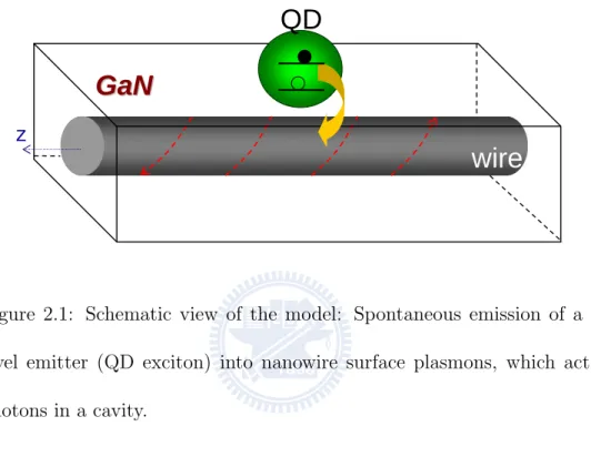
2.1 Schematic view of the model: Spontaneous emission of a two-

level emitter (QD exciton) into nanowire surface plasmons,

which act like photons in a cavity……….7

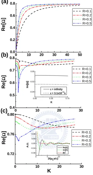
2.2 (a), (b), and (c) represent the dispersion relations of surface

plasmons for the modes n = 0; 1, and 2, respectively. The non-

solid (solid) lines represent the bound (non-bound) modes.

The units for vertical and horizontal lines are Ω=ω/ω

and

K =k

c/ω

, and R=ω

a/c. The inset in (c) represents the

real part, imaginary part, and intensity of the electric field for

n = 1 non-bounded mode as a function of distance away from

the wire surface………...10

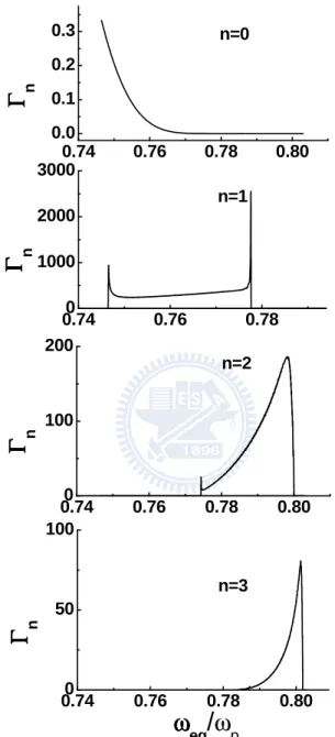
2.3 Spontaneous emission rate (Γ

) into n = 0～3 modes for

R = 0.1. The unit of ¡n is normalized to free space decay rate

γ

………...19

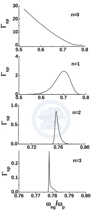
2.4 Spontaneous emission rate (¡n) into n = 0～3 modes for

R = 0.5. The unit of ¡n is normalized to free space decay rate

γ

...20

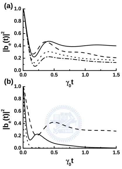
2.5 (a) Non-Markovian decay dynamics of QD excitons forδ=-0.4

γ

(dashed line); 0.4γ

(dotted line); and 0.8γ

(dash-

doted line). Asδ= 0; the solid line represents the result

for the contribution from n = 1 mode. (b) By settingδ= 0,

the dotted, solid, and dashed lines represent the results for

dot-wire separation d = 0.2, 0.3, and 0.35, respectively. Here,

one unit of d is ω

a/c = 53.8 nm………...21

3.1 Schematic view of a metal nano-wire coupled with two QDs.

A single surface plasmon injected from the left is coherently

scattered by the dots………....23

3.2 Transmission probabilities |t|

(dashed lines) and reflection

Probabilities |r|

(solid lines) for a single surface plasmon inci-

dent on two QDs, as a function of detuning δ. In plotting the

figures, we have assumed thatγ

=Γ

=0.025Γ

in (a), and

kd = π/4 in (b). The inset in (a) shows the peak positions

of the reflection probabilities as a function of kd. The green

(blue) line represents the result with (without) super-radiant

effect. The inset in (b) is the result of a surface plasmon inci-

dent on a single dot [16]………..27

3.3 (a) Concurrence C of the two-dot qubits as functions of inter-

dot distance and detuning δ. (b) The phase factor θ of the

entangled state e

|e

, g

>+ e

iθ

e

|g

, e

> in the limit ofγ

→0.

Black, red, and blue lines represent the results of Γ

= 0, 0.025,

and 0.125Γ

, respectively……….34

3.4 The density plot of the concurrence……….35

3.5 Schematic diagram of the storage process into metastable en-

tangled states, |s

, g

> ± |g

, s

> ,with classical optical pulses

wire, a dielectric waveguide is introduced to achieve remote

entanglement……….36

4.1 Schematic diagram of the two quantum dots coupled to two

separate wires with finite length………...38

4.2 Population dynamics without dissipations for each diagonal

Element……….54

4.3 Population dynamics with dissipations (Γ

=γ

=γ

=γ

)

for each diagonal element……….55

4.4 Population dynamics with dissipations (Γ

=Γ

=γ

=γ

=γ

)

for kd = π/2 for each diagonal element………...59

4.5 Population dynamics with dissipations (Γ

=Γ

=γ

=γ

=γ

)

for kd =π/4 for each diagonal element………...60

4.6 Population dynamics with dissipations (Γ

=Γ

=γ

=γ

=γ

)

for kd = 2π for each diagonal element………..61

4.7 The concurrence dynamics without dissipations for kd = (a)

(2n+1)π/2 (n = 0, 1, 2…) (b) (4n+1)π/4 (n = 0, 1, 2…) (c) even

multiple of πand (d) odd multiple of π...63

4.8 The concurrence dynamics with dissipations (Γ

=Γ

=γ

=γ

=

2…) (c) even multiple of π and (d) odd multiple ofπ………...64

4.9 The concurrence dynamics for kd = (2n+1)π/2 (n = 0, 1, 2…)

without dissipations for the ratios g1/g2 =(a) 1/2 (b)1/3 (c) 1/5

and (d) 3/5………...66

4.10 The concurrence dynamics for (a) kd=odd multiple of π with

|Ψ(0)> being the triplet state and (b) kd=even multiple of π

with |Ψ(0)> being the singlet state………..69

4.11 The concurrence dynamics without dissipations. The initial

state is in the mixed state for kd = (a) (2n+1)π/2 (n = 0, 1, 2…)

(b) multiple of π(c) (4n+1)π/4 (n = 0, 1, 2…) and (d) (3n+1)π/3

(n = 0, 1, 2…)………...70

5.1 The schematic diagram for a one-dimensional array to simulate

Bose-Hubbard model……….75

Chapter 1

Introduction

Surface plasmons, generated by collective vibrations of the local charge densities on the metallic surface, are propagating electromagnetic waves along the metal-dielectric interface (See Fig. 1.1). In 1957, Ritchie pioneeringly predicted the existence of the collective excitations of conduction electrons in a thin foil by calculating the energy losses of a fast electron passing through the thin foil [2]. In 1959, Powell an Swan experimentally showed the ex-istence of the collective excitations [3], and the quanta of these excitations are first called ”surface plasmons” in 1960 [4]. Since then, surface plasmons have been extensively studied both in theoretical and experimental investi-gations. Recently, the concept of plasmonics, in analogy to photonics, has received great attention since surface plasmons reveal strong analogies to light propagation in conventional dielectric components [5]. For examples, it

Figure 1.1: Schematic diagram of the surface plasmons [1].

is now possible to confine them to subwavelength scales [1] leading to novel approaches for waveguiding below the diffraction limit [6]. The combination of subwavelength confinement, single mode operation [7], and relatively low power propagation loss [8] of surface plasmon polaritons could be used to miniaturize existing photonic circuits [9], or implement plasmon-based com-putational logic in the THZ regime. In addition, high surface plasmon field confinement was also used to demonstrate an all-optical modulator [10].

Plasmon induced modification of the spontaneous emission (SE) is nat-urally an extended issue [11]. Sun et al. recently calculated the Lamb shift of a hydrogen atom due to the surface plasmon polariton [12]. Strong en-hancement of fluorescence due to surface plasmons was also observed [13]. Coherent coupling between individual optical emitters and guided plasmon excitations in conducting nanowires at optical frequencies was also pointed

out [14]. In chapter 2, we will therefore investigate the spontaneous emission (SE) rate of a quantum dot (QD) exciton into the surface plasmons in a metal nanowire. SE of a QD exciton into different modes of surface plasmons is considered separately. The emission rate is found to approach infinity at cer-tain values of QD exciton bandgap, which is similar to the band-edge effect in photonic crystals. This enhancement has been experimentally observed by Akimov et al. [15] with an enhanced Purcell factor (Γpl/Γ0), which is about

2.5 at room temperature.

In 2007, D. E. Chang et al. proposed a novel approach [16] to form a ”optical transistor” through the scattering of surface plasmons propagating on the surface of a metal wire. In a related context, advances in quantum information science (QIS) has promoted an experimental drive for physical realizations of highly entangled states [17]. Some success has been found within quantum-optical and atomic systems [18]. However, due to scalabil-ity requirements, solid-state realizations of such phenomena are the favored choices [19]. Furthermore, while initial success has been found by concen-trating on coupling nearby qubits with local interactions [20], entangling arbitrary remote qubits is now an important goal. Circuit quantum elec-trodynamics (QED), for example, is one of the few promising candidates to couple two distant qubits via a cavity bus [21]. Motivated by these recent developments, we will in chapter 3 propose a scheme that can achieve the

entanglement between two remote QD qubits coupled to the same metal wire. To increase the efficiency of optical transmission, Pyayt et al. [22] pro-posed that the nanowires lay perpendicular to the polymer waveguide with one end inside the polymer. They theoretically predicted and experimen-tally demonstrated the control over the degree of coupling by changing the light polarization. Furthermore, B. Dayan et al. [23] proposed a ”photon turnstile” to demonstrate an efficient mechanism for the regulated transport of photons one by one by using a microscopic optical resonator evanescently coupled to a fiber. From these, we propose to use two small wires evanescently coupled to a dielectric wave guide instead of using a long wire to increase the transmission efficiency of the surface plasmons in chapter 4. This also enables us to minimize the Ohmic losses during propagation.

More recently, surface plasmon is discovered to be a new dimension to store information [24]. And the basic quantum mechanical property for a quantum particle, that is the duality of surface plasmons, has been also ex-amined [25]. Moreover, in stead of using the conventional far-field optical detection, Falk et al. [26] proposed a new all-electrical surface plasmon po-laritons detection techniques based on the near-field coupling between guided plasmons and a nanowire field-effect transistor to detect the plasmon emis-sion from an individual colloidal quantum dot coupled to a surface plasmon polaritons waveguide. In this way, one could not only preserve the better

ef-ficiency and miniaturization of photonic circuits but also have the advantage of electrically near-field detection.

In the last chapter, we will summarize this thesis and propose a future work on the simulation of quantum phase transition [27, 28] by considering one QD coupled to a small nanowire as a site of a one-dimensional array. Bose-Hubbard model can then be simulated if each site is coupled to its nearest neighbors.

Chapter 2

Spontaneous emission of

excitons into surface plasmons

2.1

Dispersion relations of surface plasmons

Consider now a colloidal CdSe/ZnS quantum dot (QD) near a cylindri-cal silver nanowire with radius a. The QD and nanowire are assumed to be separated by a GaN layer [29] as shown in Fig. 2.1. One of the main rea-sons to choose a CdSe/ZnS QD exciton as the two-level emitter is that it is now possible to isolate single colloidal QD and measure its exciton lifetime [30]. The other reason is that its exciton bandgap is around 2eV to 2.5eV , depending on the size and environment of the dot [31]. The plasmon en-ergy ¯hωp of bulk silver is 3.76 eV with the corresponding saturation energy

¯hωp/

√

2 ≈ 2.66eV in the dispersion relation [32]. As we shall see below, vari-ations of the dispersion relvari-ations in energy just match the exciton bandgap of colloidal CdSe/ZnS QDs.

QD

wire

GaN

GaN

Figure 2.1: Schematic view of the model: Spontaneous emission of a two-level emitter (QD exciton) into nanowire surface plasmons, which act like photons in a cavity.

Surface plasmon modes are created due to the nonzero local charge density on the surface of a nanowire. The n-th surface plasmon mode’s components of the electromagnetic field at the surface can be obtained by solving Maxwell’s equations in a cylindrical geometry (ρ and ϕ denote the radial and azimuthal

coordinates, respectively) with the appropriate boundary conditions [33]: Eρ= [ ikz Kξ dψξ n(Kξρ) d(Kξρ) Aξ n− µξωn K2 ξρ ψξ n(Kξρ)Bnξ]φn, Eϕ = −[ nkz K2 ξρ ψξ n(Kξρ)Aξn− iµξω Kξ dψξ n(Kξρ) d(Kξρ) Bξ n]φn, Ez = [ψnξ(Kξρ)Aξn]φn, Hρ = [ n(K2 ξ + kz2) µξωKξ2ρ ψ_nξ(Kξρ)Aξn+ ikz Kξ dψξ n(Kξρ) d(Kξρ) B_nξ]φn, Hϕ = [ i(K2 ξ + k2z) µξωKξ dψξ n(Kξρ) d(Kξρ) Aξ_n− nkz K2 ξρ ψ_nξ(Kξρ)Bnξ]φn, Hz = [ψnξ(Kξρ)Bnξ]φn, (2.1) with K2 ξ = ω2²ξ(ω)/c2− k2z (ξ = I or O), ψI n(KIρ) = Jn(KIρ), ψnO(KOr) = Hn(1)(KOρ), φn= exp(inϕ + ikzz − iωt),

where Jn(KIρ) and Hn(1)(KOρ) are Bessel and Hankel functions, respectively.

I (O) stands for the component inside (outside) the wire. The dielec-tric function is assumed as ²(ω) = ε∞[1 − ω

2

p

ω(ω+i/τ )], where ²∞ = 9.6 (for

Ag) and ²∞ = 5.3 (for GaN). The plasma energy (¯hωp) of bulk silver is

3.76 eV , and τ = 3.1 × 10−14 _{s is the relaxation time due to ohmic metal}

loss [34], which has been taken into account in the following calculations. The magnetic permeabilities µI,O are unity everywhere since we consider

nonmagnetic materials here. Aξ

n and Bnξ are constants to be determined

by normalizing the electromagnetic field to the vacuum fluctuation energy, R

²(|Eρ|2+ |Eϕ|2+ |Ez|2)dr = ¯hω(k), and matching the boundary conditions.

According to the experiment [35], the length of a nanowire is very long com-paring to the size of the QD. Therefore, it’s legitimate to treat the length of the nanowire as effectively infinite. In this case, the dispersion relations of the surface plasmons with a continuum spectrum can be obtained by solving the following transcendental equation numerically [33]:

S(kz, ω) = [ µI KIa J0 n(KIa) Jn(KIa) − µO KOa Hn(1)0(KOa) Hn(1)(KOa) ][(ω/c) 2_ε I(ω) µIKIa J0 n(KIa) Jn(KIa) −(ω/c) 2_ε O(ω) µOKOa Hn(1)0(KOa) Hn(1)(KOa) ] − n2_k2 z[ 1 (KOa)2 − 1 (KIa)2 ]2 = 0. (2.2)

Fig. 2.2(a) shows the dispersion relations of the n = 0 mode for different radii. Here, one unit of the effective radii R (≡ ωpa/c) is roughly equal to

53.8 nm. As can be seen, the behavior of these curves is very similar to the two-dimensional case [17], i.e. Ω(≡ ω/ωp) gradually saturates with increasing

0 10 20 30 0.4 0.5 0.6 0.7 0.8 0 10 20 30 0.72 0.76 0.80 0 10 20 30 40 50 0.0 0.2 0.4 0.6 0.8 0.00 0.35 0.70 -0.04 -0.02 0.00 Im [[[[ ΩΩΩΩ ]]]] K ττττ = infinity ττττ = 3.1x10-14s 0 5 10 -0.08 -0.04 0.00 0.04 0.08 A .U . D((((ωωωω_pa/c)))) Re[E] Im[E] |E|2

K

(c)

(b)

(a)

Figure 2.2: (a), (b), and (c) represent the dispersion relations of surface plasmons for the modes n = 0, 1, and 2, respectively. The non-solid (solid) lines represent the bound (non-bound) modes. The units for vertical and horizontal lines are Ω = ω/ωp and K = kzc/ωp, and R ≡ ωpa/c. The inset

in (c) represents the real part, imaginary part, and intensity of the electric field for n = 1 non-bounded mode as a function of distance away from the wire surface.

independent of the azimuthal angle ϕ. However, the behaviors for the n 6= 0 modes are quite different as shown in Fig. 2.2(b) and (c). The first interesting point is the discontinuities around ω/c ≈ kz. Further analysis shows that

the solutions of ω are ”almost real” [36] as kz > Re[ω]/c. In this case, the

first kind Hankel function of order n, Hn(1)(Kξρ), decays exponentially. This

means the surface plasmons in this regime are confined on the surface (bound modes). For kz < Re[ω]/c, however, the solutions of ω are complex. The

form of Hn(1)(Kξρ) in this case is like a traveling wave (non-bound modes),

for which its lifetime is finite. One might think that the reason for the finite lifetime is totally from the ohmic metal loss. However, as shown in the inset of Fig. 2.2(b), the frequency is still complex (the solid line) even without the metal loss τ . We thus conclude that the finite lifetime in the regime of kz

< Re[ω]/c is actually influenced by both metal and radiation loss.

2.2

Rate enhancement due to band-edge

ef-fect

To calculate the SE rate of a QD or atom within a structured reservoir, one in general considers the contributions from the scattered fields for different surface geometry of surrounding scatters. There are some well-developed

methods to deal with such calculations. For instance, making use of the Green’s tensors, one can calculate the scattered fields and obtain the local density of states for an atomic dipole [37]. Once the surfaces of scatters are metallic, the presence of surface plasmons are expected to dominate the SE rate due to the strong coupling between surface plasmons and QD [14]. A simple explanation why the coupling is so strong is that the density of energy stored in the electric fields of surface-plasmon modes must be equal to half the vacuum fluctuation energy, 1

2

R

²(|Eρ|2+|Eϕ|2+|Ez|2)dr = 1₂¯hω(k). Since

the volume of the wire is very small, the electric field is supposed to be very strong. In our case, we would like to focus on the decay into surface plasmons on the SE rate, since other contributions of the scattering fields are much smaller than that of the surface plasmons.

The general decay rate of a QD or atom coupled to multi-mode electro-magnetic fields can be directly obtained from Fermi’s golden rule [38] within the dipole approximation:

Γsp =

2π ¯h

Z

d~k |~d0· ~E(~k)|2δ(ωeg− ω_~k), (2.3)

where ω_~k and ~k are the frequency and wave vector of the field ~E(~k), respec-tively. ~d0 is the dipole moment of the QD exciton, and ωeg is the exciton

bandgap of the QD. Once the electromagnetic fields are determined, the SE rate, Γsp, of the QD excitons into bound surface plasmons can be obtained

via Eq. (2.3). Since the surface plasmons are confined on the surface [39] of the cylindrical nanowire, the integral of ~k in Eq. (2.3) stands for the summa-tion of the contribusumma-tions from all possible final states, i.e. a two-dimensional integral of kϕ and kz. Because n is the quantum number governing the

ϕ-component of the wavefunction, summing over all n-mode is equivalent to integrate over all kϕ. For convenience, we assume the dipole moment ~d0 is

along the ρ-direction. By transforming the argument of the delta function from ω_~k(= ωn,kz) to kz as δ(ωeg − ω_~k) = X k_zi 1 |d(ωeg−ωn,kz) dkz |kzi δ(kz − kzi),

the SE rate can then be written as Γsp = ∞ X n=0 Γn= 2π ¯h ∞ X n=0 P k_zi|~d0· ~Eρ(kzi)| 2 |d(ωeg−ω_n,kz) dkz |kzi , (2.4)

where Γn is the SE rate into the n-th mode, and kzi stands for the values

of kz that make the argument in the δ function vanish. For the purpose

of discussion, we display the SE rate into the first few modes (Γn, n =

0, 1, 2, 3) as shown in Fig. 2.3 and 2.4 for R = 0.1 and 0.5, respectively. In plotting Fig. 2.3 and 2.4, the distance between the dot and the wire surface is fixed as ` = 10.76 nm. We find that the latter modes (n > 3) contribute much less to the decay rate. For certain ranges of ωeg, the

contributions to the decay rate Γsp mainly come from the first few modes.

n = 1 mode dispersion curve, the decay rate (for R = 0.1 case) is mainly from n = 0 and n = 1 modes as seen from Fig. 2.3. In addition, the novel feature here is that the SE rate approaches infinity at certain values of the exciton bandgap ωeg. Mathematically, one might think that at these values

the corresponding slopes of the dispersion relation are zero [40]. Physically, however, this infinite rate is not reasonable since it’s based on perturbation theory. Therefore, one has to treat the dynamics of the exciton around these values more carefully, i.e. the Markovian SE rate is not enough. One has to consider the non-Markovian behavior around the band-edge, which means the band abruptly appears/disappears across certain values of ωn,kz.

2.3

Non-Markovian dynamics of QD excitons

When a open quantum system interacts with a structured reservoir, there exists non-Markovian memory effect in the form of oscillatory behav-ior of decay dynamics which reflects the exchanges of information back and forth between system and reservoir. Recently, J. Piilo et al developed a non-Markovian Quantum Jumps method [41] which generalized the proved Monte Carlo wave function method for the Markovian system in order to deal with the non-Markovian problems. Here, we will numerically solve the time-dependent Schr¨odinger equation to obtain the time-time-dependent population on

the excited state.

To obtain the non-Markovian dynamics of the exciton, we first write down the Hamiltonian of the system in the interaction picture (with the rotating wave approximation), Hex−sp = X n,kz ¯h∆n,kzba † n,kzban,kz +¯hX n,kz (gn,kzσgeba † n,kz + g ∗ n,kzσegban,kz), (2.5)

where σij = |ii hj|(i, j = e, g) are the atomic operators; ban,kz and ba †

n,kz are

the radiation field (surface plasmon) annihilation and creation operators; ∆n,kz = ωn,kz − ωeg is the detuning of the radiation mode frequency ωn,kz

from the excitonic resonant frequency ωeg, and gn,kz = ~d0 ·

− →

En,kz is the

atomic field coupling.

Assuming there is an exciton in the dot with no plasmon excitation in the wire initially, the wavefunction of the system then has the form

|ψ(t)i = be(t) |e, 0i +

X

n,kz

bn,kz(t) |g, 1n,kzi e

−i∆n,kzt_{. (2.6)}

The state vector |e, 0i describes an exciton in the dot and no plasmons present, whereas |g, 1n,kzi describes the exciton recombination and a

sur-face plasmon emitted into mode kz. With the time-dependent Schr¨odinger

equation, the solution of the coefficient be(t) in z-space is straightforwardly

ebe(z) = [z + ∞ X n=0 Z gn,kzg ∗ n,kz dkz z + i(ωn,kz − ωeg) ]−1_{. (2.7)}

We use the dispersion relations obtained from Eq. (2.2) to numerically cal-culate the integral over the whole spectrums of n and kz in Eq. (2.7).

Con-sequently, be(t) can be obtained by performing a numerical inverse Laplace

Transformation to Eq. (2.7).

The dashed, dotted, and dash-dotted lines in Fig. 2.5(a) represent the decay dynamics of the QD excitons for different detunings: δ = −0.4γ0, 0.4γ0,

and 0.8γ0, respectively. Here, δ = ω0− ωn=1,kz is the detuning from the local

minimum of the n = 1 mode, and γ0 is the decay rate of the QD exciton into

free space. The radius of the wire and the wire-dot separation are R = 0.1 and ` = 0.34, respectively. Apparently, there exists oscillatory behavior in the decay profile, demonstrating that decay dynamics is non-Markovian. If one considers only the contribution from the n = 1 mode and set the detuning δ = 0, the probability amplitude would saturate to a steady limit as shown by the solid line. This quasi-dressed state is an analogy of Rabi-oscillation in cavity quantum electrodynamics, and also appears in the systems of photonic crystals [42]. In the investigations for SE of a two-level atom near the edge of a photonic band gap, the density of states becomes singular, and the dispersion relation near the band edge can be approximated as a parabolic

curve [42]. The oscillatory behavior during the decay can be then obtained by treating the transition from the excited state to the intermediate state as the other decay channel. The oscillatory behavior in the photonic crystal case is a direct consequence of strong interaction between the atom and its own localized radiation. In our case, the coupling between the QD exciton and surface plasmons can be very strong as well, resulting from a similar feature of local extremum in the dispersion curve. So, the oscillations in decay dynamics shown in Fig. 2.5(a) can be understood as the SE near a band-edge.

Another interesting discovery is shown in Fig. 2.5(b) if one sets the detuning δ = 0 and plots the dynamics of the exciton for different dot-wire separations: ` = 0.2 (dotted line), ` = 0.3 (solid line), and ` = 0.35 (dashed line). As can be seen, the oscillatory behavior is diminished when decreasing the dot-wire separation. This is because, as ωeg is chosen to be close to

the local minimum of the dispersion relation of the n = 1 mode, the decay dynamics is mainly dominated by the contributions from n = 0 and n = 1 modes. Since the non-Markovian oscillatory behavior is mainly from the local minimum of n = 1 mode, the contribution from the n = 1 mode can be overwhelmed by that from the n = 0 mode if the dot is put close enough to the wire surface. This leads to a degradation of the oscillatory behavior.

2.4

Conclusion

In this chapter, we have numerically calculated the dispersion relations of nanowire surface plasmons propagating on the surface of a silver nanowire and have shown that SE of QD excitons into surface plasmons can be greatly enhanced at certain values of the exciton bandgap. The enhancement is due to the strong coupling between QDs and the surface plasmons, and also the band-edge effect [28] in dispersion relation. A non-Markovian way has been used to treat the unreasonable infinitely-enhanced SE rate around the band edge. With this treatment, we observe the oscillatory decay dynamics of QD excitons. This band-edge effect can be analogous to the case that when a two-level atom near the edge of photonic band gap: the density of state is singular and the dispersion curves can be approximated as a parabolic curve coinciding with the local minimum point in our dispersion relations for n ≥ 1 modes.

0.740 0.76 0.78 0.80 50 100 0.740 0.76 0.78 1000 2000 3000 0.74 0.76 0.78 0.80 0.0 0.1 0.2 0.3 0.740 0.76 0.78 0.80 100 200

ΓΓΓΓ

ω

ω

ω

ω

/

ω

ΓΓΓΓ

ΓΓΓΓ

ΓΓΓΓ

Figure 2.3: Spontaneous emission rate (Γn) into n = 0 ∼ 3 modes for R = 0.1.

0.76 0.77 0.78 0.79 0.80 0.0 0.1 0.2 0.5 0.6 0.7 0.8 0 2 4 0.5 0.6 0.7 0.8 0 10 20 30 0.72 0.76 0.80 0.0 0.5 1.0

ΓΓΓΓ

ω

ω

ω

ω

/ω

ω

ω

ω

ΓΓΓΓ

ΓΓΓΓ

ΓΓΓΓ

Figure 2.4: Spontaneous emission rate (Γn) into n = 0 ∼ 3 modes for R = 0.5.

0.0 0.5 1.0 1.5 0.0 0.2 0.4 0.6 0.8 1.0 0.0 0.5 1.0 1.5 0.0 0.2 0.4 0.6 0.8 1.0

|b

(t

)|

γγγγ

t

(b)

|b

(t

)|

γγγγ

t

(a)

Figure 2.5: (a) Non-Markovian decay dynamics of QD excitons for δ = −0.4γ0 (dashed line), 0.4γ0 (dotted line), and 0.8γ0 (dash-doted line). As

δ = 0, the solid line represents the result for the contribution from n = 1 mode. (b) By setting δ = 0, the dotted, solid, and dashed lines represent the results for dot-wire separation d = 0.2, 0.3, and 0.35, respectively. Here, one unit of d is ωpa/c = 53.8 nm.

Chapter 3

Coherent single surface

plasmon transport

3.1

Scattering of surface plasmons

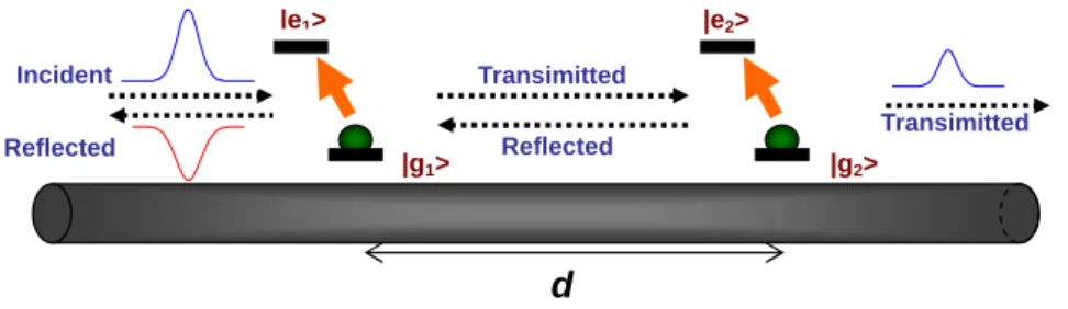
We propose in this chapter a novel scheme that can entangle two remote QD qubits coupled to a metal nanowire. The idea is inspired by recent experiments showing single surface plasmons in metallic nanowires coupled to QDs [15]. We will use a real-space Hamiltonian to treat the coherent surface-plasmon transport in the wire coupled to two dots. It will be found maximally entangled states can be created if the separation between the two dots is equal to multiple half-wavelength of the optical plasmon. Furthermore, we will show the entangled state can also be stored in the metastable states,

d Transimitted Reflected Incident Reflected

Figure 3.1: Schematic view of a metal nano-wire coupled with two QDs. A single surface plasmon injected from the left is coherently scattered by the dots.

which are decoupled from the surface plasmons, by applying classical laser pulses to each QD separately. The storage efficiency of the entangled states is equal to 1 − 1/P , where P is the Purcell factor of the QD excitons.

When a semiconductor QD is put close to a metal nanowire, strong cou-pling between the QD exciton and surface plasmons can occur [14], as in traditional cavity QED. In the following, we consider two QDs, separated by a distance of d, near a cylindrical metal nanowire with radius a as shown in Fig. 3.1. The Hamiltonian of the two-level QDs (with energy spacing ¯hωeg)

H = X j=1,2 ¯h[ωeg− i( γ0+ Γ0 2 )]σej,ej −i¯hsin(k0d) 2k0d γ0(σe1,e2 + σe2,e1) −¯hg Z dk [(σe1,g1 + σe2,g2e ikd_)a k+ h.c.] + Z dk ¯hvg|k|a†kak, (3.1)

where σej,ej(σej,gj)= |ejihej|(|ejihgj|) represents the diagonal (off-diagonal)

element of the j-th QD operator, and a†_k is the creation operator of the surface plasmon. Here, γ0 and Γ0 denote the decay rates into free space and

other non-radiative channels, respectively. vg is the velocity of the surface

plasmon, k0 = ωeg/vg, and g is the coupling constant between the excitons

and surface plasmons. The third term in the first line of Eq. (3.1) represents the effect of collective decay (super-radiance) [44]. Transforming Eq. (3.1) into real space, one obtains

H = ¯h Z dx{−ivgc†R(x) ∂ ∂xcR(x) + ivgc † L(x) ∂ ∂xcL(x) +¯hg X j=1,2 δ(x − (j − 1)d)[c†_R(x)σgj,ej+ cR(x)σej,gj +c†_L(x)σgj,ej + cL(x)σej,gj]} +X j=1,2 [Ee− i¯h( γ0 + Γ0 2 )]σej,ej −i¯hsin(k0d) 2k0d γ0(σe1,e2+ σe2,e1) + Egσgj,gj, (3.2)

where Ee − Eg = ¯hωeg and c†R(x) [c†L(x)] is a bosonic operator creating a

right-going (left-going) photon at x. Assuming that a photon is coming from the left with energy Ek = vgk. The stationary state of the system is written

as |Eki = Z dx[φ†_k,R(x)c†_R(x) + φ_k,L† (x)c†_L(x)]|g1, g2, 0i + X j=1,2 ekjσej,gj|g1, g2, 0i, (3.3)

where |g1, g2, 0i means that both QD-1 and -2 are in the ground state with

zero photon and ekj is the probability amplitude of the j-th QD in the excited

state. For a photon incident from the left, φ†_k,R(x) and φ†_k,L(x) takes the form        φ†_k,R(x) ≡ exp(ikx)[θ(−x) + a θ(x)θ(d − x) + t θ(x − d)], φ†_k,L(x) ≡ exp(−ikx)[r θ(−x) + b θ(x)θ(d − x)], (3.4)

where t and r are the transmission and reflection amplitudes, respectively. a exp(ikx)θ(x)θ(d − x) and b exp(−ikx)θ(x)θ(d − x) represent the wave-function of the photon between 0 and d. From the eigenvalue equation H|Eki = Ek|Eki, we obtain the following relations for the coefficients

                      

g(2aeikd_{+ 2be}−ikd_{) −} i

2 sin(k0d) kd γ0ek1 = (Ek/¯h − ωeg)ek2, g(1 + a + r + b) − i 2 sin(k0d) k0d γ0ek2 = (Ek/¯h − ωeg)ek1, gek1 = ivg(a − 1), a = r − b + 1, gek2 = ivg(t − a)e

ikd_{, and t = a + be}−2ikd_.

The transmission and reflection amplitudes can then be determined alge-braically.

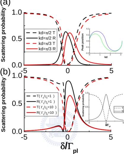
Fig. 3.2(a) numerically displays the transmission coefficients |t|2 (dashed lines) and reflection coefficients |r|2 (solid lines) for different inter-dot dis-tance. It is evident that the peak positions of the reflection coefficients deviate from the center (δ = 0). The inset in Fig. 3.2(a) shows the peak positions as a function of kd. The green (blue) line represents the result with (without) super-radiant effect. As can be seen, not only the interference from the inter-dot separation, but also the super-radiance affects the positions of the peaks. Fig. 3.2(b) shows that the amplitude of reflection coefficients is suppressed when increasing metal loss Γ0. Another interesting point is that

the reflection coefficients have minimum points in the regime of δ < 0. In the limit of large d, the super-radiant effect can be neglected. By setting Γ0 _{= γ}

0+ Γ0, the positions of the minimum points, δmin, can be deduced from

Eq. (3.5) and satisfy the following relation: − tan2_{(kd) = −4(}δmin

Γpl

)2 _{− (}Γ0

Γpl

)2_{. (3.6)}

If there is no reflection (r = 0), one can say that Eq. (3.6) is the resonant tunneling condition for a photon travelling through two QDs, as an electron tunnel through a barrier.

-5

0

5

0.0

0.5

1.0

-5

0

5

0.0

0.5

1.0

δδδδ

/

ΓΓΓΓ

pl

(b)

(a)

Figure 3.2: Transmission probabilities |t|2 (dashed lines) and reflection prob-abilities |r|2(solid lines) for a single surface plasmon incident on two QDs, as a function of detuning δ. In plotting the figures, we have assumed that γ0 = Γ0 = 0.025Γpl in (a), and kd = π/4 in (b). The inset in (a) shows

the peak positions of the reflection probabilities as a function of kd. The green (blue) line represents the result with (without) super-radiant effect. The inset in (b) is the result of a surface plasmon incident on a single dot [16].

3.2

Entanglement creation and storage

Eq. (3.3) and Eq. (3.5) also tell us that if there is no transmission or reflection photon detected at the two ends of the wire, the wavefunction col-lapses into the state: P_j=1,2ekjσej,gj|g1, g2, 0i. This means that it is possible

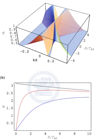
to create entanglement between the two dots. Two special cases are that if kd = 2nπ or (2n + 1)π with n being an integer, the amplitude ek1 is equal to

ek2 or −ek2, respectively. In this case, the two-dot qubits become triplet or

singlet entangled if no photon is detected. Fig. 3.3(a) shows the concurrence C of the two-dot qubits as functions of inter-dot distance and detuning δ. In addition to the special cases mentioned above, there is another oblique line satisfying the condition of maximum entanglement (C = 1). In the limit of large d, we find that the equation of this line is give by

δ = −(Γpl+ Γ0) tan(kd). (3.7)

The physical meaning is that even the energy of the incident photon is not res-onant with the qubit energy ¯hωeg, it is still possible to achieve the maximum

entangled states, only if the two dots are put at the right positions. The price to pay is that the entangled state now becomes ek1|e1, g2i+ eiθ·ek2|g1, e2i, i.e.

there is an extra phase θ between |e1, g2i and |g1, e2i. Fig. 3.3(b) shows the

black, red, and blue lines represent the results of Γ0 = 0, 0.025, and 0.125Γpl,

respectively. As can be seen, once the metal loss, Γ0, appears, the phase

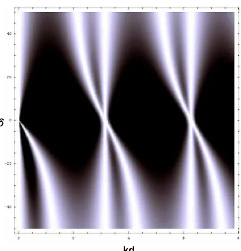
in-stantaneously changes from π(black line) to 0(red and blue lines) at the point δ = 0. In Fig. 3.4, we show the density plot of the Concurrence versus kd and δ. The two different cases of maximal entanglement can be clearly seen. One might argue that the created entangled states are irrelevant since the QDs are still coupled to the surface plasmons. The entanglement would even-tually disappear due to radiative or non-radiative loss. To overcome this, one can consider multilevel emitters, such as the three-level configuration shown in Fig. 3.5. Metastable states, |s1i and |s2i, are decoupled from the

sur-face plasmons, but are resonantly coupled to |e1i and |e2i, respectively, via

a classical optical control field with Rabi frequencies Ω1(t) and Ω2(t).

Instead of transforming Eq. (3.1) into real space, the Hamiltonian is now represented under the bases of singlet, |Si = _√1

2(|e1, g2i − |g1, e2i), and

triplet, |T i = _√1 2(|e1, g2i + |g1, e2i, states: H = ¯h(ωeg− i Γ0 2)(|T i hT | + |Si hS|) −¯hg Z dk {[√1 2(1 + e ikd_{) |T i hg} 1, g2| ak +√1 2(1 − e ikd_{) |Si hg} 1, g2| ak] + h.c.} + Z dk ¯hvg|k|a†kak, (3.8)

where Γ0 _{= γ}

0+ Γ0 again is from the approximation that super-radiant effect

can be neglected in the limit of large d. We now consider the general time-dependent wave function

|ψi = Z dk[cR,k(t) ∧ a†_R,k+ cL,−k(t) ∧ a†_L,−k] |g1, g2; vaci +cT(t) |T ; vaci + cS(t) |S; vaci (3.9) +cMT(t) |MT; vaci + cMS(t) |MS; vaci ,

where |MSi[= √1₂(|s1, g2i − |g1, s2i)] and |MTi[= √1₂(|s1, g2i + |g1, s2i)]

de-note the singlet and triplet metastable states, respectively. From H |ψi = −¯h

i∂t∂ |ψi, the state amplitudes evolve according to

· cR,k(L,−k)(t) = −iδkcR,k(L,−k)(t) + ig √ 2(1 + e −ikd_)c T(t) +√ig 2(1 − e −ikd_)c S(t), (3.10)

where δk = vgk − ωeg. If Ω1(t) = Ω2(t) and kd = 2nπ, where n is an integer,

Eq. (3.10) can be substituted into the equation of motion for cT(t)

· cT(t) = − Γ0 2cT(t) + iΩ1(t)cMT(t) +ig Z dk[cR,k(t) + cL,−k(t)], (3.11)

which yields integral-differential equation involving cT(t). Imposing a

at the end, such that cR,k(L,−k)(∞) = 0, one can obtain an implicit

expres-sion for the required pulse shape Ω1(t) and the following equation relating

the population in the state |MTi

d dt|cMT(t)| 2 _{= −v}2 g/(2πg2)( d dt|ET(t)| 2₋ Γpl− Γ0 2 |ET(t)| 2_{), (3.12)} where ET(t) = − √

2πigcT(t)/vg. With the normalizing condition,

R_∞

−∞dt |ET(t)|

2 ₌

1/(2vg), and assuming that the incoming field vanishes at t = ±∞ [ET(±∞) =

0] [16], Eq. (3.12) can be integrated to yield |cMT(±∞)|

2 _{= 1 − 1/P ,}

where P ≡ Γpl/Γ0 is the effective Purcell factor. Similarly, it can be

eas-ily shown that the storage efficiency into |MSi state is also equal to 1 − 1/P

if Ω1(t) = −Ω2(t) and kd = (2n + 1)π. Note that the metal and radiative

losses on the qubits are taken into account in the above derivation. There-fore, the entangled states can be stored with a high efficiency only if the Purcell factor is high enough. Furthermore, the two qubits can be separated in a remote sense, such that one can address a lone qubit without affecting another.

3.3

Remark on experimental realization

Once the entangled state is prepared, how can one verify it? One possible procedure is to inject plasmons from one end and measuring the output

sig-nals. For example, if the entangled state |s1, g2i + |g1, s2i is created, we then

inject a plasmon from the left-side. As the plasmon arrives dot-1, pumping it with a energy-selected laser pulse, which only excites dot-1 from ”g1” state to

”e1” state (but can not excite it from ”s1” to ”e1”). The state now becomes

|s1, g2i + |e1, s2i. Put two detectors at both ends of the wire. If we get a

sig-nal from the right-end, we know that the wave-function collapses into |e1, s2i

(note that the injected plasmon connects the states ”e” and ”g”). Driving the state goes back to |g1, s2i with an appropriate pulse. Then, injecting a

surface plasmon again, but with a pulse on dot-2. This time the surface plas-mon will be scattered by |g1, s2i since dot-1 is in ”g” state and one observes

a signal at the left-end. However, if one observes a signal from the left-end initially, we know that the state collapses into |s1, g2i. When the last pulse

is shined on dot-2, the state becomes |s1, e2i. This time the second plasmon

will pass through the two dots without reflection, and one observes a signal at the right-end. As for the non-entangled state, for example: |s1, s2i/|g1, g2i

state, the above procedure gives two transmitted/reflected photons at at the right/left end.

3.4

Conclusion

In summary, we have examined the scattering properties of the surface plasmons in a metal nanowire coupled with two QDs. Not only the metal loss, but also the super-radiant effect is found to influence the reflection prop-erties. A scheme to create remote entangled state is proposed in the presence of metal and radiative losses. We discover that there are two different cases that the maximal entanglement can be achieved. One is when kd is multiple of π, and the other one is when kd and δ satisfy the condition Eq. (3.7). Furthermore, the proposal can also be applied to other physical system. For example, one can easily extend this to the transmission lines (photons) cou-pled with Cooper pair boxes (qubits). The Hamiltonian is identical to that in Eq. (3.1) [45]. We therefore believe that it could be tested with current technologies.

HaL -0.2 0 0.2 kd -4 -2 0 2 4 δêΓpl 0.5 0.6 0.7 0.8 0.9 1 C -0.2 0 0.2 kd HbL 0 2 4 6 8 10 δêΓpl 0.5 1 1.5 2 2.5 3 θ

Figure 3.3: (a) Concurrence C of the two-dot qubits as functions of inter-dot distance and detuning δ. (b) The phase factor θ of the entangled state ek1|e1, g2i + eiθ · ek2|g1, e2i in the limit of γ0 → 0. Black, red, and blue lines

kd

δ

δ

δ

δ

ٛٛٛٛ |g1 > ٛٛٛٛ|s1 >ٛٛٛٛ d Ω Ω Ω Ω1(t) ΩΩΩΩ2(t) ٛٛٛٛ|e1 >ٛٛٛٛ ٛٛٛٛ|e2 >ٛٛٛٛ ٛٛٛٛ |g2 > ٛٛٛٛ|s2 >ٛٛٛٛ

Figure 3.5: Schematic diagram of the storage process into metastable entan-gled states, |s1, g2i ± |g1, s2i , with classical optical pulses Ω1(t) and Ω2(t).

To avoid the possible losses in metal nano-wire, a dielectric waveguide is introduced to achieve remote entanglement.

Chapter 4

Entanglement dynamics

The surface plasmons inevitably experience losses as they propagate along the nanowire. It could limit the feasibility in creating remote entanglement. To avoid this, instead of using a infinite long silver nanowire, we consider in this chapter two separate wires with finite length (in the order of 10 nm) evanescently coupled to a phase-matched dielectric waveguide [23]. We also assume the two QDs are coupled to these two wires as shown in Fig. 4.1. In this case, one can have both the advantages of strong coupling from the surface plasmons and long-distance transport by the dielectric waveguide.

By using density matrix treatment and Lindblad form master equations, we will investigate the dynamics of the QD excitons and the corresponding entanglement in this chapter.

d

dielectric waveguide

ٛٛٛٛ|g1 > |g2 >

ٛٛٛٛ |e1 > ٛٛٛٛ|e2 >

Figure 4.1: Schematic diagram of the two quantum dots coupled to two separate wires with finite length.

4.1

Open quantum system

Let us assume a system S in a superposition of its two basis states, and a second system S’ is in a initial state |φ0i. If there is no interactions (i.e.

no correlations) between S and S’, the composite state can be written as |Ψi = (α |Ai + β |Bi) ⊗ |φ0i, where|α|2 + |β|2 = 1. If we represent this

separable state as a density matrix ρSS0 = |Ψi hΨ|, and trace out the second

system S’ (i.e. ρS = T rS0ρ_SS0 = hφ₀|Ψi hΨ| φ₀i), we obtain a pure state

reduced density matrix of system S

σS =     |α|2 αβ∗ α∗_{β |β|}2     .

But if the system S interacts with the second system S’, we say that now the system S is ”open”, which causes the evolution of S’. Therefore,

the state of S’ would no longer be in |φ0i and the composite state is not

separable anymore. We can thus write the interacting composite state as |Ψi = α |Ai |φ1i + β |Bi |φ2i. After tracing out the second system S’, we

again obtain the reduced density matrix σS,

ρS =     |α|2 αβ∗_hφ 2|φ1i α∗_{β hφ} 1|φ2i |β|2     .

The off-diagonal elements (coherence) is smaller than those in non-interacting case since hφ2|φ1i < hφ0|φ0i = 1 . This means that the coherence is decreased

due to the interactions between systems S and S’, and the state goes from pure to mixed. In other words, some information of the total system is stored in the entanglement between S and S’ resulting from the coupling [46].

In the third section of this chapter, we will treat the surface plasmon modes as the second system S’, and the two QDs as the system S. From previous discussions, one realizes that the coherence will be decreased due to the QD-plasmon interactions, and the reduced density matrix will become mixed. To investigate the evolution of the reduced density matrix, in the next section, we will introduce the Lindblad form master equation approach, which is widely used to study time-dependent behaviors.

4.2

Lindblad form master equation

Surface plasmons, propagating electromagnetic waves on the surface of metal nanowires in our model, must be damped due to Ohmic losses or the leakages during transmission (see Fig. 4.1). For two QDs, if they are initially in the ground state, each of them is possible to be excited by the surface plas-mons. But meanwhile, they are coupled to the vacuum as well. Therefore, besides decaying into surface plasmons modes, they may also decay into the free space. Since now we consider small nanowires with finite length, the Ohmic losses could be minimized. And, from our previous discussions in chapter 2, the pheonmenon of large Purcell factors due to the strong cou-pling between dots and surface plasmons should still hold. Thus, we can take these two decay channels : field dampings and spontaneous emissions into free space, as dissipations in our model. Instead of using the quantum jump effective Hamiltonian, we introduce in this section the Lindblad form master equation approach [47], in which the two dissipations are both included.

We start out with a general Hamiltonian, H = HS + HR + HSR, where

HS and HR are Hamiltonian for S and R respectively, HSR is the interaction

between system S and reservoir R. The density matrix corresponding to the total system S ⊕ R reads ρSR = ρS ⊗ ρR, while the reduced density matrix of

The Schr¨odinger equation of ρSR is

˙ρSR =

1

i¯h[H, ρSR], (4.1)

we can transform this Schr¨odinger equation into the interaction picture and get

˙˜ρSR= 1

i¯h[ ˜HSR(t), ˜ρSR], (4.2)

with ˜ρSR= ei/¯h(HS+HR)tρSR(t)e−i/¯h(HS+HR)t, and ˜HSR(t) = ei/¯h(HS+HR)tHSR(t)e−i/¯h(HS+HR)t.

Setting the starting point of interaction is t = 0 and integrating Eq. (4.2), we directly obtain ˜ ρSR(t) = ˜ρSR(0) + 1 i¯h Z _t 0 dt0_{[ ˜H} SR(t0), ˜ρSR(t0)]. (4.3)

Substituting this back to Eq. (4.2) for ˜ρSR(t) inside the commutator gives

˙˜ρSR= 1 i¯h[ ˜HSR(t), ˜ρSR(0)] − 1 ¯h2 Z _t 0 dt0_{[ ˜H} SR(t), [ ˜HSR(t0), ˜ρSR(t0)]], (4.4)

where, ˜ρSR(0) = ρSR(0) = ρS(0)ρR(0). Because the system S is what we are

interested in, after tracing out R, Eq. (4.4) becomes ˙˜ρS = 1 i¯hT rR{[ ˜HSR(t), ˜ρSR(0)]} − 1 ¯h2 Z _t 0 dt0_{T r} R{[ ˜HSR(t), [ ˜HSR(t0), ˜ρSR(t0)]]}. (4.5) Since one could always write ˜HSR as a sum of products of operators si of

system S and operators Ri of reservoir R,

˜ HSR(t) = ¯h X i ˜ si(t) ˜Ri(t), (4.6)

we assume that the mean value of the observable ˜Ri in state ρR is zero ( i.e.

T r[ρRR˜i] = 0 ). We can then eliminate the leading term _i¯1_hT rR{[ ˜HSR(t), ˜ρSR(0)]}

with the cyclic property of trace T r[ABC] = T r[BCA] = T r[CAB]. Finally, we have ˙˜ρS = − 1 ¯h2 Z _t 0 dt0T rR{[ ˜HSR(t), [ ˜HSR(t0), ˜ρSR(t0)]]}. (4.7)

If the interaction between the system and reservoir is very weak and the reservoir is relatively large, one can expect the reservoir is virtually unaffected (stay in initial state) during the interaction. Thus, the density matrix of the total system can be expanded as

˜

ρSR(t) = ˜ρS(t)˜ρR(0) + O(HSR), (4.8)

The Born approximation can be made here to neglect the higher order terms in Eq. (4.7) and give

˙˜ρS = − 1 ¯h2 Z _t 0 dt0_{T r} R{[ ˜HSR(t), [ ˜HSR(t0), ˜ρS(t0)˜ρR(0)]]}. (4.9)

We can now substitute Eq. (4.6) into Eq. (4.9) and obtain ˙˜ρS = − X i,j Z _t 0 dt0_{[˜s i(t)˜sj(t0)˜ρS(t0) − ˜sj(t0)˜ρS(t0)˜si(t)]h ˜Ri(t) ˜Rj(t0)iR + [˜ρS(t0)˜sj(t0)˜si(t) − ˜si(t)˜ρS(t0)˜sj(t0)]h ˜Rj(t0) ˜Ri(t)iR}, (4.10) where, h ˜Ri(t) ˜Rj(t0)iR = T rR[˜ρR(0) ˜Ri(t) ˜Rj(t0)] h ˜Rj(t0) ˜Ri(t)iR = T rR[˜ρR(0) ˜Rj(t0) ˜Ri(t)]. (4.11)

Now, we can use this master equation, i.e. Eq. (4.10), to discuss the two dissipations taking place in our model separately. First, we focus on the field damping dissipation and ignore two QDs for present discussion. Considering the surface plasmon modes as a system, and the modes which damp the surface plasmon fields as a reservoir. The Hamiltonian can be written as

HS = X k ¯hωka†_kak, HR = X j ¯hω0_jb†_jbj, HSR = X k,j ¯h(κ∗ j,kakb†j + κj,ka†kbj), (4.12)

where ωk is the energy of the surface plasmons, a†_k(ak) denotes the creation

(annihilation) operators for each k mode; b†_j and bj represent the modes of

reservoir with frequencies ω0

j; κj,k denotes the coupling constant between the

surface plasmons and reservoir. In our model, these j modes play the role of transmission losses from Ohmic losses and the leakages between dielectric waveguide and nanowires. From Eqs. (4.6) and (4.12), we can specify ˜si and

˜ Ri respectively as ˜ s1 = X k ake−iωkt, ˜ s2 = X k a†_keiωkt_, ˜ R1 = ˜R†= X j κ∗ j,kb†jeiω 0 jt, ˜ R2 = ˜R = X j κj,kbje−iω 0 jt. (4.13)

Substitute Eq. (4.13) into Eq. (4.10), we obtain ˙˜ρS = − X k Z _t 0 dt0_{[a kakρ˜S(t0) − akρ˜S(t0)ak]e−iωk(t+t 0₎ h ˜R†_{(t) ˜R}†_(t0_)i R+ h.c. + [a†_ka†_kρ˜S(t0) − ak†ρ˜S(t0)a†k]eiωk(t+t 0₎ h ˜R(t) ˜R(t0_)i R+ h.c. + [aka†kρ˜S(t0) − ak†ρ˜S(t0)ak]e−iωk(t−t 0₎ h ˜R†_{(t) ˜R(t}0_)i R+ h.c. + [a_k†akρ˜S(t0) − akρ˜S(t0)a†k]eiωk(t−t 0₎ h ˜R(t) ˜R†_(t0_)i R+ h.c.}, (4.14)

where we take the reservoir S to be a thermal equilibrium mixture of states, ˜

ρR =

Q

je−¯hω 0

jb†jbj/kBT_{(1 − e}−¯hω0j/kBT_{). Then, we can easily have}

h ˜R†(t) ˜R†(t0)iR = 0 h ˜R(t) ˜R(t0)iR = 0 h ˜R†_{(t) ˜R(t}0_)i R = X j |κj,k|2eiω 0 j(t−t0)n(ω0 j, T ), h ˜R(t) ˜R†_(t0_)i R = X j |κj,k|2e−iω 0 j(t−t0)[n(ω0 j, T ) + 1], (4.15) with n(ω0 j, T ) = T rR(˜ρRb†jbj) = e −¯_hω0j/kBT

1−e−¯hω0j/kBT, is the mean photo number for a

oscillator with frequency ωj at temperature T. Here, kB is the Boltzmann’s

constant. We can make a change of variable τ ≡ t − t0_{, Eq. (4.14) then}

becomes ˙˜ρS = − X k Z _t 0 dτ {[aka†_kρ˜S(t − τ ) − a†_kρ˜S(t − τ )ak]e−iωk(τ )h ˜R†(t) ˜R(t − τ )iR+ h.c. + [a†_kakρ˜S(t − τ ) − akρ˜S(t − τ )a†k]eiωk(τ )h ˜R(t) ˜R†(t − τ )iR+ h.c.}. (4.16)

For a large reservoir containing infinite modes, we can also change the sum-mation in Eq. (4.15) to an integration by introducing the density of state