腦部結構差異量化分析之區塊多變量型態法

國

立

交

通

大

學

生醫工程研究所

碩

士

論

文

腦部結構差異量化分析之

區塊多變量型態法

Parcellation-based Multivariate Morphometry for

Characterizing Differences of Brain Structures

研 究 生：林育宏

指導教授：陳永昇 教授

腦部結構差異量化分析之區塊多變量型態法

Parcellation-based Multivariate Morphometry for Characterizing

Differences of Brain Structures

研 究 生：林育宏 Student：Yu-Hung Lin

指導教授：陳永昇 Advisor：Yong-Sheng Chen

國 立 交 通 大 學

生 醫 工 程 研 究 所

碩 士 論 文

A Thesis

Submitted to Institute of Biomedical Engineering College of Computer Science

National Chiao Tung University in partial Fulfillment of the Requirements

for the Degree of Master

in

Computer Science

June 2009

Hsinchu, Taiwan, Republic of China

摘 要

磁振造影已經成為主要的醫療成像技術，用於了解腦部或是身體上的結構以 及功能，它不僅廣泛應用於臨床診斷，而且在神經影像學研究。近年來，以體素 為基礎的形態計量學 (voxel-based morphometry, VBM) 最常被使用於研究分析 群體間大腦結構的差異性，以比較每一個體素的方式來找出其差異性。 VBM 以 統計的方式量化分析群組間的差異性，這個以體素為基礎的分析方法有能力上的 限制，導致它無法偵測群組織間細微的變化。根據我們的經驗指出，同時地將所 有的體素一起做分析會使區域間不相關的體素相互影響，這樣的分析方法是不恰 當的。 本研究中我們提出了一個新的腦部結構分析方法，以區域為單位的多變量形 態計量學方法，可用於偵測群組間腦部結構的差異性。與體素為基礎的分析方法 相比較之下，我們提出的方法是同時考慮一個區域下所有的體素以多變量的方式 來分析群組間腦部結構的差異性，而最重要的是我們將腦部結構區分成許多個小 區域，藉此達到在相同區域下的所有體素有相同的關聯性。多變量的方法是採用 線性鑑別度分析 (linear discriminant analysis, LDA) 是用來找出對於群組 間結構差異性最具鑑別力的投影軸。位於該投影軸上的每一元素代表相對映體素 具有的差異性鑑別能力。此鑑別能力可以視為用來評估影像群組間每一體素結構 差異之程度等級 (significance level)。

我們的實驗方法包含了兩個部分，第一個部分是透過模擬一個區域的萎縮， 用來驗證以區域為單位的多變量型態計量法的效能，另一個是應用在重性抑鬱障 礙 (Major depressive disorder) 以及雙極性情感疾病 (Bipolar disorder) 的腦部結構分析。透過比較可以了解，以區域為單位的多變量型態計量法確實可 偵測到群組間較細微的搞部結構差異。而此方法也比以體素為基礎的形態計量法 更明顯地找出和病理上相關的腦部結構差異。 總結，我們提出了一個新的腦部結構分析方法，這個方法是以區域為單位的 分析群組間的差異，而且所採用的多變量方法不會有資訊上的遺失，在分析時能 更用更多的資訊更有效地分析腦部結構細微的差異性。 i

誌謝 感謝陳永昇老師和陳麗芬老師兩年的辛苦指導，老師在碩一時總是鼓勵我們 認真的修課，希望我們不要因為研究進度而不認真修課，讓我們在碩一時學到了 很多，在碩二的時候便要求我們認真的做研究，讓我們學習做研究的過程。還有 每到寒暑假以及年終實驗室也會舉辦許許多多有趣的活動，不管是出遊還是尾牙 大家都很開心的玩在一起，研究所這兩年有老師的指導我很珍惜。 也要感謝我身邊的朋友和實驗室同學，不論是一起打球、跑步、吃好料，唱 歌還是一起上課、玩遊戲，有你們的陪伴，讓我度過了快樂的兩年。 最後要感謝我的家人還有我的女朋友，因為你們的照顧以及不時的給我信心 還有給了我許多寫作上的建議，以完成我的碩士論文順利畢業，我很感激，謝謝 你們。 ， iii

Parcellation-based Multivariate Morphometry

for Characterizing Differences of Brain

Structures

A thesis presented by

Yu-Hung Lin

to

Institute of Biomedical Engineering

College of Computer Science

in partial fulfillment of the requirements for the degree of

Master

in the subject of

Computer Science

National Chiao Tung University Hsinchu, Taiwan

2009

Copyright c 2009 by

Yu-Hung Lin

Abstract

Magnetic resonance imaging (MRI) has become primarily a medical imaging technique to visualize the structure and function of the body or brain. It is widely used not only in clinical diagnosis but also in neuroimaging research. In recent years, voxel-based mor-phometry (VBM) is one of the most popular technique for the analysis of structural brain discrepancy between different subject groups, in a voxel-wise manner. VBM analysis de-tects group differences by voxel-wise statistics comparisons which have limited power to identify subtle differences between two populations. And according to our experience, we figure out that when dealing with all features simultaneously, features in different regions of whole brain may be unrelated with each other it is incorrect that we take all features into consideration at one time.

In this work, we propose a parcellation-based multivariate morphometry method which can be used to detect the anatomical discrepancy in brain between two groups. Compared to the voxel-wise manner in VBM, the proposed method detects brain discrepancy in a multivariate manner by simultaneously taking all voxels within an area (or a region) in consideration. The most important idea is that we divide brain into several parts when analyzing such that all features in the same region may be correlated with each other. Linear discriminant analysis (LDA) is used to determine the most discriminant projection vector, also called a discriminant map separating two populations. Each parameter of the most discriminant vector represents the discrimination level of each voxel. That is, based on the discriminant map, each parameter stands for a significant level with each voxel.

To demonstrate the performance of the parcellation-based multivariate method, we car-ried out experiments by using the simulation data set and on a real medical data composed of MRI of subjects with major depressive disorder (MDD) and bipolar disorder (BD). The results with simulation data analysis have shown that the parcellation-based multivariate method has a better performance than VBM from the area under the ROC curve by compar-ing to VBM method. The results with real data analysis have also shown that our proposed method reveals several important findings.

In conclusion, we have proposed a parcellation-based multivariate method for charac-terizing group differences. And all voxels within the same region are simultaneously taken

based multivariate morphometry analysis has a good performance on subtle and widely-distributed structural difference and it is more flexible within analysis.

Contents

List of Figures xi

List of Tables xiii

1 Introduction 1

1.1 Background . . . 2

1.1.1 Brain Structures . . . 2

1.1.2 Magnetic Resonance Imaging (MRI) . . . 6

1.2 Morphometrics . . . 8 1.3 Thesis Motivation . . . 10 1.4 Related Works . . . 11 1.5 Thesis Organization . . . 13 2 Voxel-based Morphometry 15 2.1 Introduction . . . 16 2.2 Optimized VBM Protocol . . . 20 2.3 Implementation of VBM . . . 24 2.4 Drawbacks of VBM . . . 29

3 Parcellation-Based Multivariate Morphometry 31 3.1 Introduction . . . 32

3.2 Framework of Parcellation-Based Multivariate Morphometry . . . 33

3.3 Multivariate Analysis using a Modified LDA-Based Method . . . 37

3.3.1 Conventional Linear Discriminant Analysis and Its Potential Problem 37 3.3.2 Discriminative Common Vector Method . . . 40

3.3.3 The Problem of Combining The Unit Projection Vector . . . 43

4 Experiment Results 45 4.1 Simulation Analysis . . . 46

4.1.1 Simulation Data Generation . . . 46

4.1.2 Accuracy Evaluation . . . 47

4.1.3 Comparisons of Proposed Method and VBM . . . 51 ix

4.2.2 MRI acquisition . . . 54

4.2.3 Results and Comparisons of PBM and VBM . . . 55

5 Discussion 83 5.1 Using the Parcellation-Based Approach . . . 84

5.2 Different Size of Each Region . . . 84

5.3 Limitations of the Atrophy Simulation Package . . . 85

5.4 Why the Smoothing is Eliminated . . . 86

6 Conclusions 89

Bibliography 93

List of Figures

1.1 Brain structures . . . 3

1.2 MR image . . . 4

1.3 Brodmann map . . . 5

1.4 MR scanner . . . 7

2.1 Flowchart of standard VBM protocol . . . 17

2.2 Concept of the spatial normalization . . . 18

2.3 The segmentation . . . 19

2.4 Flowchart of optimized VBM protocol . . . 21

2.5 Concept of the modulation . . . 23

2.6 Flowchart of VBM implementation . . . 25

2.7 Bias correction . . . 26

2.8 Brain extraction . . . 27

2.9 Schematic scatterplots illustrating of significant bias of VBM . . . 29

3.1 Schematic of the Anatomical Automatic Labeling template . . . 34

3.2 Concept of the relation between projection vector with each standard bases 35 3.3 Flowchart of parcellation-based multivariate morphometry without prepro-cessing steps . . . 38

4.1 The simulated atrophy images . . . 48

4.2 Example of a ROC curve . . . 51

4.3 ROC curves of PBM and VBM results with the atrophy scale from 1mm to 4mm, 6mm and 8mm . . . 52

4.4 Concept of choosing a compatible threshold of PBM by t-test map of VBM analysis result. . . 56

4.5 Statistics t value within each region in MDD patients by PBM analysis method . . . 57

4.6 Volumetric atrophy of gray matter in MDD patients by PBM analysis method 59 4.7 Volumetric atrophy of gray matter in MDD patients by VBM analysis method 63 4.8 Volumetric atrophy of gray matter in MDD patients by PBM and VBM analysis method . . . 65

4.11 Volumetric atrophy of gray matter in BD2 patients by VBM analysis method 71 4.12 Volumetric atrophy of gray matter in BD2 patients by PBM and VBM

anal-ysis method . . . 73 4.13 Statistics t value within each region in BD1 patients by PBM analysis method 74 4.14 Volumetric atrophy of gray matter in BD1 patients by PBM analysis method 75 4.15 Volumetric atrophy of gray matter in BD1 patients by VBM analysis method 77 4.16 Volumetric atrophy of gray matter in BD1 patients by PBM and VBM

anal-ysis method . . . 78

List of Tables

4.1 Definitions of TP, FP, TN, and FN . . . 49 4.2 PAUC indices for ROC curves of parcellation-based multivariate

morphom-etry (PBM) and VBM results with the simulation data . . . 53 4.3 Clinical data of each groups . . . 54 4.4 Statistics t value within each region in MDD patients by PBM analysis

method . . . 58 4.5 Atrophy of gray matter in MDD patients by PBM analysis method . . . 60 4.6 Atrophy of gray matter in MDD patients by VBM analysis method . . . 64 4.7 Statistics t value within each region in BD2 patients by PBM analysis method 67 4.8 Atrophy of gray matter in BD2 patients by PBM analysis method . . . 69 4.9 Atrophy of gray matter in BD2 patients by VBM analysis method . . . 72 4.10 Statistics t value within each region in BD1 patients by PBM analysis method 79 4.11 Atrophy of gray matter in BD1 patients by PBM analysis method . . . 80 4.12 Atrophy of gray matter in BD1 patients by VBM analysis method . . . 81

Chapter 1

1.1

Background

1.1.1

Brain Structures

Human brain is the center of the human nervous system and can be extremely com-plex. It plays an important role in controlling human behavior, emotion and it regulates involuntary activities such as breathing and heartbeat, it also has been estimated to con-tain 50 ∼ 100 billion neurons, of which about 10 billion are cortical pyramidal cells. The function of these pyramidal cells are signal transferring that is they communicate to each other by transferring signals via around 100 trillion synaptic connections. The weight of the brain is about 1.5 kilograms on average and the size is about 1130 cubic centimeters in man and 1260 cubic centimeters in woman.

Human brain consists of three main components: cerebrum, cerebellum and brain stem. These three components each have its different functions and characteristics, though the whole brain is highly cooperating with each other. Brain stem is under the cerebellum and connects the cerebrum spinal cord and cerebellum. This structure is responsible for basic vital life functions such as maintaining consciousness, heartbeat, breath, blood pressure, digestion, regulating the sleep cycle. Scientists say that this is the simplest part of human brains. Cerebellum is under cerebrum and behind brain stem, it is similar to the cerebrum in that it has two hemispheres and a highly folded surface or cortex. This structure is associated with regulation and coordination of movement, posture, and balance. Cerebrum or cortex is the largest part of the human brain, associated with higher brain function such as thought and action, it is divided into left and right cerebral hemispheres. Two cerebral hemispheres are connected by a very large nerve bundle called corpus callosum which communicates left and right cerebral hemisphere. According to sulci and gyri of cerebral hemispheres, cerebral cortex is segmented into four sections, the frontal lobe, the parietal lobe, the occipital lobe and the temporal lobe. The Frontal Lobe which is associated with reasoning, planning, movement, emotions, and problem solving. The parietal Lobe which is associated with movement, orientation, recognition, perception of stimuli. The Occipital Lobe which is associated with visual processing. The temporal Lobe which is associated

1.1 Background 3

Figure 1.1: Brain structures. Main structures of human brain. There are three com-ponents: cerebrum, cerebellum, and brain stem. According to sulci and gyri of cerebral hemispheres, the cerebral cortex is segmented into four sections: the frontal lobe, parietal lobe, occipital lobe, and temporal lobe. Photo acquires from the website of Traumatic Brain Injury Resource Guide.

(Graphic source : http://www.neuroskills.com/edu/brainfull.jpg)

with perception and recognition of auditory stimuli, memory, and speech. We can see that each section has different function therefore the concept of brain structure is important for us to keep in mind. Fig. 1.1 shows main structures of human brain.

There are three types of brain tissues that can be generally segmented into gray matter (GM), white matter (WM) and cerebrospinal fluid (CSF). Fig. 1.2 is an MR image with gray and white matter labeled. These names simply derived from their appearance to the naked eye. Gray matter, which is known as the cortex, consists of the cell bodies of nerve cells and locates in exterior of brain. White matter, which is known as the medulla, transmitting the electrical signals that carry the messages between neurons and locates in interior of brain. Cerebrospinal fluid, which is the most dark of the three tissues and transparent fluid, fills ventricles and surrounds the brain and spinal cord. Therefore, it can absorb the shock and let the brain under the protection.

In 1909, regions of the cortex which is defined based on its cytoarchitecture or organi-zation of cells is called Brodmann areas (BAs). Brodmann areas were originally defined

Gray matter

White matter

Figure 1.2: MR image. A 3.0 T Human brain magnetic resonance image which is labeling with Gray and White Matter part. These names simply derived from their appearance to the naked eye. It displays in sagittal axial and coronal view. The coronal view separates the body into anterior and posterior parts, sagittal view separates body into right and left parts and axial view separates the body into Superior and Inferior parts.

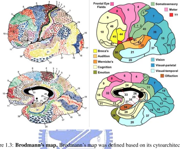
and numbered by Korbinian Brodmann based on the organization of neurons he observed in the cortex and he published his maps of cortical areas [1]. Each and every area is given a number from 1 to 52. Many of the areas have been correlated closely to diverse functions. For example, Brodmann areas 1, 2 and 3 in frontal lobe are the primary somatosensory cortex; BA 4 in frontal lobe is the primary motor cortex; BA 17 and BA 18 in occipital lobe is the primary visual cortex. Although the Brodmann areas have been discussed, de-bated, refined, and renamed exhaustively for a century, they have became the most widely known and commonly cited cytoarchitectural organization of the human cortex. Fig. 1.3 is Brodmann’s maps. Although, we know Brodmann’s map but we want to know the correct

1.1 Background 5

Figure 1.3: Brodmann’s map. Brodmann’s map was defined based on its cytoarchitecture and numbered by Korbinian Brodmann in 1909. It was divided into 52 discrete regions which was called Brodmann’s areas (BAs). Photo acquires from the web site of Professor Mark Dubin University of Colorado.

(Graphic source: http://spot.colorado.edu/ dubin/talks/brodmann/brodmann.html)

Brodmann area by using standardized x-y-z coordinates. Thus, an automated coordinate-based system to retrieve brain labels from Talairach Atlas called the Talairach Daemon is used [2]. It provided an 87 percent label match to Brodmann area labels BA 4 and BA 6 within a search range of 5 millimeters. The Talairach Atlas of human brain is defined by Talairach and Tournoux [3] in 1988. They defined a standard coordinate system on a Euro-pean female brain aged 60 by anatomizing the brain to get the exact coordinate. Therefore, we can point out that a standardized x-y-z coordinates locates on which Brodmann area. It is useful for brain tissue location and becomes an invaluable tool in modern neuroimaging.

However, postmortem-studies were one of the few ways to study brain discrepancy and the relation between behavior and the brain. It have been used to further the understanding of the brain for centuries, until the first neuroimaging technique which is called pneumoen-cephalography (PEG) is shown. The pneumoenpneumoen-cephalography, a procedure, was introduced by the American neurosurgeon Walter Dandy in 1919. With this neuroimaging technique, we can image the structure of the brain in vivo for clinical purposes or medical science. In the early 1970s, computerized axial tomography (CAT or CT scanning) was developed by Allan McLeod Cormack and Godfrey Newbold Hounsfield, and became available for di-agnostic and research purposes because of the more detailed anatomic images of the brain. Thereafter, more and more imaging technique is developed such as single photon emission computed tomography (SPECT) and positron emission tomography (PET) and the struc-tural imaging, magnetic resonance imaging like computer tomography (CT). In the next section, we will introduce magnetic resonance imaging (MRI).

1.1.2

Magnetic Resonance Imaging (MRI)

In recent years, magnetic resonance imaging (MRI) has become primarily a medical imaging technique to visualize the structure and function of the body or brain. It is also important for clinical diagnosis, medical treatment and further residential care. It was developed by Dr. Paul Lauterber in 1972 [4]. The major principle technique behind MRI is the development of nuclear magnetic resonance (NMR). In the past, magnetic resonance was used only for studying the chemical structure of substances. Until the 1970s NMR could be used to produce images of the body by Lauterbur’s and Mansfield’s great work. However, as the word nuclear was associated in the public mind with ionizing radiation exposure. It is generally now referred to simply as MRI.

There are three major components of an magnetic resonance imaging scanner : A static magnetic field, an RF transmitter and receiver, and three orthogonal, controllable magnetic gradients. Fig. 1.4 is a 3.0 T MR scanner. The image quality is directly proportional to the magnetic field strength. Higher magnetic fields increase signal-to-noise ratio, permitting higher resolution or faster scanning. However, The higher the magnetic field strength is,

1.1 Background 7

Figure 1.4: A MR scanner. Photo acquires from the web site of Research Center for Integrative Neuroimaging and Neuroinformatics (RCINN) National Yang-Ming University. (Graphic source : http://www.ym.edu.tw/rcinn/introduction.htm)

the better quality image we can acquire. A field strength of 1.0 - 1.5 T is a good compro-mise between cost and performance for general medical use. However, for certain specialist uses higher field strengths are desirable, with some hospitals now using 3.0 T scanners. Fig 1.2 is an MR image scanned by a 3.0 T MR scanner in National Yang-Ming University. With the rapid growth in MR imaging, it is a widely used technology in medical diagnosis, pathological study, and medical treatment. From head to foot, from cancer to cardiovas-cular vessel disease, from diagnosing to afterward following observations, it has already become an important imaging technique indispensable to modern medical centers.

There are many advantages of MR technology. First of all, it is noninvasive when detecting signals inside the body, so it is more safety for people under operations and diagnosis. Unlike computed tomography (CT), it uses non-ionizing radiation. Instead, it uses a powerful magnetic field to align the nuclear magnetization of hydrogen atoms in water molecules in the body. Which means MR imaging has no harm to patients who take the MR scan. Another advantage of MR imaging is that it provides much greater contrast between each different soft tissues of the body than CT does. It is especially useful in neurological (brain), musculoskeletal, cardiovascular, and oncological imaging and gives a great assistance in diagnosis of tumor or brain discrepancy in bipolar disorder (BD) or major depressive disorder (MDD). Another advantage of MR imaging is that it has no

side-effects which calls supplemental harm to patients. However, a disadvantage of MRI scanner is that the instrument is quite expensive. A new 1.5 tesla scanner approximately costs one million US dollars and two million US dollars for a new 3.0 tesla scanners. Constructing a MRI suite can cost a hundred thousand US dollars.

In human brain diagnosis and its researches, more and more studies are using CT, 2-D MR image or even higher resolution MR images. Because of the great contrast between different soft tissues of the brain, we can more easily distinguish gray matter, white matter and cerebrospinal fluid from brain. Due to the improvement of image resolution and devel-opment of the image processing tools and computers could handle numerous and complex operations, a number of unbiased whole brain morphometric analysis methods were pro-posed to characterize brain discrepancy.

1.2

Morphometrics

Morphometrics is a method to analyze the variation and the change in size or shape of organisms or brain. With the MR imaging technique, morphometric analysis are now com-monly performed on in-vivo studies and particularly useful in analyzing the fossil record. It gives a quantitative element to describe the discrepancy of objects and allows more rigor-ous comparisons. In morphometric analysis, we can describe complex shapes or variation in size, and use the numerical comparison between different objects. Furthermore, sta-tistical analysis can highlight areas where change is concentrated and quantify the level of significance. The morphometric analysis of brain images originally requires manually defining a number of regions of interest (ROI). It means that the method is based on an defined region of interests and analysis each object in this pre-defined ROI to perform the statistical differences on the volumes in each object [5].

However, the method has many potential drawbacks and limitations, including the de-mand of subject is always high, subjectivity, lacking of reproducibility. Quite a few

lim-1.2 Morphometrics 9

itations are that it is impossible to know which area in brain might be atrophy or enlarge by diseases or a surgical trauma, we could not know the relations between diseases and the area which has been analyzed by the method in advance. Although several regions are known related to the disease, the measurement may include other surrounding regions blur the results and reduces statistical power. Therefore, since a priori knowledge of regions of interest for the disease is quite important, and according to sufficient previous studies, we can make up to the deficiency of priori knowledge.

More and more complex automatically/semiautomatically morphometric methods in-clude the techniques of spatial normalization and tissue segmentation are proposed to an-alyze shape transformation or brain structure discrepancy. These methods can be divided into two categories: The first category uses the deformation fields computed by spatial normalization to compare the differences, which are to detect the differences in shape of the brain. The other category uses the normalized images to make comparisons, that is to detect the differences in brain tissue under an identical space.

The first category of morphometric method includes methods that measure the spatial transformation, which is analyzed by the deformation field deformed from templates of brain to each individual subject in the study. Several methods have been proposed, such as deformation-based morphometry (DBM) [6, 7] and tensor-based morphometry (TBM) [8, 9]. These approaches are the most direct way of measuring brain shape. But the method is based on the perfect registration between the template and the subject. Otherwise, a bad registration with small errors may reduce the accuracy of the method.

The other category of morphometric method includes the well-known method: voxel-based morphometry (VBM) [10, 11]. It uses a spatial transformation to normalize images into an identical space. Due to the use of the normalized images, the overall shape dif-ferences between subjects can be removed. It means that each subjects registered to the template will be in the same template space and in the same shape, and we can make com-parisons of brain tissue in normalized images. The method have been commonly used in several studies within the past decade.

1.3

Thesis Motivation

In this thesis, we use an multivariat approach method. The preprocessing of this ap-proach is the same with the second category of morphometric method named voxel-based morphometry (VBM). The method uses normalized images to detect differences of brain structure. Although VBM is one of the most popular morphometric method and hase been used in several studies, there are some limitations in this technique which causes VBM can not detect the differences of brain structure in a certain case: VBM detect group differences in a voxel-by-voxel manner at a time. A voxel-wise method means it consider every voxel independently to detect group differences by a statistic test, and when detecting one voxel, the neighbor voxels will be out of consideration. This voxel-wise method is simple and ease to detect every voxel independently. However, the images of the brain are shown in a 3D volume space, in the spatial point of view, the method is defectively in detecting group differences in voxel-by-voxel manner. The neighbor voxels, nearby brain tissues, should also be taken into consideration simultaneously [12].

Furthermore, in the previous section, the regions of the brain structure are always cor-related to diverse functions. For example: the frontal lobe is associated with reasoning, the parietal lobe is associated with movement, the occipital lobe is associated with visual processing, the temporal lobe is associated with perception and recognition of auditory stimuli. That is we should not consider the regions voxel-by-voxel but regions with brain structures.

In order to overcome these limitations, in this work, we proposed another method by us-ing a parcellation-based analysis approach, called the parcellation-based multivariate mor-phometry (PBM) to conquer this limitation of uni-variate analysis and of whole-brain anal-ysis. This multivariate morphometry method can take the voxles in a region into consid-eration simultaneously. In this method, a high dimensional classification technique is used and detects the most hyper-plane to separates groups. The most discriminative hyper-plane not only minimize the scatter within groups, but also maximize the scatter between groups. It can separate the different groups and characterizing the discrepancy in the regions. Also,

1.4 Related Works 11

we divide the brain into several regions in an anatomical way. The regions which are cor-related to diverse functions can be separated by the discriminative vector.

1.4

Related Works

Several Multivariate classification techniques applied to these studies typically consist of three components, feature extraction, feature dimensionality reduction and feature-based classification. Feature extraction and feature-based classification are important when ture dimensionality reduction is the next. First of all, feature extraction, When effectual fea-tures have been extract, the feature-based classification or other analysis can be completed by using several classification techniques in machine learning. Otherwise a noneffective feature will be redundant and needless for analysis. Feature dimensionality reduction is applying a mapping of the multidimensional space into a space of fewer dimensions. This means that the original feature space is transformed by applying a linear transformation such as principal components (PCA) analysis method, which is main linear technique for dimensionality reduction. PCA performs a linear mapping of the data to a lower dimen-sional space. Finally, in the field of machine learning, the goal of classification is to group subjects that have similar feature values, into groups. A linear classifier achieves this by making a classification decision based on the value of the linear combination of the fea-tures, a linear discrimination analysis technique or support vector machines (SVM)-based classifier can be used. A number of multivariate statistical classifiers have been adopted to several studies not only for classification but also for characterization of brain discrepancy. In 2002, Pettey and Geeadopted [13] proposed a multivariate linear discriminant method to characterize discrepancy of segmented MR images of the corpus callosum. At first, all segmented MR images were normalized to a male subject, and obtain for each subject a vector field or deformation field which tells us the displacement of the voxel needed to place into the correct position of the template. Finally, the quantity wishes to examine is the determinant of the jacobian of this transformation. In the pointwise statistics analysis,

they measured how different the determinant of the jacobian is between the two popula-tions. In the multivariate analysis, they chose to keep the first few principal components of the image features, to deal with the small sample size problems. Subsequently, they find the linear combination which best discriminates between the populations by applying linear discriminant analysis. The only segmented image features were used to analysis in this study.

In 2004, Lao et al. [14] proposed a support vector machine (SVM) approach method based on whole brain images. The procedures are described in the following steps: First of all, the raw images are smooth with a 3D Gaussian filter and then downsampled by a fac-tor of 4 in each dimension. Secondly, the smoothed downsampled images are segmented by using a method based on Markov random fields with inhomogeneity correction. The smoothed, downsampled and segmented images are normalized. Thirdly, they use the data of many subjects to train an SVM classifier. In the last stage, they applied the train SVM classifier to a new subject which is not including in the training set. There are two main problems in this study. One is the nonlinearity of the classifier, the other is the dimension-ality reduction before pattern classification. A nonlinear support vector classifier is used, which means the group differences depend on the morphology itself. The nonlinear SVM method can only classify the morphology data, it can not be summarized with a single im-age. Besides, the dimensionality reduction, which may be needed for dealing with a very high-dimensionality data. Due to this feature selection process, the original brain can not be reconstructed.

In 2007, Thomaz et al. [15], present a general multivariate linear framework. This is the first multivariate statistical analysis of the human brain in Alzheimer’s disease (AD) which uses the whole features simultaneously rather than segmented images. The goal is to identify and analyze the most discriminating hyper-plane separating two groups. The feature selection of the images are projected from the original space to a lower dimensional spaces by the use of Principal Component Analysis (PCA) method. Subsequently, a linear discriminant method called Maximum uncertainty Linear Discriminant Analysis (MLDA) is adopted to find the most discriminant hyper-plane on the PCA subspace.

1.5 Thesis Organization 13

It is similar to the previous work of our group [16]. Our goal is as well as to find a most discriminant vector to separate two populations by using a modified linear discrim-inant analysis method. Before the analysis of the whole brain images, we adopted a 3D wavelet transformation on the whole brain images in advance to increase spatial correla-tions between each voxels. Once we found the most discriminant hyper-plane, we perform the inverse 3D wavelet transformation to get the discriminant map in the original space. However. from our previous experiences, the voxel-based analysis somehow is defective without the consideration of nearby voxels. And in the previous work, we can figure out that the used of a modified linear discriminant method can deal with plenty of features si-multaneously. But in the whole brain analysis features may be redundant. It is superior to other multivariate methods owing to no tissue information is missing with the feature reduction processes during the multivariate analysis. Some brain regions may or may not assist the detection of group differences and some regions with a great significant level may be unimportant. A region-based approach is quite important for analyzing anatomi-cal structure. Therefore we use a parcellation-based multivariate method to analyze brain structures and detect group differences.

1.5

Thesis Organization

In the following chapters, we will introduce the voxel-based morphometry (VBM), parcellation-based multivariate morphometry (PBM), experiment results, discussion and conclusion. In chapter 2, we will introduce what VBM is, the optimized VBM protocol, the implementation of VBM and then its drawbacks. In chapter 3, we come up our idea of multivariate morphometry analysis and a framework of parcellation-based multivariate morphometry analysis. Chapter 4 is the experiment results with simulation data which is used to estimate the performance between two morphometry method. Then we have a discussion about the method and experiment results in chapter 5 and the conclusion in chapter 6.

Chapter 2

2.1

Introduction

Voxel-based morphometry (VBM) is a technique that detects the group differences in brain anatomy through a voxel-wise comparison of spatial normalized MR images [11]. That is to identify differences in relative voxels of brain structures. It is not a region of interest but whole-brain method to characterize volume and tissue concentration differences in brain structural MR images, it is also an unbiased statistical method which is a commonly used tool in the identification of characteristic differences of brain structures. By using the statistical approach of so-called statistical parametric mapping (SPM), the normalized images were statistically tested using the general linear model based on the Gaussian field theory.

In traditional morphometry method, it is based on the pre-defined regions of interest (ROI) then analyze the images with this pre-defined ROI. However, this is time consuming to define ROIs, especially when there are a large amount of subjects. And every single manual error in defining ROIs will cause small differences in volume.

VBM is increasingly applied to detect group differences in brain among various types of patient group and control groups. In recent years, it is shown that lots of the disease are correlated with the abnormal brain tissue. The method provides an analysis of inter group differences in brain tissue or volume on the voxel-wise basis in a standardized space. The results of VBM studies characterizing group differences in some disease are consistent with the result of previous studies, such as bipolar disorder (BD) [17, 18] or major depressive disorder (MDD) [18, 19].

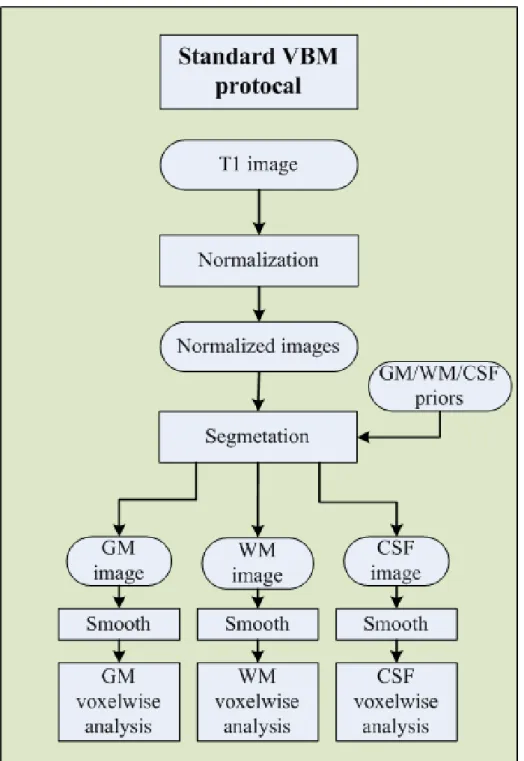
In general, the procedures of VBM analysis can be divided into two parts which are the preprocessing and the voxel-based parametric statistical analysis. Simply the procedures of the preprocessing involve spatial normalization, segmentation, and smoothing [10]. Finally, a voxel-wise statistical inference is applied to these preprocessed images. The standard VBM procedure involves four steps describe in order figure 2.1 is a standard VBM protocol.

2.1 Introduction 17

Figure 2.1: Flowchart of standard VBM protocol. Raw images are first normalized to a standard space with a template. Secondly, GM, WM and CSF are segmented from the normalized images. Thirdly, the normalized and segmented images are smoothed with an isotropic Gaussian kernel to make the data close to normal distribution. Finally, a voxel-wise statistical inference is applied to those normalized, segmented and smoothed data.

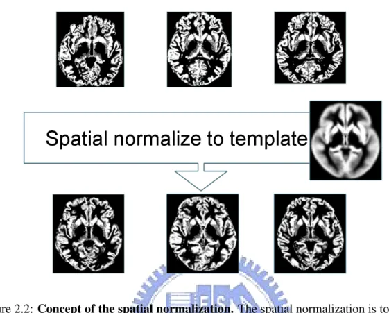
Figure 2.2: Concept of the spatial normalization. The spatial normalization is to correct the differences of shape and size between each subjects. All images in native space must be normalized to a template where the standard space is. After normalization, all voxels in the same standard space represent same tissues in each subjects.

1. Spatially normalization of all images to the same stereotactic space

As shown in the figure 2.2, the spatial normalization registers brain images of dif-ferent subjects into the same stereotactic space which is called template space. It is impossible to compare each voxel of different MR images in native space because of different sizes, shapes and the diversity of the scanning position. After spatial nor-malization, all normalized brain images are in an identical space. One certain voxel in different brain images should represent the same brain tissue. It is important that the more accurate registration we used, the fewer the choice of the template image bias the final solution.

2. GM, WM and CSF extraction from the normalized images

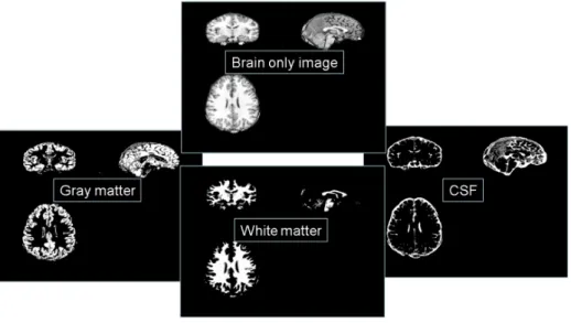
As shown in the figure 2.3, in the segmentation, the spatially normalized images are next segmented into gray matter (GM), white matter (WM) and cerebrospinal fluid

2.1 Introduction 19

Figure 2.3: The segmentation. The figure shows an example of segmentation result. A brain only image is segmented into different tissue classes which are gray matter (GM) image, white matter (WM) image and cerebrospinal fluid (CSF) image.

(CSF). After segmentation, we could obtain brain tissues and perform the statistical analysis on these tissues. In consequence of the spatial normalization and segmenta-tion, the voxel at the same position represents the same brain tissue.

3. Smoothing

In smoothing, the segmented gray and white matter images are now smoothed by convolving with an isotropic Gaussian kernel. The size of the smoothing kernel should be comparable to the size of the expected regional differences between the groups of brains, but most studies have employed a 12 millimeter FWHM kernel. It makes the data more normally distributed and reduces the registration error which is resulted from spatial normalization. It also ensures that each voxel in the images contains the average amount of gray or white matter tissue around the voxel.

4. Voxel-based statistical analysis for localization

As a result of the smoothing step, a VBM analysis involves a voxel-wise statistical analysis by comparing the normalized and smoothed GM or/and WM images of dif-ferent groups of subjects. Standard parametric statistical procedures (t tests) are used

to test the hypotheses at each and every voxel, to measure the group difference is to find out the area or voxels reach the significant level in statistic two sample t test. The results comprise the level of group differences and if reaching the significant level, we can say that there is a difference between the groups at this voxel. Eventually, A voxel-wise statistical parametric map (SPM) comprises the result of many statistical tests.

There are various ways to implement voxel-based morphometric methods. The purpose of different implementation is to maximize the ability of making inferences in group differ-ences. For example, another method applied the procedure in the order: segmentation first, normalization, smoothing and statistical analysis which is called RAVENS [5] method. In the next section, we will introduce another improvement method based on the standard VBM called optimized VBM [10].

2.2

Optimized VBM Protocol

There are several studies reveal potential problems of the standard VBM. One of those studies discusses about the imperfect registration effects on VBM. An imperfect registra-tion may cause the segmentaregistra-tion error because of brain tissue is in the different space, and it leads into an incorrect comparison between normal control and patient subject [20]. It is owing to the implementation of segmentation. In the segmentation method, a mixture model technique is used, and the model contains the distributions of the voxel intensity of brain tissues (GM, WM, CSF). A priori probability map contains a priori knowledge of the distribution of the brain tissues in normalized space is used to improve the segmentation of brain tissues. Furthermore, if the VBM analysis is focus on the brain tissues such as gray matter or white matter, the segmented image will be normalize into template space which may cause that, the better segmented images used the better accuracy of the registration. In conclusion, the registration and segmentation influences each other, an optimized VBM protocol is proposed by Good et al. [10].

2.2 Optimized VBM Protocol 21

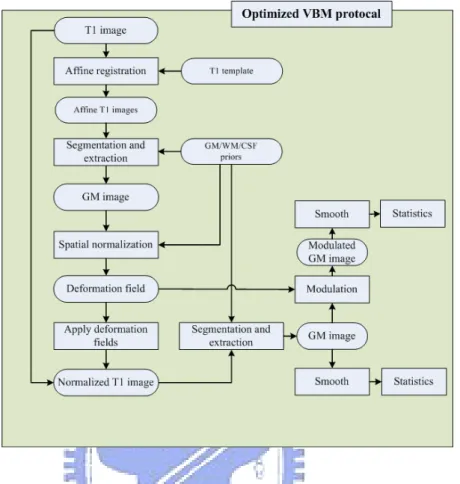
Figure 2.4: Flowchart of optimized VBM protocol. Optimized VBM protocol consists of the following seven steps: (1) creation of GM, WM and T1 template, (2) segmentation and extraction of affine-registered brain images, (3) normalization of GM/WM/CSF images into the GM/WM/CSF template, (4) normalization of whole brain T1 images with optimized normalization parameters, (5) segmentation and extraction of normalized T1 images, (6) modulation, and (7) smoothing.

The optimized VBM protocol [10] for characterizing group differences of gray or white matter is list below in order, and Fig 2.4 is the flowchart of optimized VBM protocol.

1. Creation of GM, WM, CSF and T1 template

Customized template is created by averaging all the normalized smoothed gray/white matter subjects from the standard VBM protocol. the optimized template is created to minimize any potential bias for spatial normalization. All T1 images are normalized to a template, segmented into GM, WM and CSF images and then smoothed with an 12 millimeter full-width at half-maximum (FWHM) isotropic Gaussian kernel.

Each normalized, segmented and smoothed T1/GM/WM/CSF images are averaged to create T1/GM/WM/CSF templates respectively.

2. Segmentation and extraction of affine-registered brain images

This is a fully automated method to remove scalp tissue, skull and non-brain tissues. At first, all T1 images in native space are segmented into GM, WM and CSF images. Then a series of morphological operations is applied to these segmented images to re-move unconnected non-brain voxels. Finally the gray and white matter are extracted in native space.

3. Normalization of GM/WM/CSF images into the GM/WM/CSF template

In this step, the segmented GM/WM/CSF images in native space are normalized to the customized GM/WM/CSF template individually in stereotactic space. Thus we can obtaining the optimal deformation fields.

4. Normalization of whole brain T1 images with optimized normalization param-eters

The optimal deformation fields obtained in the previous step are now reapplied to the raw whole brain T1 images in native space. Therefore we can obtain the raw T1 images which are in the same space with the gray/white matter template.

5. Segmentation and extraction of normalized whole brain images

In order to get a preferable segmentation, the optimally normalized whole brain Ti images are now in the stereotactic space. Then segmented into gray, white matter and CSF. A series of morphological operations is applied again to these segmented images to remove unconnected non-brain voxels. Finally, the optimally normalized and segmented GM/WM/CSF images are got in stereotactic space.

6. Correction for volume changes which is also calle modulation step (optional) Due to the nonlinear spatial normalization, volumes of certain brain areas may be enlarge or atrophy. In order to preserve the volume of a certain region within a voxel, a correction for volume changes, usually called as modulation. A multiplying voxel values in the segmented images by the Jacobian determinants which is obtained in

2.2 Optimized VBM Protocol 23

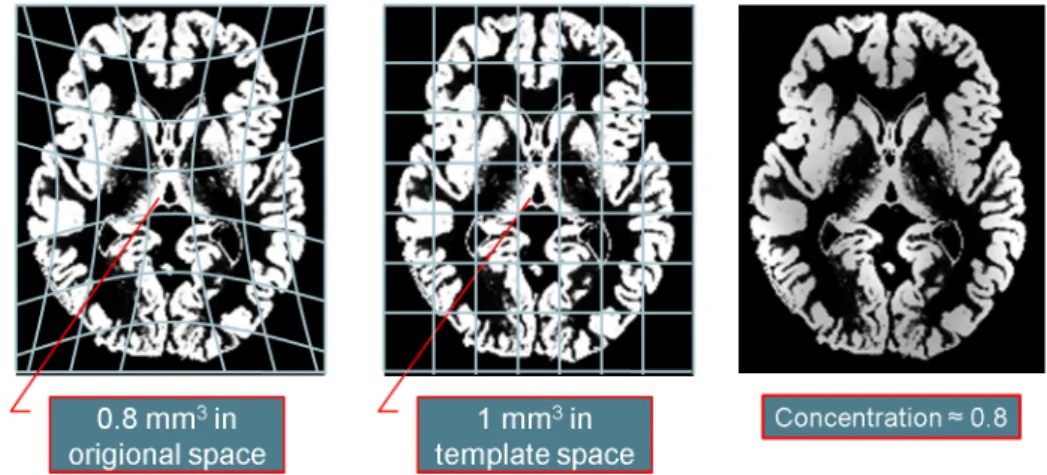
Figure 2.5: Concept of the modulation. The figure illustrates the modulation of a normal-ized segmented image. Due to the spatial normalization, after images are normalnormal-ized into a standard space, volumes of certain brain areas may be enlarge or atrophy. The result of modulation are used to correct for volume changes. For example, the pixel in the native space is 1 millimeter square. after normalization, the pixel becomes 3 millimeter square in standard space. It means, the concentration should be divided by 3 to preserve total volumes in each pixels.

the spatial normalization step. Figure 2.5 is a concept of the modulation. 7. Smoothing

It is same with the standard VBM method, the optimally normalized segmented and modulated images of different tissues are smoothed using an isotropic Gaussian ker-nel. Smoothing makes the population more normally distributed and reduces the registration error. The choice of the smoothing kernel is related to the expected dif-ferences. An 8 millimeter or 12 millimeter FWHM smoothing kernel is often used in VBM method.

8. Statistical analysis

As the standard VBM method, a voxel-wise statistical analysis is performed on those optimally normalized, segmented, modulated and smoothed images to characterize regionally discrepancy between different groups. The use of two-sample t test is to calculate the significance of group differences at every voxel. The t-test map is a 3D volume, the voxel dimension and voxel size which are the same with every MR

images. Thus we can make inferences in group differences by each voxel which is stored in t test map reaches a significance level.

The optimized VBM protocol provides a more preferable normalization and segmen-tation. And features of the optimized VBM are first creating a separated grey and white matter templates, and second a fully automatic brain extraction technique. It also adopts a modulation step to preserve volume change during spatial normalization.

2.3

Implementation of VBM

In order to maximize the ability of making inferences in group differences, an imperfect registration and a bad segmentation result will reduce the ability of the VBM, which implies that each of steps in VBM is important and each bad results may affect the VBM studies badly. Therefore we should be careful when implementing every single step and make sure that the performance of tools we used is the best. Several tools are used in VBM studies such as brain extraction, segmentation and spatial normalization. Following is the implementation of VBM by our group.

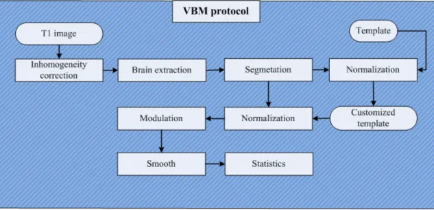
The implementation of VBM in this work is illustrated in figure 2.6. It is similar with standard VBM protocol but in different order of the normalization and the segmentation step, due to the characteristic of the segmentation tool which can segment images in the native space instead of a standard space. Moreover the bias correction is done at first to correct the inhomogeneity of the magnetic field which may cause the image tissues become difficult to differentiate.

1. Bias correction with N3

An artifact often seen in MRI is for the signal intensity to vary smoothly across an image, which is referred to as RF inhomogeneity or intensity non-uniformity. It is

2.3 Implementation of VBM 25

Figure 2.6: Flowchart of VBM implementation. Our implementation of VBM uses sev-eral tools and can be described in eight steps: (1) Bias correction, (2) non-brain exclusion of T1 images with HWA, (3) segmentation and extraction of brain T1 images with FAST, (4) normalization of segmented GM, WM and CSF images, (5) creation of customized GM, WM and CSF templates, (6) normalization of segmented GM, WM and CSF images to customized template, (7) correction for volume changes, (8) smoothing and voxel-based morphometric statistical analysis.

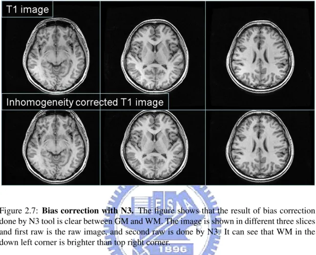
usually due to poor radio frequency (RF) field uniformity. Raw images is first cor-rected by nonparametric nonuniform intensity normalization (N3) [21] which is a non-parametric method for correction of intensity non-uniformity in MRI data and minimize the within-class variance of GM, WM and CSF. Bias correction will also improve the image quality for segmentation. Figure 2.7 is an example of bias correc-tion.

2. Non-brain exclusion of T1 images with HWA

The T1 corrected images is secondly skull-stripped using a hybrid watershed algo-rithm (HWA) [22].Hybrid Watershed algoalgo-rithm is a relatively more sensitive tool that often results in a conservative strip that rarely removes any brain tissue. It is an fully automatic, robust and efficiently algorithm which removes non-brain tissue, and does not unduly influence the outcome. All images are segmented to remove

Figure 2.7: Bias correction with N3. The figure shows that the result of bias correction done by N3 tool is clear between GM and WM. The image is shown in different three slices and first raw is the raw image, and second raw is done by N3. It can see that WM in the down left corner is brighter than top right corner.

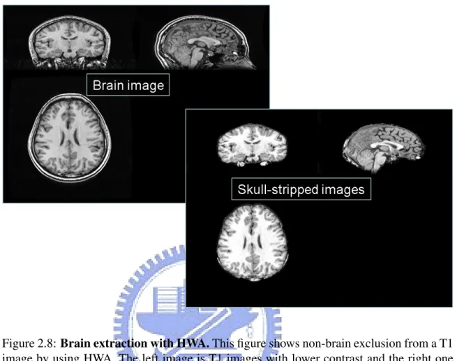
non-brain parts in native space with HWA. The default parameters were utilized for automated processing. On average, HWA required less than 8 min of processing time per dataset. Figure 2.8 is an example of non-brain exclusion.

3. Segmentation and extraction of brain T1 images with FAST

All T1 inhomogeneity corrected images without non-brain tissues derived from the previous step are segmented into GM, WM and CSF images in native space with FMRIB’s Automated Segmentation Tool (FAST) in FSL. Its method is based on a hidden Markov random field model and an associated Expectation-Maximization al-gorithm [23, 24]. The value of a voxel in segmented images represents a probability of belonging to one particular tissue, ranged from 0 to 1. We use this probability to represent the tissue volume of the segmented images.

2.3 Implementation of VBM 27

Figure 2.8: Brain extraction with HWA. This figure shows non-brain exclusion from a T1 image by using HWA. The left image is T1 images with lower contrast and the right one is an extracted brain image without non-brain materials after segmentation by HWA. The quality of the extracted image has been improved and would make a good segmentation with FAST.

4. Normalization of segmented GM, WM and CSF images

All segmented GM, WM and CSF images are respectively normalized to a template by first an affine-registration and follow a nonlinear registration [25].

5. Creation of customized GM, WM and CSF templates

All segmented normalized GM, WM and CSF images are in a standard space and av-eraged to create customized GM, WM and CSF templates. The customized templates are more close to the population sample of the study and minimize the distortion caused by normalization in later processes.

The segmented GM, WM and CSF images in native space obtained in third step are independently normalized to the corresponding GM, WM and CSF customized templates obtained from the previous step. Then all segmented and normalized GM/WM/CSF images of different subjects are now in the same space that is the voxel in the same position will stand for the same tissue. Moreover, during the nor-malization of the deformation field are stored in order to correct volume changes in next step.

7. Correction for volume changes (modulation)

Due to the nonlinear spatial normalization, the volumes of certain brain areas may be enlarge or atrophy. In order to preserve the volume of a certain region within a voxel, a correction for volume changes, usually called as modulation. A multiplying voxel values in the segmented and normalized images by the Jacobian determinants which is obtained in the spatial normalization step. In our analysis, these modulated images are used to analyze the volume discrepancy between different groups. 8. Smoothing and voxel-based morphometric statistical analysis

The segmented, normalized and modulated images are smoothed to be close to nor-mal distribution by sing an isotropic Gaussian kernel, and an 12mm FWHM smooth-ing kernel is used. Then, a voxel-wise statistical analysis is performed on these seg-mented, normalized, modulated and smoothed GM/WM/CSF images to characterize regionally discrepancy between different groups. The use of two-sample t test is to calculate the significance of group differences at every voxel. Then a 3D volume with t-test map is stored to make inferences in group differences.

In this work, we applied preprocessing of the VBM protocol to deal with MR im-ages. We maintain concepts of the VBM protocol and implement it with N3 (IDeA Lab, UC Davis Center for Neuroscience), HWA (FreeSurfer, http://surfer.nmr.mgh.harvard.edu), FSL (Analysis Group, FMRIB, Oxford, UK), SPM2 softwares in Matlab 7.0 (the Math-Works, Inc. Natick, MA, USA).

2.4 Drawbacks of VBM 29

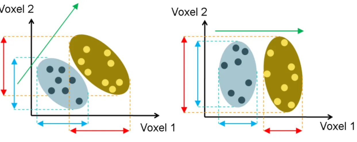
Figure 2.9: Schematic scatterplots illustrating of significant bias of VBM. There are two ellipse which stands for two different morphological groups. For example, one is normal control group the other is affected group. In the right case, there is no overlay along the voxel 1 axis. it is easy for VBM to detect group difference depending at the voxel 1 even with a small number of samples, but detect no difference at the voxel 2. In the left case, VBM may fail to find group difference along each axis because of the high overlay. This is a significant bias of VBM analysis which is very limited in detecting group differences.

2.4

Drawbacks of VBM

Each of subjects can form a person’s morphological profile by collecting voxel-wise morphological measurements which is consist of every voxel in volume data. These mea-surements can be placed into a high-dimensional space, each dimension representing a voxel. That is, if spatial normalization is perfect, we can say that each voxel in differ-ent MR image stands for the same tissue, the oridiffer-entation of group differences in a high-dimensional space consists of every voxel in a MR image. Then the group differences are then reflected by the degree of separation of the respective morphological profiles. Fig-ure 2.9 is a schematic scatterplots in two dimension. The normal morphological profiles and the affected morphological profiles will form two distributions in two-dimension space. The dimensionality of the space is much higher and equal to the number of voxels being interrogated, but here we use 2D examples for display purposes.

the data in an bias way, it is fundamentally limited in making inference of group differ-ences. Two cases are shown in figure 2.9. The orientation of group differences in a high-dimensional space in practice, here in our case, 2-high-dimensional space is used. Owing to the voxel-based morphometry analysis detect group differences in a voxel-wise manner, VBM considers only one dimension at a time. That is on the right of figure 2.9, in which the group difference will be detected along dimension 1 (voxel 1), even with very small number of samples. Because there is a significant difference at voxel 1. VBM may de-tect no group difference along voxel 2. In another case, on the left of figure 2.9, VBM may detect no group difference along each axis because diseased and normal groups might have different means, but the overlap is high. This is a significant bias of VBM analysis which is very limited in detecting group differences. In summary, the two cases, show that voxel-based morphometry analysis will detect group differences easily at one axis in morphological profile. However, the dimension in MR images is always high and there are subtle and complex differences in brain structures, may not be easy for VBM to detect the significance of group differences.

Although voxel-based morphometry analysis in group differences is of great worth. But the bias of VBM limits the power of detecting subtle and complex structures. This bias is an fundamental limitation of voxel-based morphometry, because the ways of VBM in de-tecting group differences is voxel-by-voxel manner rather than the consideration of nearby voxels or several structures in brain. In the above two cases, it is clear that there is a group different between two distribution at voxel 1 and voxel 2. If two voxels are in considera-tion, It is easy to differentiate between two different distribution of morphological profiles. That is the more voxels we consider, the more subtle or complex structures we may detect. Therefore, in this thesis, we proposed another unbiased method using a region-based multi-variate analysis approach which is also automatic to overcome this fundamental limitation.

Chapter 3

Parcellation-Based Multivariate

Morphometry

3.1

Introduction

According to the drawbacks of voxel-based morphometry analysis method, we use a multivariate morphometry analysis method which characterizing the group differences of brain structures. The multivariate morphometry method is an unbiased method that we can compare voxels in a multivariate manner to overcome the drawbacks of voxel-based morphometry analysis. Before the multivariate analysis is adopted, the preprocessing of the raw MR images is also similar with VBM analysis. The main difference of this thesis is the multivariate analysis.

In multivariate analysis, all voxels in MR images are features simultaneously taken into consideration in a high-dimensional space. The more voxels this multivariate method analysis the higher dimension it forms. The goal of the multivariate analysis is to detect the most discriminative hyper-plane which separates the two different groups in the high-dimensional space. That is the most discriminative hyper-plane is a linear combination of features which best separate two or more groups of MR images. Each features are projected onto this discriminative hyper-plane which best separates two different groups. Further, each parameters of this discriminative vector is a weight which stands for the discrimina-tion of each dimensions, features or voxels. That means, once we find a discriminative projection vector, each weights of the vector is a discrimination of characterizing group differences and it is also an image called discriminant map. The discriminant map can be visualized to identify the location in brain.

From the previous work of our group [16], a multivariate whole brain analysis is pro-posed. The use of whole brain images and linear multivariate classification technique demonstrated that the method has a good sensitivity to subtle and complex brain struc-tural differences. Somehow, taking all features into consideration may be redundant in our experience. And voxel-based analysis method which considers only one voxel at a time without nearby voxels is also a drawbacks. Thus a parcellation-based approach is needed.

The concept of the parcellation-based analysis method is proposed. That every voxel in the same regions are taken into account simultaneously for characterizing group differences

3.2 Framework of Parcellation-Based Multivariate Morphometry 33

in each regions. The brain will be parcellated into several different regions especially based on brain structures. The interaction of every voxel in the same region can be sufficiently an-alyzed by a multivariate method. The relation between disease and brain structures is quite close but the relation between disease and undefined-regions is relatively small. Moreover, several voxels or predefined regions which are more important in characterizing in group differences can be taken into consideration if they were known in advanced. In brief, the related information of each voxel in same regions are in consideration, it contradicts to the voxel-based morphometry analysis in characterizing group discrepancy.

In consequence, a parcellation-based multivariate morphometry method is proposed for characterizing differences of brain structures. we can quantified differences of each regions through the parcellation-based manner by a linear multivariate classification technique in a high-dimensional space.

3.2

Framework of Parcellation-Based Multivariate

Mor-phometry

The procedure of parcellation-based multivariate morphometry is similar with voxel-based morphometry. The first seven steps of the implementation of voxel-voxel-based morphom-etry is used. The preprocessing includes bias correction, brain extraction, segmentation, normalization, template creation, normalization to customized template and modulation. Smoothing step is not included because of the subtle differences of brain structures may be reduced by smoothing data, more details will be listed in chapter 5, discussion. After the preprocessing, the segmented, normalized and modulated gray/white matter images are all in the same space. Subsequently, parcellation-based multivariate morphometry analysis will be adopted to find group differences of brain structures.

The parcellation-based multivariate morphometry analysis can be divided into three parts. First of all, we extract regions of brain by Anatomical Automatic Labeling (AAL)

Figure 3.1: Schematic of the Anatomical Automatic Labeling template. The AAL tem-plate is in three different views which is obtained in MRIcroN software. An official site for Anatomical Automatic Labeling (AAL) freeware: http://www.cyceron.fr/freeware/

which is a software package and digital atlas of the human brain [26]. The definition of 45 anatomical volumes of interest (AVOI) in each hemisphere were delineated with the Mon-treal Neurological Institute (MNI) single-subject main sulci. The procedure was performed using a dedicated software which allowed a 3D following of the sulci on the brain. Re-gions of interest were then drawn manually with the same software every 2 millimeter on the axial slices of the high-resolution MNI single subject figure 3.1 is a schematic of AAL template. There are 116 regions defined by AAL and all of the regions will be extracted by using this AAL template.

Secondly, the main part of the multivariate analysis, each of the regions will adopt a modified LDA-based method, the discriminative common vector method [27] to find the most discriminant projection vector. It is simultaneously minimizes the scatter within each individual group and maximizes the scatter between groups without the small sample size problem. The resulting projection vector forms a spatial map, whose image size is the same with each regions, containing the regions which are most representative of group differences. That is, each parameters of this discriminative projection vector is a represen-tative of the discrimination of each groups, features or voxels. Details of the method will be interpreted in the next section.

Thirdly, combining each regions back into original brain, the resulting projection vec-tor containing the most representative of group differences of each extracted regions. It

3.2 Framework of Parcellation-Based Multivariate Morphometry 35

Figure 3.2: Concept of the relation between projection vector with each standard bases.

is a most discriminant map of each regions that the weight of each feature represents the degree of importance for characterizing group differences. The resulting projection vector will form an angle with each standard basis. The angle Θi is computed by the formula

Θi = arccos_|PPlda· ˆei

lda|| ˆei|. Where Pldais the projection vector and ˆeiis the standard basis. That

is each of the weight wi is the same with cos Θi. Even the weights are in different regions

we can combine them all together. Figure 3.2 is the concept of the relation between projec-tion vector and each standard basis. Before we combine each parameters of the resulting projection vectors back into original brain, there will be a problem of representing the de-gree of importance for characterizing group differences. The resulting projection vector will be a unit vector which is computed by modified linear discriminant method. The more dimension the unit vector has, the smaller parameters it gets with the same atrophy. The correction is done before combining each results. Details of the method of the combina-tion of each results will also be interpreted in the next seccombina-tion. After the combinacombina-tion, we will get the most discriminant projection vector of two different groups. The weight of projection vector represents the degree of importance for characterizing group differences. Finally, for the purpose of displaying each regions of the significance level which is the weight of the discriminant map. There are two map we will illustrate. One is the t map

of each regions the other is weights of the discriminant map itself. A t-test map is calcu-lated by projecting all the subject onto the projection vector. That is a high-dimensional space reduce to an one dimensional space, a value, which represent a subject from different groups. A two-sample t test is adopted to these values to calculate t value of each regions. That means, we can obtain a whole brain confidence to demonstrate the significance level of each regions by calculating T-statistic. Each voxel in the same regions will have same t statistic value. Once we know the important regions by T-statistic value, we may be in-terested not only in the regions we found but also the more precise location of this region. Therefore, weights of the discriminant map is shown with a smoothing and thresholding (optional). Each parameter of the discriminating map denotes the discrimination of charac-terizing the group discrepancy, the changes of the weight of neighboring parameters should be slight. However, in practice, it does not often look smooth because of the error produced during the preprocessing of a bad image registration or tissue segmentation or because of the noise or the variation within groups. Some errors may be produced by an imperfect image registration. To overcome these problems, the smoothness is used with a 6 millime-ter FWHM gaussian kernel. The smoothing and thresholding are used for visualization of discriminant map to show the location of the group differences.

In summary, the parcelation-based multivariate morphometry contains the following steps:

1. Bias correction of T1 images 2. Brain extraction

3. Segmentation of the brain only images into GM, WM, and CSF 4. Spatial normalization of all images to the same stereotactic space 5. Creation of customized template

6. Spatial normalization of all segmented images to the customized template space 7. Modulation

3.3 Multivariate Analysis using a Modified LDA-Based Method 37

8. Multivariate analysis

(a) Extraction of regions of brain

(b) Discriminative common vector method to obtain the most discriminant projec-tion vector

(c) Combination of resulting discriminant projection vector 9. Visualization of the discrepancy pattern

(a) Smoothing (b) Thresholding

Figure 3.3 is the flowchart of the parcellation-based multivariate analysis without the preprocessing steps. In the following sections we will introduce the techniques used in the multivariate analysis step, including the discriminative common vector method and the combination method of resulting discriminative common vector.

3.3

Multivariate Analysis using a Modified LDA-Based Method

3.3.1

Conventional Linear Discriminant Analysis and Its Potential

Prob-lem

Fisher’s Linear discriminant analysis (LDA) is one of the most popular linear classi-fication techniques which is invented in 1936 and the methods has been used in statistics and machine learning to find the linear combination of features which best separate two or more classes of objects or events. The objective of this method is to find the most discriminant projection vector P, in which different groups can be separated with the max-imum between-class scatter matrix and the minmax-imum within-class scatter matrix. The most projection matrix Plda that maximizes the Fisher’s linear discriminant criterion, which is

Figure 3.3: Flowchart of parcellation-based multivariate analysis. After the preprocess-ing, in the parcellation-based multivariate analysis we first extract the regions of brain, and then we apply the discriminative common vector method to each region and the correction is done before combination. Finally, we combine all the results of every region in brain back to original brain.