犯罪與經濟誘因: 以美國州資料1970-2000為例

犯罪與經濟誘因: 以美國州資料 1970-2000 為例

研究成果報告(精簡版)

中 華 民 國 96 年 09 月 14 日

Does Unemployment Increase Crime? Evidence from

1974-2000 US State Data

Ming-Jen Lin

Abstract

OLS may understate the effect of unemployment on crime because of the endogeneity problem (Raphael and Winter-Ember 2001). In this paper, we use changes in the real exchange rate, state manufacturing sector percentage and state union membership rates as novel instrumental variables to carry out 2SLS estimations. We find a 1 percentage point increase in unemployment would increase property crime by 1.8 percent under the OLS method, but that the elasticity goes up to 4 percent under 2SLS. The larger 2SLS effect has significant policy implications since it explains 30 percent of the property crime change during the 1990s.

Keywords: Crime; Unemployment; Instrumental variables; Real exchange rate.

JEL Code: K4.

* _{Ming-Jen Lin is an associate professor at the Department of Economics, National Taiwan University. The}

author thanks Steven Levitt, David Mustard, Tom Miles, Mark Duggan, and two anonymous referees for their help comments. Financial support from National Science Council, Taiwan is greatly acknowledged. The data used in this article can be obtained beginning August 2007 through July 2010 from Ming-Jen Lin, Department of Economics, National Taiwan University, [email protected].

I. Introduction

Crime imposes enormous economic costs on society,1 with unemployment also being thought to have an important role to play in the supply function of crime.2 The coincidence between the longest economic expansion since World War II and the overall reduction in crime rates in

the 1990s seems to confirm this argument. Between 1991 and 2000, there was a significant

fall in the annual unemployment rate in the US, from 6.8 percent to 4.8 percent. Furthermore,

as noted by Levitt (2004), according to calculations based upon the ‘Uniform Crime Report’

(UCR), over the same period, there were considerable reductions in acts of murder (-42.9

percent), violent crime (-33.6 percent) and property crime (-28.8 percent). Such a strong

correlation provides policymakers with confirmation that reducing the level of unemployment

is one of the most effective ways of fighting crime.

Economists typically conclude that unemployment (or a decline in labor market

conditions) can lead to an increase in crime, because the worsening opportunities in the legal

employment sectors make committing crime more attractive (Becker 1968). And such

propensity is expected to have more relevance to property crime because of its pecuniary

nature (Levitt 2004). In terms of empirical evidence, recent studies reach consensus that

unemployment does have a positive, significant, but only small effect on property crime, and

unemployment increases property crime by 1.0 to 2.0 percent (Freeman 1995; Bushway and

Reuter 2002; Levitt 2004). This trend is seen more clearly when, as opposed to the average

unemployment rate, better measures are used to identify those who are on the margin of

committing crime.3

This paper contributes to the existing knowledge in this area by providing a better means

of identifying the causal link between labor market conditions and crime. We focus on

breaking down the endogeneity between unemployment and crime, and on how the policy

implications of the magnitude of the 2SLS estimations differ from those in the prior literature

obtained under OLS estimations. Adopting US state panel data, we use changes in the

exchange rate, state union membership percentage and state manufacturing percentage as

novel instrumental variables in unemployment, and find that although a 1.0 percentage point

increase in unemployment would increase property crime by 1.8 percent under OLS

estimation, this elasticity goes up to between 4.0 and 6.0 percent under the 2SLS method. We

also confirm that unemployment has no significant effect on violent crime.

Our results contribute to the existing literature in three ways. First of all, and quite

surprisingly, although the more recent studies have shown that changes in labor market

conditions can affect property crime with regard to those who are more likely to be on the

Levitt (2001), when using panel data, the instrumental variable approach is a preferable means

of identifying the link between crime and unemployment, since simultaneity, omitted

variables and measurement error can all lead to bias in the OLS results. To the best of our

knowledge, only Raphael and Winter-Ember (2001) and Gould, Weinberg, and Mustard (2002)

attempt to explore the instrumental variable (IV) method, although the measures they obtained

are quite different.5

Given that our 2SLS estimates are twice the size of the OLS estimates, this also confirms

the suspicions of Raphael and Winter-Ember (2001), that the available evidence understates

the effects of unemployment on crime.6 The 2SLS results obtained in this study consequently contribute to the literature by better controlling for endogeneity, and thereby providing more

precise estimations than those reported in the prior literature.

Secondly, the magnitude of our 2SLS estimations also points to very different policy

implications than may have previously been considered. As opposed to the traditional results of

1.0 to 2.0 percent under the OLS method, there is a two- to three-fold increase in the 2SLS

estimates of the effect of unemployment on property crime, rising to about 4.0-6.0 percent. This

indicates that the 2 percentage point reduction in unemployment in the 1990s would reduce

property crime by between 8.0 and 12.0 percent. This would also explain about 33 percent of the

effect of the legalization of abortion (Levitt and Donohue 2001). However, if, as suggested in the

prior OLS literature, elasticity is only 1.0-2.0 percent, then unemployment may have only a minor

role to play, if any role at all, in the reduction in crime in the 1990s (Levitt 2004).

Finally, although the recent literature shows that average unemployment may not be an

appropriate measure – in terms of identifying those who are at the financial margins of

committing crime – our results show that such a positive effect can still be identified if

endogeneity is properly controlled. This may be because the variations picked up in the

present study through the IV method are for those people working in manufacturing who are

thus more likely to be substituted by foreign competition. 8 Our study adds support to the growing opinion within the literature that, when better measures are obtained, there is

increasing evidence of labor market conditions affecting crime.

The remainder of this paper is organized as follows. Section 2 reviews the extant literature,

followed in Section 3 by a description of the data and a discussion of the identification problem.

The empirical results are presented in Section 4, where we justify the use of the instruments by

building up a causal link between exchange rate fluctuations, union membership and

unemployment. We then undertake a comparison of the 2SLS and OLS results in Section 5, and

Section 6 concludes.

The theoretical approach to the ways in which economic incentives affect criminal behavior

can be seen in Becker (1968), Ehrlich (1973) and various later works. When unemployment,

the opportunity cost of committing a crime, namely, the legal wage, declined, which makes

illegal income more appealing. A graphic version of this argument can also be seen in

Grogger (2000) and Raphael and Winter-Ember (2001). This prediction is also likely to be

more relevant for property crime which leads to direct financial gain (Levitt 2004).

As to the empirical evidence, the early studies on the positive effect of unemployment on

crime are described as ‘inconsistent, insignificant and weak’ (Chiricos 1987). Furthermore,

there is surprisingly little evidence to support the proposition that crime rates are driven by

economic conditions (Piehl 1998); this has, however, changed over the past ten years, with the

more recent articles consistently reporting the positive, significant and small effects of

unemployment on property crime, but not on violent crime.

Using the OLS method and US panel data on states, counties and cities, a number of

studies find that a 1 percentage point increase in the unemployment rate increases property

crime by just 1.0 to 2.0 percent.9 Using time series data on New York City, Corman and Mocan (2005) finds that elasticity was about 1.8-2.2 percent for only burglary and motor theft,

while Papps and Winkelmann (2002) also finds the elasticity of unemployment on property

Spengler (2000) calculates that the elasticity of unemployment on total crime in Germany is

around just 0.5 percent.10

Such significant changes can be attributed to three factors. Firstly, the recent studies are

better at identifying the more relevant variables, since the average unemployment or wage

measures may not be appropriate, in terms of identifying those on the margin of committing

crime. From their focus on young, unskilled and low-educated males, Gould, Weinberg, and

Mustard (2002) finds that a 1.0 percentage point increases in the unemployment rate of this

‘at-risk’ group would increase property crime by only 1.0 to 2.0 percent. Machin and Meghir

(2004) also found strong evidence to support the effect on crime from conditions in the

low-wage labor market.11 The second factor for consideration is recognition of the need for controlling the potential problems caused by endogeneity; however, to the best of our

knowledge, only Raphael and Winter-Ember (2001) and Gould, Weinberg, and Mustard (2002)

make such attempts by using 2SLS. The third factor is that we are now at a much better stage

in terms of extensively controlling for the independent variables, as well as in the usage of

panel data, given that the periods under examination are now much longer.

The overall picture from the above literature and many of the survey articles is that

unemployment has a small, positive and significant effect (of about 1.0 to 2.0 percent) on

which does not control for endogeneity. In the only two studies which adopt the use of

instrumental variables, the magnitude of the effects obtained, and hence the policy

implications, are very different.12

This research therefore sets out to add to the literature by using a set of novel instruments

as the means of solving the rarely-discussed problem of endogeneity, and by discussing the

differences in the estimations, as well as their impact on crime policy.

III. The Data and the Problem of Identification III-A. The Data

The data used in this paper comprise of a panel of 49 US states with observations covering the

period from 1974 to 2000.13 Following Levitt (1996), seven crime categories from the UCR are included. These are: murder, rape, assault and robbery, collectively referred to as ‘violent

crime’, and burglary, larceny and auto theft, collectively referred to as ‘property crime’. The

overall numbers of local and state police forces are also listed in the UCR.

The total number of prisoners and details on the use of the death penalty are obtained

from the Criminal Justice Statistics Source Book produced by the Bureau of Justice, while the

figures for the total consumption of ethanol per person are taken from the website of the

economic incentive variables, which include state income per capita, hourly wages,

unemployment rates, state public aid, health and education expenditure, the proportions of

metropolitan and African-Americans, poverty levels, age structure and the AFDC (TANF) per

recipient family per year, are taken from various issues of the Statistical Abstract of the

United States.

As to the instrumental variables, the real exchange rates are taken from the historical data

archives at the Federal Reserve Bank of New York, and the oil price series can be found in the

Annual Energy Review published by the Department of Energy within the US Central

Government. The percentages of employees in manufacturing, manufacturing value and union

membership are also taken from various issues of the Statistical Abstract of the United States.

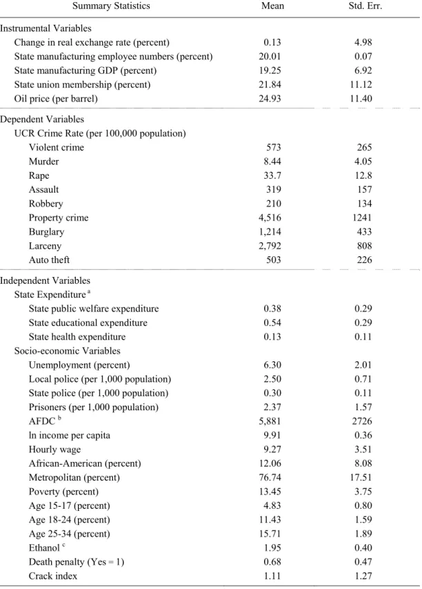
The summary statistics provided in Table 1 show that between 1974 and 2000, there

were approximately 5,000 crimes committed each year for every 100,000 persons in the US,

albeit relatively minor property crimes in the great majority of cases. The table also shows that

there were approximately 237 prisoners, 250 local police and 30 state police per 100,000 of

the population. The average state expenditure per capita per year was $380 on public welfare,

$540 on education and $130 on health, while the average hourly wage was $9.76.

Approximately 76 percent of the population lived in urban areas, with African-Americans

<Table 1 is inserted about here>

As to the key variables, the average unemployment rate was 6.30 percent and the price of

oil was $24.93 per barrel. The manufacturing sector accounted, on average, for 20.01 percent

of state total employees and 19.25 percent of all state GDP, with 21.8 percent of the workers

holding union membership at state level.

III-B. The Problem of Identification

In general, there are three factors which can explain bias in the OLS results, the first of which

is the problem of omitted variables. If, for example, any pro-cyclical crime-related commodity

consumption is omitted, then the OLS method would underestimate the true effects (Raphael

and Winter-Ember 2001).14 _{Cook and Zarkin (1985) suggests that legitimate employment}

opportunities, criminal opportunities, crime-related commodities and the responses by the

criminal justice system are all important variables in the crime supply function. In this paper,

we use unemployment rates, state income per capita, hourly wages and poverty rates as

independent variables to represent the economic incentive factors. Special attention should be

paid to hourly wage and poverty rates, since wages and the economic conditions of lower

percentile workers are very important to the determination of crime (Grogger 1998; Gould,

Other control variables include state education, public aid and health expenditure

(government spending), prisoner and police numbers,16 the death penalty (deterrence), alcohol (crime-related goods), age structure and metropolitan percentages. To further control for

unobserved variables that do not follow a specific trend or that do not change overtime, we

add in state, year and state-specific linear and quadratic trends as control variables to fully

explore the advantages of our state panel data.17 Although it is not possible to prove that all the relevant independent variables have been included in the specifications, our main

conclusions hold, both with and without state trend dummies, and also remain insensitive to

the inclusion or exclusion of particular control variables.

The second possible explanation for bias in OLS estimations is the problem of

simultaneity between crime and unemployment. The overall effect of unemployment may be

underestimated under OLS if criminal activity reduces the employability of offenders

(Raphael and Winter-Ember 2001) or if crime increases unemployment as a result of the flight

of employers (Cullen and Levitt 1999). The third explanation is that the OLS method would

underestimate the effect if there is random measurement error in unemployment.

Overall, as noted by Raphael and Winter-Ember (2001), omitted variables and

simultaneity lead to some suspicion that the available evidence understates the effect of

unemployment on property crime being both positive and consistently larger than the OLS

estimates, and indeed, this is the major finding in our empirical results section.

IV. Empirical Results

IV-A. OLS Regression Results

In the first instance, we report the OLS results as a reference point under the following

specifications:

ln (Crime ijt) = ρUnemployment it + βXit + φi

(1)

+ Year t + φi*Year t + φi*Year t2

+ξijt

where the dependent variables are different crime rates, j indicates the crime category, i is

state, t is year, Xit represents all the independent variables outlined earlier in Table 1, φi and

Year t represent state and year dummies, and the final two terms are state specific linear and

quadratic linear trends.

For each crime category, we present three different specifications by gradually adding in

linear and quadratic linear trends. The results are presented in Table 2.

<Table 2 is inserted about here>

are positive and significant at the 99 percent level. When state and year dummies and other

independent variables are added, the elasticity is 0.026, or 2.6 percent. After adding in the

linear and quadratic linear trends, the respective estimates become 1.1 percent and 1.8

percent. It is clear, therefore, that unemployment has a positive and significant, but

relatively small, effect on property crime. However, its effects on violent crime are

insignificant since economic incentives often play a much smaller role in violent crime

vis-à-vis property crime.

Alcohol consumption is positively related to violent crime, and we also find that more

prisoners, more police, higher per capita income, the death penalty and fewer young people all

result in crime reduction. Overall, the standard specification shows that a 1.0 percentage point

increase in unemployment can increase property crime by around 1.1 to 1.8 percent, although

it has no significant impact on violent crime. This result is similar to those reported in the

prior literature.

IV-B. Instrumental Variables and the First Stage Results

As noted earlier, the OLS results may contain bias stemming from omitted variables,

simultaneity or simple measurement error. To obtain a consistent estimator, we need to find an

two conditions for a valid IV are relevance, namely Cov (Z, Unemployment)≠0, and

exogeneity, Cov (Z, μ)=0. According to Levitt (1997) and Angrist and Krueger (2001), the

three criteria that must be met are: (i) detailed knowledge of the economic mechanisms and

institutions for the instrumental variables selected; (ii) an over-identification test if there are

more IVs than endogenous variables; and (iii) a weak IV test.

In this paper, we use the changes in the real exchange rate between adjacent years,

RERCt = 1 -t 1 t RER RER

RER − _t− _{, multiplied by the percentage of state manufacturing sector}

employees or GDP value (that is, RERCit=RERCt*Manufacturing percentit) to instrument

unemployment. It should be noted that the real exchange rate (RER) is calculated by the

average foreign exchange rates of all trade partners weighted by trade volume. By weighting

the manufacturing employee percentage, we can measure the specific RERC shock (dollar

appreciation or depreciation) to which each state is exposed in any given year. This is the

strategy adopted by Raphael and Winter-Ember (2001), in which oil costs are used as the

instrumental variable.

The effects of exchange rate movement and unemployment, particularly in the

manufacturing sector, are well documented in the prior literature. As argued by Revenga

(1992), the link between dollar appreciation and industry employment is ‘straightforward’,

tend to shift employment in the same direction. In theory, currency appreciation can affect the

domestic labor market by altering profit (Sheets, 1992; Clarida 1997), investment (Campa and

Goldberg 1999) or production location (Goldberg 1993). As to the prior empirical estimations,

Branson and Love (1988) finds that the US manufacturing sector lost over one million jobs as

a direct result of the 1981-1985 appreciation of the US dollar.

Using industry level manufacturing sector data covering the period between 1977 and

1987, Revenga (1992) finds that import prices appeared to have a sizable effect on

employment. A number of other studies also reports that most of the adjustments to an adverse

trade shock came through employment.18 In addition, since exchange rate equilibrium is determined in the global money market, although the US is a relatively large economy within

that market, it is unlikely that any state-specific unemployment rate change (the variation used

in our 2SLS estimations) would affect overall US exchange rates.

Furthermore, using macro-level variables as instruments for micro-level decisions is not

uncommon within the literature (see for example, Evans and Ringel 1999; Currie and Moretti

2003); however, there is a need to take into account whether exchange rates are correlated

with certain omitted variables which may affect crime, but which may not have been

controlled within the regression. To mitigate this issue, we control for the economic variables

each of which may be correlated with exchange rate shocks, and which may also affect crime

rates. We also include state, year and trend dummy variables to identify those variables that

are not included in the independent variables. Of course, the list cannot be exhaustive, and we

acknowledge the possible pitfall in our analysis here.

In addition to using the percentage of state employees and the percentage of GDP

accounted for by the manufacturing sector, we also use the percentage of state union

membership as our weighting for real exchange rate movements. As noted by Freeman and

Medoff (1984), unions are simply “organizations [that] have monopoly power which they can

use to raise wages above competitive levels”. As a consequence, an excess supply of labor is

created due to the deviation from the competitive market equilibrium, resulting in

unemployment.19

We have so far introduced three weighting methods, the percentage of state

manufacturing sector employees, the percentage of state manufacturing sector GDP and the

percentage of state union membership, as the real exchange rate change variables. We also

add in oil price (weighted by these three variables) as the instrumental variables for

comparison with Raphael and Winter-Ember (2001). The justification for the impact of oil

shocks on unemployment can be seen in Davis and Haltiwanger (1999), in which they

We can now begin our 2SLS analysis. In the first stage we run:

Unemployment it = σIVit + βXit + φi + Year t

(2)

+ φi*Year t + φi*Year t2

+ ξit

where Xit refers to all of the state expenditure and social economic variables used in equation (1).

Our instrumental variables are the two macroeconomic variables weighted by the three different

procedures: (i) RERC*state manufacturing sector employee percent; (ii) RERC * state

manufacturing sector GDP percent; (iii) RERC * state union membership percent; (iv) Oil price *

state manufacturing sector employees percent; (v) Oil price * state manufacturing sector GDP

percent; and (vi) Oil price * state union membership percent. Once the first stage results are

obtained, the predicted value of unemployment will replace the observed unemployment rates in

stage 2, namely, Equation (3):

ln (Crimeijt) = ρUnemployment it + βXit + φi + Year t

(3) + φi*Year t +φi*Year t2 +ξijt

Table 3 presents the first stage results using real exchange rate movements. The positive

and highly significant coefficient estimates indicate that dollar appreciation, along with

manufacturing and union membership percentages, are positively correlated with the

<Table 3 is inserted about here>

By carrying out a simple calculation, we can determine whether our estimation results

are comparable with those of the earlier studies. We know that from 1980-1985, there was

appreciation of about 33 percent in the real exchange rate, and, as column (1) of Table 3

indicates, the coefficient estimate of RERCt*manufacturing employee t-1 percent is 54, which

means that the unemployment rate increase due to this appreciation would be 55*0.33 (dollar

appreciation)* 0.2(mean of manufacturing employee percent)=3.63 percent, or roughly four

million unemployed people. This number is similar to the 4.0-7.5 percent unemployment

estimated by Revenga (1992).

We also use state manufacturing percentage (GDP or employee numbers) plus union

membership as a set of instrumental variables for the first stage when subsequently carrying

out the over-identification test, with both the sign and significance of the coefficient estimates

all fitting our prediction. Furthermore, as argued by Bound, Jaeger, and Baker (1995), Staiger

and Stock (1997) and Stock and Yogo (2004), the first stage joint F test value should be large

enough to pass the weak IV tests. Table 3 shows that the F-statistics for the null hypothesis,

namely that all of the coefficient estimates of the instrumental variables in the first stage

regression are not jointly different from zero, range from 21 to 58, significantly larger than the

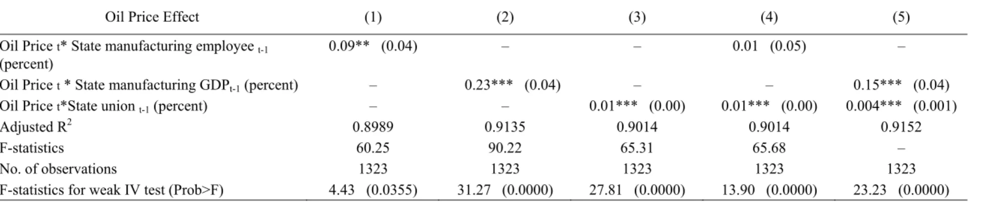
For the purpose of comparison, oil prices weighted by the three different methods are

also used as instrumental variables. It should be noted that we do not put oil price and

exchange rate together because these two variables have high collinearity. The procedure is

the same as that in Table 3. The results, which are presented in Table 4, indicate that oil price

shocks weighted by manufacturing or union percentages lead to an increase in the

unemployment rate; the weak IV test is also passed, with the single exception of column (1).

<Table 4 is inserted about here>

IV-C. 2SLS Regression Results

The final step in the 2SLS regression is to enter the predicted value of the unemployment rates

obtained from Equation (2) into our second stage regression, namely Equation (3). We first

use ‘Real exchange rate change * state manufacturing employees percent’ to perform a single

IV 2SLS regression. To test the sensitivity of the model specifications, we report the

regression results by gradually adding in the state specific linear trend and quadratic trend

dummy variables. The results are reported in Table 5.

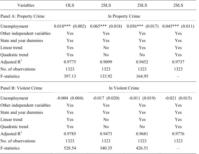
<Table 5 is inserted about here>

As we can see, the OLS estimation of the elasticity of unemployment on property crime

range between 4.4 and 6.5 percent, consistently greater than the OLS results, and dependent

on whether or not state specific linear or quadratic trends are included. Unemployment

appears to have no significant effect on violent crime, in both the OLS and 2SLS estimations.

To further investigate this issue, we first use the six instrumental variables to obtain the

first stage prediction value of unemployment. We then use all seven UCR crime categories

(murder, rape, assault, robbery, burglary, larceny and auto theft) as the dependent variables to

perform a single IV 2SLS regression using the full model specifications of Equation (3). The

results are presented in Table 6.

<Table 6 is inserted about here>

It is clear that for property crime, the 2SLS estimations of unemployment elasticity for

the six different single instrumental variables range between 2.5 and 5.5 percent, much greater

than the OLS estimation (1.6 percent). Furthermore, the ranges of the respective 2SLS results

for the property crime category (burglary, larceny and auto theft) were 2.1-6.6 percent, 1.6-5.4

percent and 4.1-15.8 percent. These are consistently greater than the OLS results (2.5 percent,

1.1 percent and 1.7 percent). The unemployment effect on violence is also insignificant,

except for its negative relationship with rape (strong) and murder (much weaker).

perform an over-identification test. This can be carried out by regressing the predicted residuals

of the 2SLS on all of the exogenous and instrumental variables, and then calculating the χ2 value

of n (the number of observations) x R2. The results presented in Table 7 show that, with the

exception of larceny, all of the crime categories pass the over-identification test, with most of

the statistics being less than 2. This indicates that the 2SLS method remains insensitive to the

instrumental variables chosen.

<Table 7 is inserted about here>

As to the estimation of unemployment elasticity, it is also clear that the 2SLS method

produces 2.9-5.4 percent for property crime, 3.0-6.7 percent for burglary, 2.5-5.0 percent for

larceny and 4.7-8.0 percent for auto theft. Again the effects of unemployment on violent crime

are unclear, with the exception of the negative effects for both rape and murder. These

numbers are similar to the single IV results presented in Table 6, and also similar to those

reported by Raphael and Winter-Ember (2001).

So far, we show a greater effect of unemployment on property crime under the 2SLS

method than under the OLS method. However, we can find no significant effect of

unemployment on violent crime. Our results also pass the first stage weak IV test and the

however, several issues in need of further attention; these are discussed in the following

section.

V. Discussion

The first issue of importance is the negative sign of unemployment on violent crime, although

some of them are insignificant. In some model specifications, unemployment also has a

significant negative effect on murder (weak) and rape (very strong). Although unemployment

can basically increase property crime, the negative correlation between unemployment and

violent crime is not immediately obvious from the theory. Furthermore, the positive effect of

unemployment on robbery is also generally weak, which is somewhat strange, since the

motivation for committing robbery, namely, economic gain, is similar to that for property

crime. We offer two alternatives for reconciliation of this point.

Firstly, the overall unemployment rate may not be capable of identifying those people

who are on the margin of committing a particular crime, even after controlling for

endogeneity. For example, since almost all rape offenders are male, the gender specific

unemployment rate should be a better measurement than the overall unemployment rate.

Indeed, Raphael and Winter-Ember (2001) shows that while overall unemployment has a

when the male unemployment rate is used.

Secondly, as pointed out by Raphael and Winter-Ember (2001), the failure to control for

crime-related commodity variables, such as alcohol, guns and drugs, each of which

demonstrate pro-cyclical pressure, can lead to underestimation of the true effects of

unemployment. Levitt (2004) also argued that since most crime-related commodities, such as

alcohol and cocaine, were normal goods, improvements in economic conditions can have a

negative impact on crime. It is likely that the reason we obtain a negative unemployment

effect on violent crime is because we do not control variables which are pro-cyclical and have

particularly profound effects on violent behavior; cocaine appears to be one of them.20 To explore this point further, we include the ‘state crack cocaine index’ calculated by

Fryer et al. (2005) – which includes data from 1980 to 2000 only – as a control variable into

all of our OLS and 2SLS regressions. The process is essentially the same as those outlined in

Equations (2) and (3). The results presented in Table 8 show that when adding in the crack

index and using data from 1980 to 2000, the effect of unemployment on violent crime

(including both murder and robbery) becomes positive (although not significant). Furthermore,

the estimates of unemployment on robbery are about 5.0 to 7.0 percent under the 2SLS

method, which is similar to the effect on property crime. This shows when a proper measure

violent crime becomes positive, small and insignificant. Nevertheless, the positive, significant,

and larger estimates of unemployment on property crime under the 2SLS method remain.

<Table 8 is inserted about here>

Finally, we also attempt to introduce as many combinations of the independent variables

as possible, and find that the results are not at all sensitive to the inclusion or exclusion of any

particular controls; that is, unemployment has a significantly positive effect on property crime,

with the magnitude of the effect larger under the 2SLS methods. Nevertheless, one might

suspect that it may be the employment conditions among certain particular demographic

groups that drive our results. This direction may well be worthy of further investigation if

more detailed data were to become available.21

IV. Conclusions

Obtaining a precise measure of the impact of unemployment on crime is very important,

insofar as it facilitates a cost benefit analysis for the assessment of possible public policy

interventions. Although economic theories predict that unemployment should have a positive

effect on property crime, most of the prior literature has reported that a 1.0 percentage point

increase in the unemployment rate is associated with a 1.0 percent increase in property crime,

method, which does not control for endogeneity.

In this paper, we begin with a discussion of the ways in which the problems of omitted

variables and simultaneity can lead to bias in the OSL estimations. We control for an

extensive set of independent variables, including deterrence, economic conditions,

demographics, year and state dummies, and state-specific linear and quadratic trends, so as to

mitigate the problem of omitted variables. We then use a set of novel instrumental variables,

namely changes in the real exchange rate, state union membership percentage, oil price and

state manufacturing employee percentages to mitigate the problem of simultaneity.

Our first stage regression shows that appreciation in the US dollar and in oil prices,

together with union membership and manufacturing employee percentages, have a strong

positive effect on unemployment. Furthermore, the results of the first stage easily pass the

weak IV test. In the second stage analysis, we show that the 2SLS estimation of the elasticity

of unemployment on property crime is 4.0 to 6.0 percent for the full model specifications, as

compared to the 1.8 percent obtained under the OLS method. The fact that the 2SLS results

are consistently greater than those obtained under the OLS method indicates that the two

major sources of bias stemming from the OLS method are the positive response of

unemployment to the problem of crime, and the omitted variables which cause crime, but

As for violent crime, there is no apparent significant effect attributable to unemployment,

in either the OLS or 2SLS estimations. We also use the over-identification test in an attempt

to reveal the sensitivity of the choice of instrumental variables; however, with the single

exception of larceny, all of the 2SLS results hold. Finally, our results remain insensitive to

both the different model specifications and the choice of independent variables.

The 4.0 to 6.0 percent estimates obtained in this study on the effect of unemployment on

property crime have important policy implications, since they indicate that roughly one-third

of the reduction in property crime during the 1990s may have been attributable to changes in

unemployment, a conclusion that is very different to those drawn in much of the prior

References

Anderson, David. 1999. “The Aggregate Burden of Crime.” Journal of Law and Economics

42(2): 611-42.

Angrist, Joshua, and Alan Krueger. 2001. “Instrumental Variables and the Search for

Identification: From Supply and Demand to Natural Experiment.” Journal of Economic

Perspective 15(4): 69-85.

Becker, Gary. 1968. “Crime and Punishment: An Economic Approach.” Journal of Political

Economy 76(2): 169–217.

Belman, Dale, and Thea Lee. 1995. “International Trade and the Performance of US Labor

Markets.” In US Trade Policy and Global Growth, ed. Robert Blecker, 61-107. Armonk,

New York: ME Sharpe.

Blumstein, Alfred, and Richard Rosenfeld. 1998. “Explaining Recent Trends in US Homicide

Rates.” Journal of Criminal Law and Criminology 88(1): 1175-216.

Branson, William, and James Love. 1988. “United States Manufacturing and the Real

Exchange Rate.” In Misalignment of Exchange Rates: Effects on Trade and Industry, ed.

Bound, John, David Jaeger, and Regina Baker. 1995. “Problems with Instrumental Variables

Estimation when the Correlation between the Instruments and the Endogenous

Explanatory Variable is Weak.” Journal of the American Statistical Association 90(430):

443-50.

Burgess, Simon, and Michael Knetter. 1998. “An International Comparison of Employment

Adjustment to Exchange Rate Fluctuations.” Review of International Economics 6(1):

151-63.

Bushway, Shawn, and Peter Reuter. 2002. “Labor Market and Crime.” In Crime: Public

Policies for Crime Control, James Wilson, and Joan Petersilia, eds. San Francisco, CA: ICS Press.

Campa, Jose, and Linda Goldberg. 1999. “Investment, Pass-through and Exchange Rates: A

Cross-Country Comparison.” International Economic Review 40(2): 287-314.

__________. 2001. “Employment versus Wage Adjustment and the US Dollar.” Review of

Economics and Statistics 83(3): 477-89.

Chiricos, Theodore. 1987. “Rates of Crime and Unemployment: An Analysis of Aggregate

Clarida, Richard. 1997. “The Real Exchange Rate and US Manufacturing Profits: A

Theoretical Framework with Some Empirical Support.” International Journal of Finance

and Economics 2(3): 177-88.

Cook, Philip, and Gary Zarkin. 1985. “Crime and the Business Cycle.” Journal of Legal

Studies 14(1): 115-28.

Corman, Hope, and Naci Mocan. 2005. “Carrots, Sticks and Broken Windows.” Journal of

Law and Economics 48(1): 235-66.

Cullen, Julie, and Steven Levitt. 1999. “Crimes, Urban Flight and the Consequences for

Cities.” Review of Economics and Statistics 81(2): 159-69.

Currie, Janet, and Enrico Moretti. 2003. “Mother’s Education and the Intergenerational

Transmission of Human Capital: Evidence from College Opening.” Quarterly Journal of

Economics 118(4): 1495-532.

Davis, Steven, and John Haltiwanger. 1999. ” NBER Working Paper No.7095. Cambridge,

MA: National Bureau for Economic Research.

Donziger, Steven. 1996. The Real War on Crime. New York: Harper Collins.

of Economics 116(2): 379-420.

Ehrlich, Isaac. 1973. “Participation in Illegitimate Activities: A Theoretical and Empirical

Investigation.” Journal of Political Economy 81(3): 521-65.

Entorf, Horst, and Hannes Spengler. 2000. “Socioeconomic and Demographic Factors of

Crime in Germany: Evidence from Panel Data of the German States.” International

Review of Law and Economics 20(1): 75-106.

Evans, William, and Jeanne Ringel. 1999. “Can Higher Cigarette Taxes Improve Birth

Outcomes?” Journal of Public Economics 72(1): 135-54.

Friedberg, Leora. 1997. “Did Unilateral Divorce Raise Divorce Rates? Evidences from Panel

Data.” American Economic Review 88(3): 608-27.

Freeman, Richard. 1995. “The Labor Market.” In Crime, James Wilson, and Joan Petersilia,

eds. San Francisco, CA: ICS Press, 171-92.

Freeman, Richard, and Morris. Kleiner. 1990. “The Impact of New Unionization on Wages

and Working Conditions.” Journal of Labor Economics 8(1), Part 2: S8-S25.

Fryer, Richard, Paul Heaton, Steven Levitt, and Kevin Murphy. 2005. “Measuring the Impact

of Crack Cocaine.” NBER Working Papers No.11318. Cambridge, MA: National Bureau

of Economic Research.

Goldberg, Linda. 1993. “Exchange Rates and Investment in United States Industry.” Review

of Economics and Statistics 75(4): 575-88.

Goldberg, Linda, and Joseph Tracy. 2000. “Exchange Rates and Local Labor Markets.” In The

Impact of International Trade on Wages, ed. Robert Feenstra. Chicago, Ill: University of Chicago Press.

Gould, Eric, Bruce Weinberg, and David Mustard. 2002. “Crime Rate and Local Labor

Market Opportunities in the US: 1979-1997.” Review of Economics and Statistics 84(1):

45-61.

Gourinchas, Pierre. 1998. “Exchange Rates, Job Creation and Job Destruction.” In NBER

Macroeconomics Annual, Ben Bernanke, and Julio Rotemberg, eds. Cambridge, MA: MIT Press.

Grogger, Jeff. 1998. “Market Wage and Youth Crime.” Journal of Labor Economics 16(4):

__________. 2000. “An Economic Model of Recent Trends in Violent Crime.” In The Crime

Drop in America, Alfred Blumstein, and Joel Wallman, eds. Cambridge, MA: Cambridge University Press, 266-87.

Grogger, Jeff, and Michael Willis. 2000. “The Emergence of Crack Cocaine and the Rise in

Urban Crime Rates.” Review of Economics and Statistics 82(4): 519-29.

Jarrell, Stephen, and T. D. Stanley. 1990. “A Meta-analysis of the Union/Non-union Wage

Gap.” Industrial and Labor Relation Review 44(1): 54-67.

Kletzer, Lori. 2000. “Trade and Job Losses in US Manufacturing, 1979-1994.” In The Impact

of International Trade on Wages, ed. Robert Feenstra. Chicago, Ill: University of

Chicago Press.

Layard, Richard, and Steven Nickell. 1986. “Unemployment in Britain.” Economica

53(Supplement): S121-170.

Lewis, Gregg. 1985. Union Relative Wage Effect. Chicago, Ill: University of Chicago Press.

Levitt, Steven. 1996. “The Effect of Prison Population Size on Crime Rate: Evidence From

Prison Overcrowding Litigation.” Quarterly Journal of Economics 111(2): 319-51.

on Crime.” American Economic Review 87(3): 270-90.

__________. 1998. “Juvenile Crime and Punishment.” Journal of Political Economy 106(6):

1156-85.

__________. 2001. “Alternative Strategies for Identifying the Link between Unemployment

and Crime.” Journal of Quantitative Criminology 17(4): 377-90.

__________. 2004. “Understanding Why Crime Fell in the 1990s: Four Factors that Explain the

Decline and Six that Do Not.” Journal of Economic Perspective 18(1): 163-90.

Lin, Ming-Jen. 2006. “Does Unemployment Increase Crime? Evidence from County Data of

Taiwan 1978-2003 (In Chinese).” Taiwan Economic Review 34(4): 445-483.

Linneman, Peter, Michael Wachter, and William Carter. 1990. “Evaluating the Evidence on

Union Employment and Wages.” Industrial and Labor Relations Review 44(1): 34-53.

Marvell, Thomas, and Carlisle Moddy. 1996. “Police Levels, Crime Rates and Specification

Problems” Criminology 24(3): 606-46.

Meghir, Costas, and Steve Machin. 2004. “Crime and Economic Incentives.” Journal of

Miller, Ted, Mark Cohen, and Brian Wiersema. 1996. “Victim Costs and Consequences: A

New Look.” National Institute of Justice Research Report, NCJ-155282, available at

website: http://www.ncjrs.org/pdffiles/victcost.pdf.

Papps, Kerry, and Rainer Winkelmann. 2002. “Unemployment and Crime: New Evidence for

an Old Question.” New Zealand Economic Papers 34(2): 53-72.

Piehl, Anne. 1998. “Economic Conditions, Work and Crime.” In Handbook of Crime and

Punishment, ed. Michael Thorny. New York: Oxford University Press.

Piehl, Anne, and Kristin Butcher. 1998. “Cross-city Evidence on the Relationship between

Immigration and Crime.” Journal of Policy Analysis and Management 17(3): 457-93.

Raphael, Steven, and Rudolf Winter-Ember. 2001. “Identifying the Effect of Unemployment

on Crime.” Journal of Law and Economics 44(1): 259-83.

Revenga, Ana. 1992. “Exporting Jobs? The Impact of Import Competition on Employment

and Wages in US Manufacturing.” Quarterly Journal of Economics 107(1): 255-84.

Ruhm, Cristopher. 1995. “Economic Conditions and Alcohol Problems.” Journal of Health

Economics 14(5): 583-603.

115(2): 617-750

Sheets, Nathan. 1992. “The Exchange Rate and Profit in Developed Economies: An

Inter-sectoral Analysis.” Working paper, Board of Governors of the Federal Reserve System.

Stock, James, and Douglas Staiger. 1997. “Instrumental Variables Regression with Weak

Instruments.” Econometrica 65(3): 557-86.

Stock, James, and Mark Watson. 2003. Introduction to Econometrics, Addison-Wesley,

348-372.

Stock James, and Yogo Motohiro. 2004. “Testing for Weak instruments in Linear IV

Regression?” In Identification and Inference in Econometric Models: Essays in Honor of

Thomas J. Rothenberg, Donald Andrews, and James Stock, eds. Cambridge: Cambridge University Press.

US Department of Energy, Annual Energy Review (various issues), available at website:

Table 1 Summary statistics, weighted by population, 1974-2000

Summary Statistics Mean Std. Err.

Instrumental Variables

Change in real exchange rate (percent) 0.13 4.98 State manufacturing employee numbers (percent) 20.01 0.07

State manufacturing GDP (percent) 19.25 6.92

State union membership (percent) 21.84 11.12

Oil price (per barrel) 24.93 11.40

Dependent Variables

UCR Crime Rate (per 100,000 population)

Violent crime 573 265 Murder 8.44 4.05 Rape 33.7 12.8 Assault 319 157 Robbery 210 134 Property crime 4,516 1241 Burglary 1,214 433 Larceny 2,792 808 Auto theft 503 226 Independent Variables State Expenditure a

State public welfare expenditure 0.38 0.29

State educational expenditure 0.54 0.29

State health expenditure 0.13 0.11

Socio-economic Variables

Unemployment (percent) 6.30 2.01

Local police (per 1,000 population) 2.50 0.71 State police (per 1,000 population) 0.30 0.11

Prisoners (per 1,000 population) 2.37 1.57

AFDC b _{5,881 2726}

ln income per capita 9.91 0.36

Hourly wage 9.27 3.51 African-American (percent) 12.06 8.08 Metropolitan (percent) 76.74 17.51 Poverty (percent) 13.45 3.75 Age 15-17 (percent) 4.83 0.80 Age 18-24 (percent) 11.43 1.59 Age 25-34 (percent) 15.71 1.89 Ethanol c _{1.95 0.40}

Death penalty (Yes = 1) 0.68 0.47

Notes:

a _{State education expenditure, state public welfare expenditure and state health expenditure are US$1,000 per capita, and} are adjusted by the CPI.

b _{AFDC is per recipient family per year (TANF after 1997).} c _{Ethanol is gallons consumed per capita per year.}

Table 2 OLS results of unemployment and state demographic variables on property and violent crime, 1974-2000 a

Variables _{Coefficient Std. Err. Coefficient Std. Err. Coefficient Std. Err.}

Panel A: Property Crime ln Property Crime b

Unemployment 0.026*** 0.003 0.011*** 0.002 0.018*** 0.002

ln Income per capita -0.533*** 0.106 -0.441*** 0.131 -0.199** 0.097

ln Hourly wage 0.130** 0.066 0.093 0.061 0.000 0.019

ln Local police rate t-1 -0.047 0.039 -0.149*** 0.043 -0.049 0.032

ln State police rate t-1 -0.005 0.008 -0.002 0.003 -0.001 0.002

ln Prisoner rate t-1 -0.210*** 0.018 -0.180*** 0.021 -0.130*** 0.020

ln AFDC (or TANF) 0.031 0.022 0.009 0.017 0.025 0.018

Poverty Rate (percent) -0.010*** 0.002 -0.004 0.001 0.000 0.001

Metropolitan (percent) 0.001*** 0.000 0.001** 0.000 0.001** 0.000

African-American (percent) 0.961 0.612 3.203*** 0.963 -3.186*** 1.115

ln Ethanol per capita 0.938*** 0.071 0.037 0.085 -0.145** 0.072

ln State education expenditure 0.070*** 0.025 0.119*** 0.028 0.004 0.017

ln State public expenditure 0.040** 0.019 -0.012 0.022 0.012 0.019

ln State health expenditure 0.011 0.010 0.007 0.007 0.002 0.004

Age 15-24 (percent) 3.035*** 0.598 4.303*** 0.593 2.089*** 0.717

Age 25-34 (percent) 3.409*** 0.540 5.580*** 0.707 3.653*** 0.772

Death Penalty -0.096*** 0.017 -0.069*** 0.017 -0.035*** 0.013

State and year dummies Yes Yes Yes

Linear trend dummies No Yes Yes

Quadratic trend dummies No No Yes

F statistics 199.49 264.43 397.13

Adjusted R2 _{0.9280 0.9618 0.9775}

Table 2 (Contd.)

Variables Coefficient Std. Err. Coefficient Std. Err. Coefficient Std. Err.

Panel B: Violent Crime ln Violent Crime b

Unemployment 0.005 0.004 -0.007** 0.004 -0.004 0.003

ln Income per capita -0.227 0.171 -0.188 0.166 -0.065 0.142

ln Hourly wage -0.263 0.198 0.076 0.048 0.013 0.042

ln Local police rate t-1 -0.051 0.048 -0.131*** 0.050 -0.012 0.047

ln State police rate t-1 0.018* 0.010 0.001 0.005 0.003 0.004

ln Prisoner rate t-1 -0.091*** 0.023 -0.143*** 0.029 -0.131*** 0.027

ln AFDC (or TANF) -0.024 0.033 -0.036 0.033 -0.032 0.030

Poverty Rate (percent) 0.001 0.003 -0.004* 0.002 0.002 0.002

Metropolitan (percent) 0.001 0.001 0.000 0.001 -0.000 0.000

African-American (percent) -1.939*** 0.794 2.155 1.832 -3.060 2.253

ln Ethanol per capita 0.766*** 0.102 0.426*** 0.029 0.331*** 0.127

ln State education expenditure -0.001 0.041 0.071* 0.038 -0.097*** 0.030

ln State public expenditure 0.010 0.026 0.048 0.029 0.035 0.027

ln State health expenditure 0.043*** 0.014 0.016** 0.009 0.012* 0.008

Age 15-24 (percent) 2.863*** 0.700 3.974*** 0.869 2.257* 1.296

Age 25-34 (percent) 6.703*** 0.872 6.508*** 1.154 4.874*** 1.099

Death Penalty -0.134*** 0.028 -0.083*** 0.022 -0.095*** 0.022

State and Year Dummies Yes Yes Yes

Linear Trend Dummies No Yes Yes

Quadratic Trend Dummies No No Yes

F statistics 346.97 434.69 528.54

Adjusted R2 _{0.9496 0.9685 0.9785}

No. of observations 1323 1323 1323

Notes:

a _{Regressions are weighted by population.}

Table 3 First stage results of the effect of changes in real exchange rates on unemployment a,b

Real Exchange Rate Changes (RERC) (1) (2) (3) (4) (5)

RERCt* State manufacturing employee t-1

(percent) 53.96*** (8.64) – – 22.00*** (8.64) –

RERCt* State manufacturing GDP t-1 (percent) – 47.49*** (7.90) – – 26.53** (8.47)

RERCt* State union t-1 (percent) – – 1.37*** (0.18) 1.15*** (0.19) 0.78*** (0.19)

Adjusted R2 _{0.9065 9288 0.9103 0.9108 0.9246}

F-statistics 63.54 63.39 68.33 68.59 69.40

No. of observations 1323 1323 1323 1323 1323

F-statistics for Weak IV test (Prob>F) 39.00 (0.0000) 36.07 (0.0000) 58.43 (0.0000) 30.95 (0.0000) 20.95 (0.0000)

Notes:

a _{Standard errors are in parentheses.}

Table 4 First stage results of the effect of oil price on unemployment

Oil Price Effect (1) (2) (3) (4) (5)

Oil Price t* State manufacturing employee t-1

(percent)

0.09** (0.04) – – 0.01 (0.05) –

Oil Price t * State manufacturing GDPt-1 (percent) – 0.23*** (0.04) – – 0.15*** (0.04)

Oil Price t*State union t-1 (percent) – – 0.01*** (0.00) 0.01*** (0.00) 0.004*** (0.001)

Adjusted R2 _{0.8989 0.9135 0.9014 0.9014 0.9152}

F-statistics 60.25 90.22 65.31 65.68 –

No. of observations 1323 1323 1323 1323 1323

F-statistics for weak IV test (Prob>F) 4.43 (0.0355) 31.27 (0.0000) 27.81 (0.0000) 13.90 (0.0000) 23.23 (0.0000)

Notes:

a _{Standard errors are in parentheses.}

Table 5 OLS and 2SLS results of the effect of unemployment on property and violent crime

Variables OLS 2SLS 2SLS 2SLS

Panel A: Property Crime ln Property Crime

Unemployment 0.018*** (0.002) 0.065*** (0.018) 0.056*** (0.017) 0.045*** (0.011)

Other independent variables Yes Yes Yes Yes

State and year dummies Yes Yes Yes Yes

Linear trend Yes No Yes Yes

Quadratic trend Yes No No Yes

Adjusted R2 _{0.9775 0.9099 0.9452 0.9737}

No. of observations 1323 1323 1323 1323

F-statistics 397.13 133.92 164.95 –

Panel B: Violent Crime ln Violent Crime

Unemployment -0.004 (0.004) -0.017 (0.020) -0.011 (0.019) -0.021 (0.015)

Other independent variables Yes Yes Yes Yes

State and year dummies Yes Yes Yes Yes

Linear trend Yes No Yes Yes

Quadratic trend Yes No No Yes

Adjusted R2 _{0.9785 0.9473 0.9681 0.9776}

No. of observations 1323 1323 1323 1323

F-statistics 528.54 340.35 426.51 –

Notes:

a _{The instrumental variable is ‘Real Exchange Rate Change*State manufacturing employees percentage’; standard errors}

are in parentheses.

Table 6 Single instrumental variable results on the effect of unemployment on different crime categories a Variables OLS 2SLS 2SLS 2SLS 2SLS 2SLS 2SLS Property Crime 0.018*** 0.045*** 0.038*** 0.025*** 0.116** 0.030*** 0.055*** (0.002) (0.011) (0.010) (0.009) (0.057) (0.010) (0.016) Burglary 0.025*** 0.027* 0.039*** 0.038*** 0.038 0.021* 0.066*** (0.003) (0.014) (0.013) (0.012) (0.040) (0.013) (0.021) Larceny 0.011*** 0.054*** 0.038*** 0.016** 0.161** 0.032*** 0.055*** (0.002) (0.012) (0.010) (0.008) (0.078) (0.009) (0.016) Auto Theft 0.017*** _{(0.005) (0.022) (0.023) (0.021) (0.096) (0.025) (0.036)} 0.056*** 0.041* 0.046** 0.158* 0.049** 0.081** Violent Crime -0.004 -0.021 -0.002 -0.021** -0.064 -0.035* -0.109*** (0.004) (0.015) (0.016) (0.015) (0.059) (0.019) (0.033) Murder -0.002 -0.018 -0.014 -0.040** -0.136 -0.058** -0.022 (0.005) (0.021) (0.022) (0.018) (0.088) (0.026) (0.025) Rape -0.007** -0.056*** -0.033** -0.060*** -0.289** -0.073*** -0.091*** (0.004) (0.016) (0.014) (0.014) (0.137) (0.019) (0.026) Assault -0.004 -0.029 -0.001 -0.039*** -0.056 -0.034* -0.016 (0.004) (0.018) (0.018) (0.015) (0.062) (0.020) (0.025) Robbery 0.008* _{(0.005) (0.023) (0.023) (0.021) (0.074) (0.024) (0.033)} 0.025 0.021 0.002 0.051 -0.002 -0.023

Instrumental Variables b _{No (A) (B) (C) (D) (E) (F)}

Notes:

a _{Instrumental variables are: (A) Real exchange rate change* state employee percentage in the manufacturing sector; (B) Real exchange rate* state GDP percentage in the}

manufacturing sector; (C) Real exchange rate change* state union membership percentage; (D) Oil price * state employee percentage in the manufacturing sector; (E) Oil price* state GDP percentage in the manufacturing sector; (F) Oil price* state union membership percentage.

b _{All crime rates are in log form; Standard errors are in parentheses; *** indicates significance at the 99 percent level; ** indicates significance at the 95 percent level; and *}

Table 7 Multiple instrumental variable and over-identification test results on the effect of unemployment on different crime categories Variables OLS 2SLS 2SLS 2SLS 2SLS Property Crime 0.016*** 0.030*** 0.030*** 0.028*** 0.054*** (0.002) (0.009) (0.009) (0.009) (0.016) Burglary 0.025*** 0.036*** 0.037*** 0.031*** 0.067*** (0.003) (0.011) (0.012) (0.012) (0.021) Larceny 0.011*** 0.024*** 0.025*** 0.026*** 0.053*** (0.002) (0.008) (0.008) (0.008) (0.016) Auto Theft 0.017*** _{(0.005) (0.020) (0.022) (0.024) (0.036)} 0.048** 0.044** 0.055** 0.080** Violent Crime -0.002 -0.021 -0.006 -0.017 -0.021 (0.004) (0.014) (0.015) (0.015) (0.025) Murder -0.002 _{(0.005) (0.017) (0.020) (0.023) (0.033)} -0.036** -0.027 -0.078*** -0.109*** Rape -0.007** _{(0.004) (0.013) (0.013) (0.016) (0.026)} -0.059*** -0.039*** -0.054*** -0.087*** Assault -0.004 _{(0.004) (0.015) (0.016) (0.015) (0.025)} -0.037** -0.019 -0.017 -0.015 Robbery 0.008* _{(0.005) (0.020) (0.022) (0.023) (0.033)} 0.007 0.016 -0.008 -0.025

Instrumental Variables b _{No (A) (B) (C) (D)}

Rejection of over-identification

test at the 5 percent level c No Property, Larceny Larceny None Rape, Larceny

Notes:

a _{Instrumental variables are: (A) Real exchange rate change* state employee percentage in the manufacturing sector + Real exchange rate change* state union membership}

percentage; (B) Real exchange rate* state GDP percentage in the manufacturing sector + Real exchange rate change* state union membership percentage; (C) Oil price* state GDP percentage in the manufacturing sector + Oil price* state union membership percentage; (D) Oil price* state employee percentage in the manufacturing sector + Oil price* state union membership percentage.

b _{All crime rates are in log form; Standard errors are in parentheses; *** indicates significance at the 99 percent level; ** indicates significance at the 95 percent level; and *}

indicates significance at the 90 percent level.

Table 8 US state data on the effect of unemployment on different crime categories with the inclusion of the cocaine index as an independent variable, 1980-2000 a Variables OLS b _2SLS b (1) (2) (3) (4) Property Crime 0.018*** 0.093*** 0.083*** 0.060** (0.002) (0.023) (0.022) (0.025) Burglary 0.025*** 0.093*** 0.074*** 0.061*** (0.003) (0.025) (0.023) (0.030) Larceny 0.015*** 0.015*** 0.094*** 0.065*** (0.002) (0.002) (0.024) (0.024) Auto Theft 0.013*** _(0.005) 0.102*** _(0.054) 0.066*** _{(0.035) (0.047)} 0.035 Violent Crime 0.006 0.011 -0.019 0.016 (0.004) (0.025) (0.026) (0.035) Murder 0.004 0.020 -0.022 0.002 (0.006) (0.041) (0.033) (0.046) Rape -0.002 -0.028 -0.083*** -0.028 (0.004) (0.024) (0.027) (0.030) Assault 0.149 -0.018 -0.028 0.007 (0.242) (0.029) (0.027) (0.040) Robbery -0.020*** _(0.006) 0.074* _{(0.042) (0.0413) (0.052)} 0.049 0.057

Other Independent Variables b _{Yes Yes Yes Yes}

Cocaine Index Yes Yes Yes Yes

State and Year Dummies Yes Yes Yes Yes

Linear Trend Yes No Yes Yes

Quadratic Trend Yes No No Yes

Notes:

a _{The instrumental variable is Exchange rate change * state manufacturing GDP percentage; All crime rates are in log form; Standard errors are in parentheses; *** indicates significance at the}

99 percent level; ** indicates significance at the 95 percent level; and * indicates significance at the 90 percent level.

Endnotes

1 _{Miller, Cohen, and Wiersema (1996), for example, estimates that the annual cost of crime in the US is about $450 billion, while Anderson}

(1999) subsequently raises the estimation to $1,100 billion; these respective figures are equivalent to $1,800 and $4,000 per capita per year.

2 _{For example, in the leading newspapers, ‘a strong economy’ is the No.6 explanation (ranked by frequency of citing) between 1991 and 2001}

(Levitt 2004). In a report to the National Criminal Justice Commission, Donziger (1996) suggests that $1billion should be spent to generate jobs for the disadvantaged in the inner city to reduce crime.

3 _{See for example, Freeman (1995), Grogger (1998) and Gould, Weinberg, and Mustard (2002), where young, unskilled and low-educated}

males are the main groups of interest.

4 _{As noted by Piehl (1998), most of the prior literature treats the economy as ‘exogenous’.}

5 _{Raphael and Winter-Ember (2001) finds that the elasticity of unemployment on property crime was around 2.8-5.0 per cent under 2SLS;}

however, the 2SLS estimations found by Gould, Weinberg, and Mustard (2002) are very close to those under OLS (1.8-2.0 per cent).

6 _{The two reasons suggested are “a failure to control for those variables which exert pro-cyclical pressure on crime rates (the problem of}

omitted variables) … to the extent that criminal activity reduces the employability of offenders (the problem of simultaneity)”. Measurement error in unemployment would also induce the same result (see Section 3 of this paper for a more detailed discussion).

7 _{In numerical terms, according to the 2SLS estimations, reducing unemployment by 1.0 percentage point would save about $20 billion to $100}

8 _{That is, the male, low-wage, low-education workers.}

9 _{See for example, Levitt (1996, 1997, 1998, 2001), Levitt and Donohue (2001), Raphael and Winter-Ember (2001) and Gould, Weinberg, and}

Mustard (2002)

10 _{However, Butcher and Piehl (1998) could not reject the hypothesis that unemployment had no effect on any crime. Ruhm (2000) even found}

that unemployment was negatively correlated with murder. Lin (2006) found a larger effect of unemployment on theft using Taiwan’s data.

11 _{See also, Freeman (1996), Grogger (1998).}

12 _{Raphael and Winter-Ember (2001) uses oil price shock weighted by a state’s percentage of manufacturing employees as an instrumental}

variable and find that the elasticity of unemployment on property crime under 2SLS was around 2.8-5.0 per cent. Gould, Weinberg, and Mustard (2002) uses the initial industrial composition and the national composition trend in state employment as the instrumental variables; however, the 2SLS estimations are very close to those under OLS (2.0 per cent).

13 _{The District of Columbia and Hawaii are excluded since they do not have state police numbers; however, the results are basically the same}

when the observations of these two states are included (by omitting the state police variable).

14 _{The finding by Ruhm (1995), that there is a positive relationship between alcohol consumption and economic conditions, legitimizes this}

concern.

16 _{As argued Levitt (2004), the impact of the economy on crime is indirect (through state and local government budgets, both of which are highly}

correlated with macroeconomic performance). Including state-expenditure variables, such as expenditure on education, prisons, police, welfare and health programs, can avoid any bias of this nature.

17 _{See Marvel and Moody (1996), Friedberg (1997) and Raphael and Winter-Ember (2001).}

18 _{See for example, Belman and Thea (1995), Gourinchas (1998), Burgess and Knetter (1998), Kletzer (2000), Goldberg and Tracy (2000) and}

Campa and Goldberg (2001)

19 _{Lewis (1985), Layard and Nickell (1986), Freeman and Kleiner (1990), Linneman, Wachter, and Carter (1990) and Jarrell and Stanley (1990)}

each report the existence of the large union wage premium and its negative effect on employment.

20 _{Blumstein and Rosenfeld (1998), Grogger and Wills (2000), Levitt (2004) and Fryer et al. (2005) all argue that cocaine is a major}

explanatory variable in violent crime in the US.

21 _{We replace the overall unemployment rates by ‘age 16 to 19’, ‘male’, ‘manufacturing sector’ and ‘African-American’ unemployment rates;}