國
立
交
通
大
學
多媒體工程研究所
碩
士
論
文
視訊壓縮技術為主的大型時變容積多層次解析
度顯像法
Multi-resolution Volume Rendering of Large Time-Varying
Data Using Video-based Compression
研 究 生:柯嘉林
指導教授:莊榮宏 教授
視訊壓縮技術為主的大型時變容積多層次解析度顯像法
學生: 柯嘉林 指導教授: 莊榮宏 博士 國立交通大學 多媒體工程研究所 摘要 我 們 提 出 一 個 結 合 多 層 次 解 析 度 階 層 表 示 法 (multi-resolution hierarchical representation)與影片式壓縮 (video-based compression)的新架構,以管理與顯像 大型時變容積資料。此方法首先在預先處理的步驟中對每個時間點的資料建構出 多層次解析度的八元樹階層架構,之後再對這些八元樹的節點實施運動補償式預 測(motion-compensation-based prediction)的壓縮法。在顯像時這些資料將被即時 的解壓縮還原並以硬體貼圖繪畫的方式來顯像。相較於傳統上使用階層式小波轉 換的方法,我們的方法移除了階層式解壓縮的相依性並且使得在時間軸上的解壓 縮 還 原 更 有 效 率 。 此 系 統 提 供 了 使 用 者 控 制 空 間 興 趣 區 域 (spatial region-of-interest)以調整空間上的多層細緻程度(level-of-detail)選擇;並提供控制 時間興趣區域(temporal region-of-interest)以只選擇出部分區域進行播放,在一個 合適的興趣區域控制下,我們的系統可以到達互動速度的播放,這樣的結果提供 了使用者可以觀察到大型時變容積在時間上的動態變化。Multi-resolution Volume Rendering of Large Time-Varying
Data Using Video-based Compression
Student: Chia-Lin Ko
Advisor: Dr. Jung-Hong Chuang
Institute of Multimedia and Engineering
College of Computer Science
National Chiao Tung University
Hsinchu, Taiwan, R.O.C
Abstract
We present a new framework that combines the multi-resolution hierarchical representation with video-based compression to manage and render large scale time-varying data. In the preprocessing step, the proposed method first constructs a multi-resolution octree hierarchy for each individual time step, and then applies motion-compensation-based prediction to compress these octree nodes. During rendering, the data is decompressed on-the-fly and rendered using hardware texture mapping. The proposed approach breaks the hierarchical decompression dependency in the conventional hierarchical wavelet representation methods, and allows a more efficient reconstruction of data along the time axis. The system allows the user to select a spatial region-of-interest (ROI) to adjust the spatial level-of-detail selection, and the selection of a temporal ROI to choose only a sub-region for frequent update during playback. With a suitable control of both ROIs, our system can reach an interactive playback frame rate. This allows the user to observe the dynamic properties of large time-varying data sets.
Contents
Abstract ... iii Contents ...iv List of Figures ...v List of Tables...vi 1 Introduction...vi 2 Related work ...32.1 Texture-based Volume Rendering ...3
2.2 Multi-resolution Rendering...3
2.3 Time-varying Data Compression Scheme ...5
2.4 Time-varying Data Hierarchical Representation ...6
3 Compression Scheme...7
3.1 I-frame compression ...8
3.2 P-frame compression ...10
4 Rendering...13
4.1 Level of Detail Selection ...13
4.1.1 Spatial LOD selection ...14
4.1.2 Temporal Region of Interest ...15
4.2 Run-Time Decompression ...16
4.3 Rendering of Blocks ...17
4.4 Caching and Pre-Loading ...17
4.4.1 Caching ...18
4.4.2 Pre-loading...19
5 Result ...21
5.1 Example Data Sets ...21
5.2 Preprocessing Result...22
5.3 Run-Time Rendering Result ...23
5.3.1 Decompression Time ...23
5.3.2 LOD and Rendering Speed ...27
5.3.3 Temporal ROI and Interactive Playback...29
6 Summary and Future Work ...33
6.1 Summary ...33
6.2 Future work...34
List of Figures
3.1 The compression process………...8
3.2 Construction of the wavelet tree………..10
3.3 The compressed wavelet tree of I-frame……….………10
3.4 The compression of P-frame……….……..12
3.5 motion-compensation-based prediction for a micro-block……….……12
4.1 The temporal ROI………16
4.2 Rendering with view-aligned slices………17
5.1 The Jet_merg data set………..22
5.2 (a) The comparison of decompression time. We select a set of blocks of size 20 to 30 MB to be rendered. The decompression time for our algorithm and WTSP tree method is displayed in the figure. (b) The corresponding size of disk loading……….25
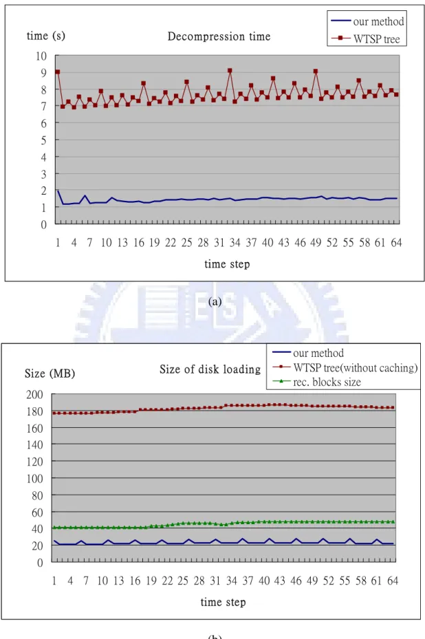
5.3 (a) The comparison of decompression time. We select a set of blocks of size 40 to 50 MB to be rendered. The decompression time for our algorithm and WTSP tree method is displayed in the figure. (b) The corresponding size of disk loading……….26
5.4 The rendering result image with tree difference scalar factors.……….….29
5.5 The temporal LOD selection. The green rectangular is the bounding box of temporal ROI. The blocks that are selected by the temporal ROI will be displayed in yellow bounding box, and only these selected blocks will be updated every time steps……….…….………….……….32
List of Tables
5.1 The data sets used in our testing………..21
5.2 The compression ratio with different number of I-frames in Jet_chi data set (total 122 time steps) ……….…..22 5.3 Compression of Jet_merg data set with our algorithm and WTSP tree…….…..23
5.4 The rendering speed with three different LOD selections at the first time step of the Jet_merg data set………..…..27 5.5 The playback speed of difference spatial LOD selections and temporal LOD
Chapter 1
Introduction
As computer storage and scanning precision rapidly increases, scientific measurements and simulations can generate large time-varying data set that have hundreds or thousands of time steps, and each time step may contain billions of voxels. Although direct volume rendering with 3D hardware texture mapping [Cabral et al. 1994; Westermann and Ertl 1998] can perform efficient rendering, the limited size of the texture memory makes it difficult to maintain an interactive frame rate when large data sets have to be rendered. When the data size of an individual time step does not fit into the available texture memory, a decomposition into blocks has to be applied to the data set. In this case, the texture memory swap-in and swap-out required for the entire volume reduce the rendering performances substantially. To overcome this problem, several multi-resolution schemes for static [LaMar et al. 1999; Weiler et al. 2000; Boada et al. 2001] or time-varying data [Shen et al. 1999] were proposed. These methods construct a multi-resolution hierarchy that represents different resolutions for different regions. They can adapt the data resolution to render the interesting or important regions with high accuracy, while other regions are rendered with lower accuracy. To further reduce the storage and data transmission bandwidth, some wavelet compression schemes were proposed [Guthe et al. 2002; Wang and Shen 2004]. These methods recursively apply wavelet transform to compress the data and in the end construct a multi-resolution hierarchical wavelet representation.
For time-varying data sets, user may not only want to navigate a specific time step with certain spatial or temporal level-of-detail, but also want to directly observe the temporal variations in the data. However, the current hierarchical wavelet compression schemes such as the wavelet-based time-space partitioning (WTSP) tree
using hierarchical wavelet transform, the reconstruction of the data requires a hierarchical decompression process. It will cause many additional disk loading and reconstruction overhead. In order to reduce reconstruction cost as much as possible, we can utilize temporal coherence and apply motion-compensation-based prediction in adjacent time steps. In this way, the reconstruction will not have hierarchical dependency. Once the corresponding data in the previous time step has existed in memory, we can directly reconstruct the data of the current time step.
Our algorithm constructs a system that is similar to a basic video coding structure: Each time step of the data set is classified as either an intra-coded frame (I-frame) or a predictive frame (P-frame). For an I-frame time step, we apply hierarchical wavelet transform to construct a multi-resolution hierarchical wavelet representation. The high-pass filtered coefficients are then encoded and stored in the disk. For a P-frame time step, we also use the hierarchical wavelet transform to construct a multi-resolution hierarchical representation. Then, we apply motion-compensation-based prediction to the low-pass filtered data. The resulting difference data and motion vectors are encoded and stored.
During rendering, the data is decompressed on-the-fly and rendered using hardware 3D texture mapping. The system allows the user to select a spatial region-of-interest (ROI) to adjust the spatial level-of-detail selection, and the selection of a temporal ROI to choose only a sub-region for frequent update during playback. With a suitable control of both ROIs, our system can reach an interactive playback frame rate. This allows the user to observe the dynamic properties of large time-varying data sets. We also propose caching and pre-loading mechanisms. Caching is applied in I-frame to help reusing previously reconstructed data blocks when the level of detail (LOD) selection is changed. Pre-loading is applied in P-frame to distribute the workload of each frame more evenly.
The remainder of this thesis is structured as follows: We first review related work in Chapter 2. Then, we describe the pre-processing compression scheme in Chapter 3. In Chapter 4, we describe the run-time decompression and rending of our system. Results are discussed in Chapter 5 and the conclusion is given in Chapter 6 with some ideas for future work.
Chapter 2
Related work
In this chapter, we give a brief overview of related work in the area of texture-based volume rendering, multi-resolution rendering, time-varying data compression scheme, and time-varying data hierarchical representation.
2.1 Texture-based Volume Rendering
The shear-warp factorization proposed by Lacroute and Levoy [Lacroute and Levoy 1994] is the most efficient software-based technique for direct volume rendering. They proposed the basic idea of using object-aligned textured slices to substitute trilinear by bilinear interpolation. This technique can be adapted to exploit 2D-texture hardware and achieve an interactive frame rate [Rezk-Salama et al. 2000]. The usage of hardware 3D texture mapping algorithm[Cabral et al. 1994; Westermann and Ertl 1998] allows for more flexibility and can provide a higher image quality. There are several advanced shading techniques proposed in recent visualization algorithms, such as lighting [Meißner et al. 1999], shadows [Behrens and Ratering 1998], high quality post-classification using a pre-integration technique [Engel et al. 2001], and gradient magnitude modulation[Van Gelder 1996].
2.2 Multi-resolution Rendering
The idea of multi-resolution volume rendering algorithms is to provide a spatial hierarchy to adapt the data resolution to render the interesting or important regions with higher accuracy, while other regions are rendered with lowerer accuracy. LaMar et al. [LaMar et al 1999] describe an octree-based multi-resolution approach for interactive volume rendering. They filter the volume to create levels-of-detail in an
3D texture mapping. A similar technique was proposed by Boada et al [Boada et al. 2001]. Their hierarchical representation benefits nearly homogeneous regions and regions of lower interest. Weiler et al. [Weiler et al. 2000] address the avoidance of discontinuity artifacts between different levels of detail. Their approach allows consistent interpolation between levels. These multi-resolution techniques can handle volume data sets that do not fit completely into the texture memory of the graphics hardware. However, the data must still fit into the main memory. Guthe et al. [Guthe et al. 2002] improved on this by using wavelet representation. They recursively apply wavelet transform to compress the data and construct a multi-resolution hierarchical wavelet representation. Their approach is able to render walkthroughs of large data sets in real time on a conventional PC.
Multi-resolution volume rendering provide a data hierarchy that supports level-of-detail (LOD). There are several types of criteria for the LOD selection. These LOD selection methods can be classified into four types. We give a brief overview to these LOD selection methods.
1. View-dependent criterion: This is a general criterion that takes the view- dependent factors into account. According to the position of viewer, it will let the regions that are closer to the viewer or the regions with larger projected screen area have higher resolution [LaMar et al. 1999; Guthe et al. 2002].
2. Region-of-interest: This criterion depends on the user-specified region- of-interest (ROI) to decide LOD selection [Pinskiy et al. 2001; Plate et al. 2002]. Usually there is a 3D bounding box to represent the ROI. User can change the size and the position of the bounding box. It will let the regions inside the ROI bounding box have higher resolution.
3. Data error metric: The data error metric calculates the error (usually the mean squared error) between the low resolution data block and the corresponding original volume data. Then, the LOD selection is decided by letting each subvolume satisfy the user-specified error tolerance [Shen et al.
1999; Wang and Shen 2004].
4. Image-based quality metric: The image-based quality metric evaluates the contribution of multi-resolution data blocks to the final image. Then, the LOD selection algorithm tries to choose a set of blocks that generate images of best visual quality [Ljung et al. 2004; Wang and Shen 2006; Wang et al. 2007].
2.3 Time-varying Data Compression Scheme
Guche and StraBer [Guthe and Straßer 2001] introduced an algorithm that uses the 3D wavelet transform to encode each individual volume, and then applies a motion-compensation-based prediction in adjacent time steps. Their algorithm is capable of decompressing and visualizing animated volume data at interactive frame rates. Sohn et al. [Sohn et al. 2002] proposed a volumetric video system that borrows the idea of MPEG compression to efficiently exploit spatial and temporal coherence. They encoded only the significant data that contribute to the iso-surface and volumetric feature to achieve high compression ratio with fast reconstruction. While the above two methods can perform efficient data compression and rendering, they are not designed for handling large time-varying data set that the size of an individual time step is larger than the texture memory, or is even larger than the main memory.
The compression scheme of our algorithm is similar to the method of [Guthe and Straßer 2001]. Their algorithm focuses on compressing the data as small as possible with fast reconstruction, using a lossy compression scheme where the rendering quality is decided during pre-processing and can not be changed later. Our algorithm addresses the combination of multi-resolution representation and such compression scheme. Even with a lossless compression of lower compression ratio, our system could achieve interactive playback of large time-varying data set by adjusting the LOD selection. If necessary, the rendering quality also can be enhanced by sacrificing the interactivity in the run-time.
2.4 Time-varying Data Hierarchical Representation
Linsen et al. [Linsen et al. 2002] proposed a four-dimensional multi-resolution approach for time-varying volume data. Their scheme treats temporal and spatial dimensions equally in a single hierarchical framework. The hierarchical data organization is based on 4
2 subdivision. The 4
2-subdivision scheme only doubles the overall number of grid points in each subdivision step. This fact leads to fine granularity and high adaptivity. Shen et al. [Shen et al. 1999] proposed time space partitioning (TSP) tree that captures both the spatial and temporal coherence of the underlying data. It allows the user to request spatial and temporal data resolutions independently with separate error tolerances. Ellsworth et al. [Ellsworth et al. 2002] later followed up the work and provided a hardware volume rendering using a TSP tee. They also proposed color-based error metrics that improve the selection of data blocks to be loaded into texture memory. Wang and Shen further utilized wavelet transform to propose wavelet-based time-space partitioning (WTSP) tree method [Wang and Shen 2004]. They first build a wavelet tree hierarchical representation [Guthe et al. 2002] for each individual time step. Then for the high-pass filtered coefficients from the corresponding spatial node along the time axis, they apply 1D wavelet transform to form a binary time tree. Although WTSP tree method supports flexible spatio-temporal multi-resolution data browsing, their hierarchical 1D wavelet compression of the spatial node along the time axis is not suitable for interactive playback.
Chapter 3
Compression Scheme
In this chapter, we describe our compression scheme. The input data is a time-varying volume data set, V = {V1, V2, ….., VT} with T time steps. In order to support
multi-resolution volume rendering, we first construct a multi-resolution data hierarchy for each time step. Then we apply our compression scheme on these hierarchy data. Each time step is classified as either an intra-coded frame (I-frame) or a predictive frame (P-frame). The compression of an I-frame is independent of the other frames, while compression of a P-frame is dependent on its previous frame.
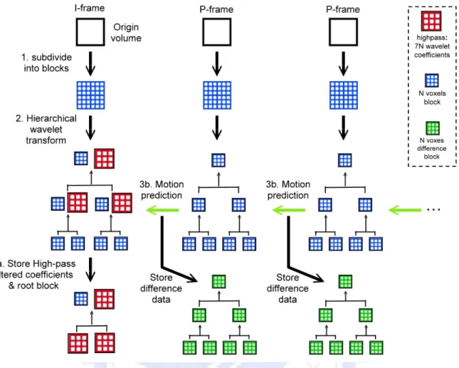
We illustrate the whole compression process as Figure 3.1. The steps of the compression scheme are as follows:
1. We subdivide the original volume of an individual time step into a sequence of blocks.
2. Then we recursively apply 3D wavelet transform to these blocks and construct a hierarchical wavelet representation.
3. (a). If this volume is an I-frame, we store the high-pass filtered coefficients and the low-pass filtered root block. The high-pass filtered coefficients are encoded before storing.
(b). If this volume is a P-frame, we apply motion-compensation-based prediction to each of its nodes from its corresponding spatial node in the previous frame. The resulting difference data and motion vectors are encoded and stored.
Figure 3.1: The compression process. Step 1 is to subdivide the original volume into a sequence of blocks. Step 2 is to apply 3D wavelet transform to these blocks and construct a hierarchical wavelet representation. In step 3, if this volume is an I-frame, the high-pass filtered coefficients are encoded. Then we store the encoded high-pass coefficients and the root data block. If this volume is a P-frame, we apply motion-compensation-based prediction from its corresponding spatial node in the previous frame. The resulting difference data and motion vectors are encoded and stored.
In the following section we will describe how we compress I-frame data and P-frame data in detail.
3.1 I-frame compression
We compress I-frame data using the wavelet-tree method [Guthe et al. 2002]. First, we divide the volume data of this frame into a sequence of blocks. Assuming
that the block size N is nx×ny×nz
N
, where , , and are all integers and
are all powers of 2. Then we apply 3D wavelet transform to each block. This will produce low-pass filtered coefficients and high-pass filtered coefficients. The low-pass filtered coefficients from eight adjacent blocks are collected and grouped into a new block of voxels (see Figure 3.2). Then we can apply this 3D wavelet transform and low-pass coefficients grouping process recursively until only a single block is left. This procedure produces an octree: Each node of the octree is a data block of voxels and contains a set of high frequency coefficients that allow for the reconstruction of the child nodes from the current node. The resolution of a child node is twice as high (in each dimension) as that of a parent node. We only keep the root low-pass filtered block and all the high-pass filtered data (see Figure 3.3). The other data blocks can be reconstructed by applying top-down inverse-wavelet transform recursively.
x n ny nz 8 / 8 / N 7N N
To reduce the size of the coefficients to be stored in the octree, the high-pass filtered coefficients resulting from the wavelet transform will be compared against a pre-defined threshold. The high-pass filtered coefficients are mapped to zero if they are smaller than the threshold. In our implementation, we set the threshold to zero, leading to a lossless compression. The high-pass filtered coefficients are then encoded using run-length encoding combined with a fixed Huffman encoder [Guthe et al. 2002]. The coefficients are first mapped to positive values: Positive coefficients are mapped to odd values (c→ c×2−1
n
) while negative coefficients are mapped to even values ( ). The encoding model is defined as follows: A run of zero coefficients is marked by a leading 0 bit. The following bits store the number of
Huffman code table. ) 2 (− × → c c
consecutive zeros. This results in 1 to
zero
n
zeros encoded in
bits and a leading 1 bit, with
zero n 2 nzero +1 pos n bits. Any
other coefficient is stored by using being the
minimum number of bits needed to represent the coefficient using a pre-defined
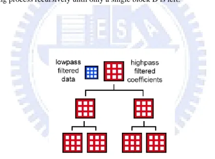
Figure 3.2: Construction of the wavelet tree. We apply 3D wavelet transform to each block, for example, block A and B in the figure. The low-pass filtered coefficients from eight adjacent blocks are collected and grouped into a new block C. Then we can apply this 3D wavelet transform and low-pass coefficients grouping process recursively until only a single block D is left.
Figure 3.3: The compressed wavelet tree of an I-frame. We only keep the root low-pass filtered block and all the high-pass filtered data.
3.2 P-frame compression
First we construct the octree hierarchy using the same method as I-frame, but we only keep the low-pass data of each level of the octree. Then for each node of the octree, we apply motion-compensation-based prediction from its corresponding
spatial node in the previous frame (see Figure 3.4). The steps of the motion-compensation-based prediction algorithm are as follows:
1. We further subdivide a node (a block with N voxels) into micro-blocks. A micro-block is a unit size for applying motion-compensation-based prediction.
The size of micro-block is lx×ly×lz. In our implementation, value of 4 or 8 is a suitable choice.
2. (a). For each micro-block, a best match, i.e. minimum mean squared error, in the corresponding spatial node of previous frame is computed by searching for this minimum. The displacement of this micro-block to the best match is called a motion vector (see Figure 3.5). We store the motion vector and the differences between a micro-block and its best match.
(b). Sometimes, a good match cannot be found – the prediction error exceeds a certain acceptable level. In this case each voxel of the micro-block is predicted from its neighboring voxels. If the result of this neighboring voxel prediction has smaller mean squared error, we store the predicted differences of each voxel.
3. Again, the differences data of all micro-blocks will be compared against a pre-defined threshold. The differences are mapped to zero if they are smaller than the threshold. We also set this threshold to zero in our implementation. The differences are then encoded using run-length encoding combined with a fixed Huffman encoder.
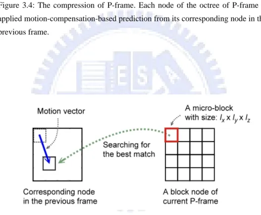
Figure 3.4: The compression of P-frame. Each node of the octree of P-frame is applied motion-compensation-based prediction from its corresponding node in the previous frame.
Figure 3.5: Motion-compensation-based prediction for a block node. For each micro-block of current processing P-frame, we search the best match in the corresponding node in the previous frame. The resulting motion vectors and difference data is then encoded and stored.
Chapter 4
Rendering
In the pre-processing compression stage, the given time-varying volume data set has been transformed into a sequence of compressed data. In this section, we will describe the run-time decompression and rending of our system.
The system starts from a LOD selection that chooses a list of blocks to be rendered. We introduce our LOD selection method in Section 4.1. In Section 4.2, we describe the decompression and reconstruction of the data blocks in the selected blocks at run-time. In Section 4.3, we render the volume data using hardware texture mapping. In Section 4.4, we propose a caching and pre-loading mechanism that helps our system achieve better performance.
4.1 Level of Detail Selection
In our system, the spatial LOD selection is decided by considering region of interest (ROI) and some view-dependent parameters. The ROI is specified by a 3D bounding box. Users can change the size of the bounding box and arbitrarily move the bounding box to adjust the LOD selection. This method provides an intuitive and flexible way to specify LOD selection.
In order to reduce the total size of updated blocks along time axis and achieve an interactive playback, we provide the user the temporal ROI to choose only a sub-region for per-frame update. This temporal ROI is another 3D bounding box that can be controlled in the spatial space by the user. When the temporal ROI is enabled, the system first decides the spatial LOD selection by the spatial ROI and view-dependent parameters, and then only the data blocks that is selected by the temporal ROI will be updated at every time step. Blocks that are outside the temporal
4.1.1 Spatial LOD selection
The spatial LOD selection will choose a list of blocks from the octree hierarchy for rendering. In order to avoid texture swapping-in and swapping-out in a single rendering pass, the total texture size of selected blocks should not exceed the texture memory of the graphics hardware. Usually the user may want to set a maximum amount of blocks size MLOD for this spatial LOD selection. We provide a scalar
, and the maximum amount of selected blocks size MLOD will be: factor φS
TEX S LOD M
M =φ ⋅
where MTEX is the maximum available texture m mory of the graphics hardware, and the value of
e
S
φ is within 0.0 to 1.0. Higher value of φS will have better rendering quality, while lower value of φS will make the rendering or playback faster.
Users can change the value of φS in the run-time to trade the rendering quality for
The spatial LOD selection algorithm i achieved by traversing the octree with a priority queue. Each node i of the octree hierarchy will have a priority value
distance to the viewer position: rendering or playback speed.
s
. The priority value is given by considering the ROI bounding box and the ) (i PLOD ) ( ) ( ) (i C1 P i C2 P i
PLOD = ⋅ ROI + ⋅ VIEW
1
C and C2 are weighting coefficients. We now define PROI(i) and PVIEW(i)
as follow: where
1. : This function will let the regions which are inside the ROI bounding box have the highest priority value, and let the regions which are outside the ROI bounding box get lower and lower priority value while
center is inside the ROI bounding box, its priority value will be . For other nodes that are outside the ROI bounding box, we set )
(i
PROI
set to 1
the distance to the ROI bounding box is increased. For the node whose )
(i
)) ( 1 /( 1 ) (i D i
PROI = + ROI where DROI(i) is the distance from the center of node i to the ROI bounding box.
2. P (i): Since the node that is closer to the viewer usually contributes more to the final image. This function lets the nodes that are closer to the viewer have higher priority value. We set PVIEW(i) 1/(1+DVIEWER(i))
VIEW
= ,
we create an em where )DVIEWER(i
In the beginning of the algorithm,
is the distance from the node
pty priority queue and insert the root node
i to the viewer.
r of the octree hierarchy
ly fetch
eight child nodes into the queue. If a leaf the priority queue and put
maximum
queue into the rendering queue. All the nodes
e steps. In order to achieve in
e can use the temporal ROI every time step. The blocks th
into the que
it into another queue for
layback, we
ue with priority . Then we e
from
Th iority q
qu priority
in the rendering queue will be used for
tim teractive p provide another temporal ROI
bounding box to specify which blocks will be pdated at at are inside the temporal ROI bounding box
temporal ROI bounding box to )
(r
PLOD
storing nodes to be rendered. ueue and
successiv the node with the highest priority from the queue, and insert its node is reached, we remove this leaf node
is procedure stops when the total blocks size of the pr rendering eue reaches the size MLOD. Then we put all the nodes in the
rendering.
4.1.2 Temporal Region of Interest
After the spatial LOD selection, we have chosen a set of blocks that provide a suitable approximation to the original volume in a single time step. But even with this smaller approximation data set, there is still too much data for updating all blocks in every
bounding box. From the blocks that have been chosen by the spatial LOD selection algorithm, w
u
will be updated at every time step, while the others will be updated only at every I-frame (see Figure 4.1). The user can change the
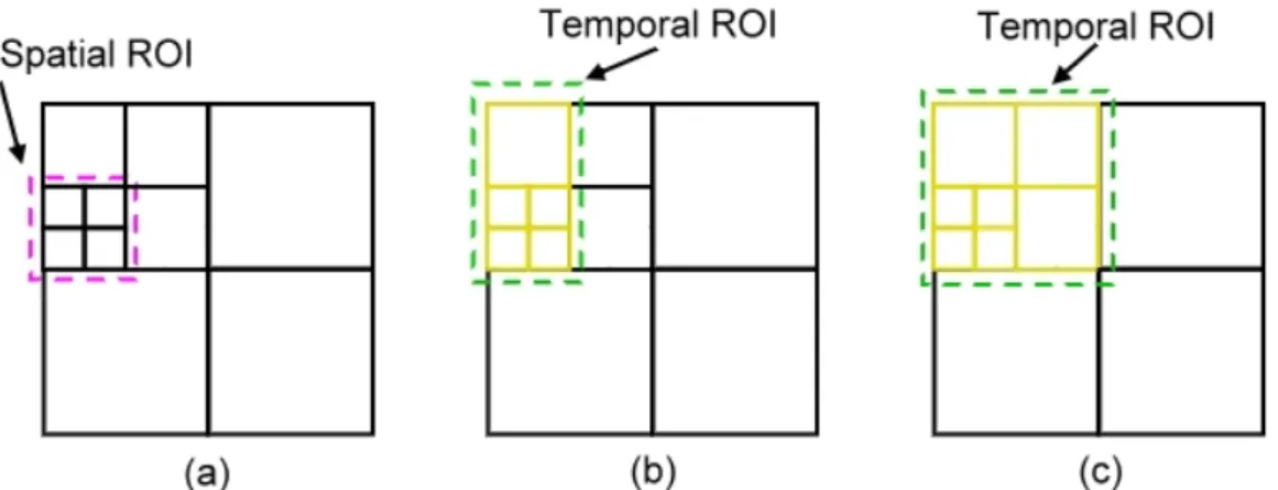
Figure 4.1: The temporal ROI. The current spatial LOD selection is decided by the spatial s in (a). When the temporal ROI is enable as (b) and (c), only the blocks that is selected by temporal ROI (denoted as yellow blocks) will be updated at every time step during playback. In (b), there are only 5 blocks that are selected by the temporal ROI. In (c), there are 7 blocks that are selected by the temporal ROI.
4.2 Run-Time Decompression
Once we have decided the spatial LOD selection in I-frame, we need to d
s o
w nd apply inverse 3D wavelet
ansform to obtain the data of its eight child blocks. We recursively take these ecompressed blocks and their corresponding high-pass filtered coefficients to
n traversal meets a block node that is selected by the spatial LOD selection, we stop the traversal of this node.
ROI a
ecompress these blocks data from disk. For an I-frame, the decompression procedure tarts at the root node of the octree hierarchy. We load the low-pass filtered block data f the root node and its corresponding high-pass filtered coefficients from disk. Then
e decode these high-pass filtered coefficients a tr
d
reconstruct their child blocks. When the reconstructio
For a P-frame, its spatial LOD selection is decided by the previous I-frame. Since each block of a P-frame is predicted from its corresponding block in the previous frame, once all the blocks of its previous frame are reconstructed, we can decode the difference data from disk and recover the blocks data of P-frame.
4.3 Rendering of Blocks
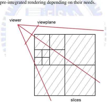
To render these selected blocks, we use texture-based volume rendering. We draw all blocks in back-to-front order. The order can be established by enforcing a back-to-front traversal order of the octree. For each block, a 3D texture is created and loaded into the texture memory. We place view-aligned slices into the block (see Figure 4.2) and render these slices in back-to-front order. Alpha blending delivers the
he pixels on the screen.
To obtain a higher rendering quality, we provide pre-integrated volume rendering volume integrals along viewing rays for all t
[Engel et al 2001]. The pre-integrated volume rendering requires more texture fetching to render the slices, hence it will consume more time for rendering. Users can turn on or off pre-integrated rendering depending on their needs.
Figure 4.2: Rendering with view-aligned slices
4.4 Caching and Pre-Loading
mechanisms. Caching usly reconstructed data blocks when the LOD selection is ch pplied in P-frame to istribute the workload of each frame more evenly. We will allocate a pre-defined amount of additional main memory and texture memory for caching and pre-loading.
ach cached block a deleting priority . If we run short of memory, we . We define the deleting priority as:
is applied in I-frame to help reusing previo anged. Pre-loading is a d
4.4.1 Caching
In I-frame, user may often change the spatial ROI bounding box to adjust spatial LOD selection. Some of the data blocks that are currently useless may be useful again in the future time. To save the time for loading and reconstructing these data blocks, we cache all the decompressed data blocks in main memory during I-frame. We give
e i
delete the data blocks that have the highest
) (i PDEL (i PDEL ) ) (i
PDEL for each block i
) ( ) ( ) ( ) (i W1L i W2C i W3F i PDEL = + +
where W1, W2, and W are weighting coefficients. We now define 3 L(i), )C(i , and )
(i
F as follow:
1. L(i): This function considers the likelihood of a block node being visited. A block node will be visited for decomp
it is closer to the root of the octree hierarchy. Thus, we define L(i) of block node i
ressing child nodes more often when
as their depth in the octree. The root node is at depth zero.
2. : This function is defined using a least recently used (LRU) scheduling e. We give each decompressed block in memory a counter that
et
ter of each block is updated as: )
(i C
schem C(i)
is initially s to zero. Every time when spatial LOD selection is changed, the coun C(i) ⎩ ⎨ ⎧ = + = otherwise. , 0 ) ( used. not is block when , 1 ) ( ) ( i C i i C i C
It means that the least recently used blocks will get higher deleting priority.
nter for each block of tree hierarchy. is initially set to zero. Ev e when a block decompressed into m value of is increased by 1. can be calculated as:
3. F(i): This function is an auto-adapting term for the blocks that are swapped in and out frequently. If we find a data block is swapped in and out frequently, it is better to cache this block for performance consideration. To realize this function, we define a loading cou
th
i is loaded from emory, the
if S(i) S , F(i) 1 (S(i) S ) ) (i S ery tim THRE e oc S(i) disk and
Then the value of
) (i S ) (i F THRE =− × − > , else, F(i)=0
where STHRE is a pre-defined threshold value. Thus, if a block is swapped in and out too frequently, i.e. S(i)>STHRE, we will decrease its deleting priority.
e have explained our caching mechanism for main memory. The cach e
onsider the effect of visitin eed to vis locks in texture memory for deco res
) ) ( ) ( ) (i W2C i W3F i PDEL W ing of texture
m mory is the same as the one of main memory, except that this time we do not c g likelihood , since we do not n it these b mp child nodes. The deleting priority
for each block of texture mem ry is defined as: ) (i L sing o (i PDEL i + = e step, while o
workload of P-fram en encountering an
4.4.2 Pre-loading
When temporal LOD is enabled, data blocks that are selected by temporal ROI bounding box will be updated at every tim thers will be updated only at every I-frame. It means that the workload of I-frame is usually much larger than the
I-frame. To distribute the workload more evenly, at P-frame we can pre-load the data blocks of the next I-frame in advance. This will make the playback smoother.
Chapter 5
Result
In this chapter, we discuss the experimental result obtained with an implementation of our algorithm. The algorithm was implemented in C++ and OpenGL. All benchmarks were performed on a 2.4GHz Intel core 2 processor with 2GB main memory , and an nVidia GeForce 8800 GTX graphics card with 768MB video memory.
5.1 Example Data Sets
The time-varying data set used in our testing is Turbulent Combustion Simulation data set from the Institute of Ultra-Scale Visualization (IUSV). This data set is made available by Dr. Jacqueline Chen at the Sandia National Laboratory through SciDAC IUSV. The original data set consists of five floating variables. There are
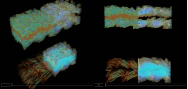
voxels, and a total of 122 time steps. For simplicity reason, we convert the floating variables into 16-bit integers. We take one of the variables named “chi” as our test data set – Jet_chi (see Table 5.1). Another data set Jet_merg (see Figure 5.1) is obtained by merging four variables to form a larger data set. It has
voxels in each time step, and a total of 64 time steps. The data size of each time step is 949 MB, and the total size of 64 time steps is 59.3 GB.
120 720 480× × 360 1440 960× ×
Table 5.1: The data sets used in our testing. Data set Resolution Time steps Size of each
time step
Total size
Jet_chi 480×720×120 122 79.1 MB 9.42 GB Jet_merg 960×1440×360 64 949 MB 59.3 GB
Figure 5.1: The Jet_merg data set.
5.2 Preprocessing Result
In Jet_chi data set, we chose the block size to be 128×256×32 and each block is of size 2MB. This leads to a 3-level hierarchy octree with 73 nodes. In Jet_merg data set, we chose the block size to be 64×128×32, and each block is of size 0.5 MB. This leads to a 5-level hierarchy octree with 4681 nodes. We use Haar wavelet transform with lifting scheme in all our tests for simplicity and efficiency reasons. We first test the compression ratio with different number of I-frames in Jet_chi data set. The result is displayed in Table 5.2. Lossless compression scheme is used. It shows that our P-frame compression is slightly better than the conventional wavelet-tree (I-frame) method.
Table 5.2: The compression ratio with different number of I-frames in Jet_chi data set (total 122 time steps).
No. of I-frame : No. of P-frame 13 : 109 25 : 97 61 : 61 122 : 0 Total size 1.85 GB 1.87 GB 1.92 GB 2.02 GB Compression ratio 5.091:1 5.037:1 4.906:1 4.663:1
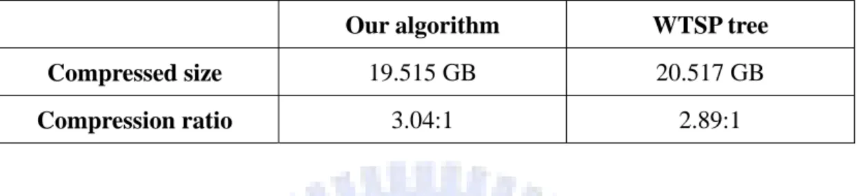
with our algorithm. We set all compression parameters the same to compress the Jet_merg data set with WTSP tree method and our algorithm.The compression result is displayed in Table 5.3. Our algorithm can achieve higher compression ratio than WTSP tree method.
Table 5.3: Compression of Jet_merg data set with our algorithm and WTSP tree. Our algorithm WTSP tree Compressed size 19.515 GB 20.517 GB
Compression ratio 3.04:1 2.89:1
From the result of Table 5.2, we can see that the P-frame compression does not enhance compression ratio as much as in video compression. It is because the tested scientific data do not behave like rigid body motion, and the variation between two consecutive frames is much more than in general video. Thus, the temporal coherence is much harder to catch and the motion-compensation-based prediction is not as effective as in general video system.
5.3 Run-Time Rendering Result
During rendering, the selected blocks will be decompressed on-the-fly and then uploaded to texture memory for texture mapping. In all the following tests, we set the maximum available texture memory MLOD as 512MB for spatial LOD selection.
5.3.1 Decompression Time
Here we test our decompression efficiency with Jet_merg data set and compare it to the WTSP tree method. We test the decompression time and disk loading bandwidth in our system and in the WTSP tree method. In Figure 5.2, the LOD selection chooses out a set of blocks of size 20 to 30 MB. In Figure 5.2(a), we compare the
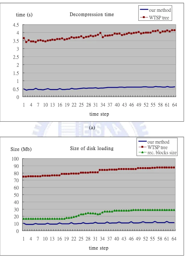
display the corresponding disk loading bandwidth. In Figure 5.3, we display another test result under different spatial LOD selections. The LOD selection chooses out a set of blocks of size about 40 to 50 MB. The decompression time includes disk I/O to fetch compressed data, decoding the compressed bit streams, and reconstruction of data blocks. The comparison is tested under the same situation. The rendering results are identical in both methods. We assume that we don’t have additional memory space to cache intermediate nodes in the binary time tree of WTSP tree method. We also disable the caching and pre-loading mechanism in our system.
In the comparison result we can see that the decompression time of our system is obviously less than that of the WTSP tree method. It is because of the large additional overhead to traverse the binary time tree in the WTSP tree method. This problem will get worse when the number of time steps is increased. In our algorithm, even without additional memory space, we can decompress the data blocks efficiently, and the performance is independent of the number of time steps. In Figure 5.2, the playback frame rate of WTSP tree method is 0.264 fps when there are only 64 time steps. Our method can reach a playback frame rate of 1.834 fps under the same situation.
Decompression time 0 0.5 1 1.5 2 2.5 3 3.5 4 4.5 1 4 7 10 13 16 19 22 25 28 31 34 37 40 43 46 49 52 55 58 61 64 time step
time (s) our method WTSP tree
(a)
Size of disk loading
0 10 20 30 40 50 60 70 80 90 100 1 4 7 10 13 16 19 22 25 28 31 34 37 40 43 46 49 52 55 58 61 64 time step Size (Mb) our method WTSP tree rec. blocks size
(b)
Figure 5.2: (a) The comparison of decompression time. We select a set of blocks of size 20 to 30 MB to be rendered. The decompression time for our algorithm and WTSP tree method is displayed in the figure. (b) The corresponding size of disk loading.
Decompression time 0 1 2 3 4 5 6 7 8 9 10 1 4 7 10 13 16 19 22 25 28 31 34 37 40 43 46 49 52 55 58 61 64 time step time (s) our method WTSP tree (a)
Size of disk loading
0 20 40 60 80 100 120 140 160 180 200 1 4 7 10 13 16 19 22 25 28 31 34 37 40 43 46 49 52 55 58 61 64 time step Size (MB) our method WTSP tree(without caching) rec. blocks size
(b)
Figure 5.3: (a) The comparison of decompression time. We select a set of blocks of size 40 to 50 MB to be rendered. The decompression time for our algorithm and WTSP tree method is displayed in the figure. (b) The corresponding size of disk loading.
5.3.2 LOD and Rendering Speed
In Table 5.4, we list the rendering speed with three different scalar factor φS at
5.4.
the first time step of the Jet_merg data set. We also show the result images in Figure
able 5.4: The rendering speed with three different LOD selections at the first time step of the T
Jet_merg data set
= 0.0924 φS
= 0.2442 φS = 0.033
S
φ
No. of total blocks 246 92 29 No. of non-uniform blocks 228 88 25 Size of non-uniform blocks 114 MB 44 MB 12.5 MB
Rendering frame rate 19.81 29.89 31.14 Rendering frame rate (pre-integrated) 18.18 19.15 19.97
(a)
(b)
(d) (e)
(f)
Figure 5.4: The rendering result image with tree difference scalar factors. (a): The rendering result with φS = 0.033. Its corresponding LOD selection is showed in (d). The white string lines stand for the bounding box of each block. (b): φS = 0.924. Its corresponding LOD
selection is showed in (e). (c): φS = 0.2442. Its corresponding LOD selection is showed in (f).
From the result, we show that we can lower down the value of φS in the
n-time to trade rendering quality for rendering speed. User can roughly browse the data
ru
set and find out suitable camera parameters quickly with smaller φS in the beginning, and then increase φS to reveal more detail.
the selected blocks of temporal ROI with yellow bounding boxes in Figure 5.5. The size of the temporal ROI is 18 of the whole volume size. Decreasing the value of
S
φ and using temporal ROI helps to enhance the playback frame rate. Here we
Table 5.5: The playback speed of difference spatial LOD selections and temporal LOD selections. demonstrate that with the flexible spatial and temporal LOD selection mechanism, user can easily achieve an interactive playback.
S
φ = 0.2442 φS = 0.2442
(With Temporal ROI)
S
φ = 0.0924 φS = 0.0924
(With Temporal ROI)
S
φ = 0.033 φS = 0.033
(With Temporal ROI)
No. of non-uniform 230 146 84 45 21 10 blocks Size of non-uniform blocks 115 MB 73 MB 42 MB 22.5 MB 10.5 MB 5 MB Playback frame rate 0.272 0.425 1.151 1.841 4.13 7.81
(a). φS = 0.2442. Temporal ROI elected blocks size: 73 MB. Playback frame rate: 0.425.
(b). φS = 0.0924. Temporal ROI elected blocks size: 22.5 MB. Playback frame rate: 1.84.
Figure T x of temporal ROI. The blocks that are selected by the temporal ROI will be displayed in yellow
5.5: he temporal LOD selection. The green rectangular is the bounding bo
Chapter 6
Summary and Future Work
6.1 Summary
We have introduced a new framework that combines the multi-resolution hierarchical representation with video-based compression to manage and render large scale time-varying data. We demonstrate how this new structure can perform more efficient reconstruction in time axis with respect to the WTSP tree method. We also provide flexible user-assisted mechanism to easily achieve interactive playback in the run-time. Our main contribution is to provide the user the ability to observe the dynamic change in interactive frame rate. We believe that the ability of interactive playback can help the users to reveal more information in large time-varying volume data, which is not available in the previous multi-resolution representation.
6.2 Future work
We currently use the temporal ROI to choose a sub-region for full update along time axis. We could calculate the temporal error of each block in the pre-processing stage. User can specify a temporal error tolerance. In the run-time, we can update only the blocks whose temporal errors are larger than the error tolerance.
Since we construct a new structure that combines the multi-resolution hierarchical representation with video-based compression, we could adapt the current advanced video compression techniques to improve the compression and decompression efficiency. Since the size of our approach for a large time-varying data set may still be too large to handle on a single PC, we could distribute the multi-resolution data into a parallel or multi-server network visualization system to achieve real-time rendering.
Bibliography
[Behrens and Ratering, 1998] Behrens, U., Ratering, R.: Adding shadows to a texture-based volume renderer. In: IEEE Symposium on Volume Visualization, IEEE, ACM SIGGRAPH, 39–46., 1998.
[Boada et al., 2001] Boada, I., Navazo, I., Scopigno, R.: Multiresolution volume visualization with a texture-based octree. In: The Visual Computer, 17(3), 185.197. Springer, 2001.
[Cabral et al., 1994] Cabral, B., Cam, N., Foran, J.: Accelerated Volume Rendering and Tomographic Reconstruction Using Texture Mapping Hardware. Symposium on Volume Visualization, 1994.
[Ellsworth et al., 2000] Ellsworth, D., Chiang, L. J., and Shen, H. W.: Accelerating Time-Varying Hardware Volume Rendering Using TSP Trees and Color-Based Error Metrics. In Proceedings of IEEE Symposium on Volume Visualization ’00, ACM Press, 119–129, 2000.
[Engel et al., 2001] Engel, K., Kraus, M., Ertl., T.: High-quality pre-integrated volume rendering using hardware-accelerated pixel shading. In Proc. of Eurographics/SIGGRAPH Workshop on Graphics Hardware, 2001.
[Guthe et al., 2002] Guthe, S., Wand, M., Gonser, J., and Straber, W.: Interactive Rendering of Large Volume Data Sets. In Proceedings of IEEE Visualization ’02, IEEE Computer Society Press, 53–60, 2002.
[Guthe and Straßer, 2001] Guthe, S., and Straßer, W.: Real-Time Decompression and Visualization of Animated Volume Data. In Proceedings of IEEE
Visualization'01, IEEE Computer Society Press, 349–356, 2001.
[Lacroute and Levoy, 1994] Lacroute, P., Levoy, M.: Fast volume rendering using a shear-warp factorization of the viewing transformation. In: Computer Graphics, 28 (Annual Conference Series), 451–458, 1994.
Hierarchical Representation of Time-Varying Volume Data with "4th-root-of-2" Subdivision and Quadrilinear B-Spline Wavelets. In Proceedings of Pacific Conference on Computer Graphics and Applications, 346, 2002.
[Ljung et al., 2004] Ljung, P., Lundstrom, C., Ynnerman, A., and Museth, K.: Transfer Function Based Adaptive Decompression for Volume Rendering of Large Medical Data Sets. In Proceedings of IEEE Symposium on Volume Visualization and Graphics ’04, 25-32, 2004.
[LaMar et al., 1999] LaMar, E.C., Hamann, B., Joy, K.I.: Multiresolution techniques for interactive texture-based volume visualization. In: IEEE Visualization'99, pages 355–362, 1999.
[Meißner et al., 1999] Meißner, M., Hoffmann, U. Straßer, W.: Enabling
Classification and Shading for 3D Texture Mapping Based Volume Rendering using OpenGL and Extensions. In: IEEE Visualization ’99, 207–214, 1999.
[Pinskiy et al., 2001] Pinskiy, D., Brugger, E., Childs, H., and Hamann, B.: An octree-based multiresolution approach supporting interactive rendering of very large volume data sets. In Proceedings of The International Conference on Imaging Science, Systems, and Technology ’01, 16-22, 2001.
[Plate et al., 2002] Plate, J., Tirtasana, M., Carmona, R., and Frohlich, B.:
Octreemizer: a hierarchical approach for interactive roaming through very large volumes. In Proceedings of IEEE symposium on Data Visualization, 2002.
[Rezk-Salama et al., 2000] Rezk-Salama, C., Engel, K., Bauer, M., Greiner, G., Ertl, T.: Interactive Volume Rendering on Standard PC Graphics Hardware using Multi-Textures and Multi-Stage Rasterization. In: Eurographics/SIGGRAPH Workshop on Graphics Hardware, 2000.
[Sohn et al., 2002] Sohn, B. S., Bajaj, C., and Siddavanahalli, V.: Feature Based Volumetric Video Compression for Interactive Playback. In Proceedings of IEEE Symposium on Volume Visualization ’02, ACM Press, 89–96, 2002.
[Shen et al., 1999] Shen, H. W., Chiang, L. J., and Ma, K. L.: A Fast Volume Rendering Algorithm for Time-Varying Fields Using a Time-Space Partitioning (TSP) Tree. In Proceedings of IEEE Visualization ’99, IEEE Computer Society
Press, 371–377, 1999.
[Van Gelder and Kim, 1996] Van Gelder, A., Kim, K.: Direct Volume Rendering with Shading via Three-Dimensional Textures. Symposium on Volume
Visualization, 23-30, 1996.
[Wang and Shen, 2004] Wang C., Shen H. W.: A Framework for Rendering Large Time-Varying Data Using Wavelet-Based Time-Space Partitioning (WTSP) Tree. Tech. Rep. OSU-CISRC-1/04-TR05, Department of Computer and Information Science, The Ohio State University, January 2004.
[Wang and Shen, 2006] Wang, C., and Shen H. W.: LOD Map - A Visual Interface for Navigating Multiresolution Volume Visualization. In IEEE Transactions on Visualization and Computer Graphics, 1029-1036, 2006.
[Wang et al., 2007] Wang, C., Garcia, A., and Shen H. W.: Interactive
Level-of-Detail Selection Using Image-Based Quality Metric for Large Volume Visualization. In IEEE Transactions on Visualization and Computer Graphics, 122-134, 2007.
[Weiler et al., 2000] Weiler, M., Westermann, R., Hansen, C. Zimmerman, K., Ertl, T.: Level-of-detail volume rendering via 3d textures. In: IEEE Volume
Visualization and Graphics Symposium, 2000.
[Westermann and Ertl, 1998] Westermann , R. and Ertl, T.: Efficiently Using Graphics Hardware in Volume Rendering Applications. In Proc. of SIGGRAPH, Comp. Graph. Conf. Series, 1998.