Who Are Reluctant to Realize Their Losses?
Pei-Gi Shu*Associate Professor,
Department of Business Administration, Fu-Jen Catholic University Yin-Hua Yeh
Professor
Department of International Trade and Finance, Fu-Jen Catholic University Shean-Bii Chiu
Professor
Department of Finance, National Taiwan University Hsuan-Chi Chen
Associate Professor
Department of Finance, Yuan-Ze University
Abstract
This paper investigates the disposition effect of individual investors from a data set of 53,680 accounts covering 10,883,473 transaction records. The results show that investors in Taiwan exhibit disposition effect to an extent more than the U.S. investors. The results of logistic regression and tobit regression show that aged female is more inclined to asymmetrically deal with their winners than losers. In contrast, the margin-purchase or short-selling investor is less to be the pawn of the disposition effect. We also explore the situations faced by investors and find that investors in the high-absolute-return quartiles are not disposed.
JEL classification: D14; D31
Keywords: the disposition effect, investor characteristics, self-control mechanism .
I. Introduction
The disposition effect is one implication extended from Kahneman and Tversky’s (1979) prospect theory and labeled by Shefrin and Statman (1985) illustrating that individual investors have the tendency to realize their winners too soon and hold losers too long. Under prospect theory, the value function of an investor is defined on gains and losses rather than on levels of wealth. The function is concave in the domain of gains and convex in the domain of losses. It is also steeper for losses than for gains, implying investors are generally risk-averse. An investor behaves to maximize the “S”-shaped value function.
Why an investor reacts differently to his investments that have declined in value and to the ones that have appreciated in value? Literature offers two threads of thinking: rational and irrational. Recognizing bounded rationality of investors, Thaler (1985) suggests that investors keep track of gains and losses in separate mental accounts, and to reexamine each account only intermittently when action relevant. Having observing losses an investor triggers his unpleasant feeling and is thus reluctant to recognize losses. Self-deception theory reinforces this argument since a loss is an indicator of low decision ability. The rational explanations include (1) expecting short-term mean reversion of stocks (Andreassen, 1988); (2) selling some of appreciated stocks on the purpose of diversification (Lakonishok and Smidt, 1986); (3) believing that the information of appreciated stocks has fully reflected on price while that of depreciated stocks has not yet been incorporated into price (Lakonishok and Smidt, 1986); and (4) avoidance of trading low-price stocks, which tend to be losers, under the consideration of high transaction costs of these stocks (Harris, 1988).
One pioneering empirical study is ascribed to Odean (1998) who obtains the trading records for 10,000 accounts from a large discount brokerage house and evidences the disposition effect for the U.S individual investors. He also finds that investors engage in tax-motivated selling in December, which decreases the discrepancy of investor’s inclination to realizing gains than losses.
In this study we investigate the behavior of individual investors from a data set obtained from a Taiwanese brokerage house, beginning from January 1998 and ending September 2001, of 53,680 accounts covering 10,883,473 transaction records. The data set is more abundant and more recent than the one used by Odean. Moreover, the case of Taiwan provides an opportunity for the further understanding of the disposition effect since the stock markets in Taiwan are mainly composed of individual investors who tend to be active investors with turnover ratio far exceeding their counterparts all over the world1. Moreover, the data set studied herein includes demographic statistics that allow us to contrast the effect of different investors with different characteristics.
The results show that investors in Taiwan exhibit disposition effect to an extent more than the U.S. investors. On average, the proportion of realizing gains is 2.5 times that of realizing losses. And the average excess returns on paper losses are lower than those on realized gains for the holding periods of 1-,3-,6-, 9-, and 12 months subsequent to the sales of a realized gain and subsequent to days on which sales of other stocks take place in portfolio of a paper loss.
Moreover, logistic regression as well as tobit regression are used to investigate the
1 The composition of investors in the Taiwanese equity market is quite different from that in the US
equity market. Individual investors comprise 90% of the market value in 1998 and 84% in 2001. These investors are quite active in trading. The turnover ratio of Taiwan equity market is 314% in 1998 and
characteristics that affect an investor’s inclination on realizing gains than losses. The results indicate that aged females, who tend to be nonprofessional investors with limited knowledge, are more inclined to asymmetrically deal with their winners than losers. In contrast, the margin-purchase or short-selling investors levering their position through margin are less to be pawns of the disposition effect.
We also explore the situations that affect an investor’s attitude to deal with his winners and losers by partitioning sample based on the quartiles of absolute return and stock price. PGR/PLR is less than 1 for the high-absolute-return quartiles, indicating that the investors trigger self-control mechanism in order to bound losses within tolerable limit and also forbear from realizing intermittent small gains. However, it is less clear why investors in low-absolute-return group are also less disposed. The rest of this paper is organized as follows. Section I is introduction. Section II describes the data set and Section III introduces methodology. Section IV reports the empirical findings. Section V concludes.
II. The Data
The data for this study are provided by a well-known securities brokerage house in Taiwan. From all accounts active beginning from January 1998 and ending September 2001, 53,680 customer accounts are randomly selected. The data are composed of three files: a customer file, a trade file, and a position file. The customer file includes branch identifier, account identifier, ID number, date of birth, latest date of trading, an electronic dummy that signifies if trading of account is executed through electronic system, and a margin dummy is assigned value 1 if it is margin-purchase or short-selling account. The trade file includes the records of all
trades made in the 53,680 accounts. This file has 1,088,473 records, each record is made up of trading date, trading type (cash trading, long or short margin trading, margin call), buy/sell identifier, branch identifier, the internal number for securities traded, the quantity traded, trading price, the principal amount, and the transaction taxes. The monthly position file is replicated from the updated information on November 9, 2001. The file contains date, branch identifier, account identifier, the internal security number, and quantity. Our sample is free from survivorship bias that might be in favor of more successful investors since there is no closed account throughout the sampling period.
Since our data set is left censored from January 1998, there will be securities that were purchased before then for which the purchase price is not available. And investors may also have accounts in other brokerage house that are not part of the data set. Even though the data set contains only part of each investor’s total portfolio, there is no special reason to doubt that the selection process will bias investor’s preference for realizing gains or losses.
The data set studied herein is more abundant and recent than the data used in previous studies. For example, a large retail broker provide 2,500 accounts for Schlarbaum et al. (1978) and others and 3,000 accounts for Badrinath and Lewllen (1991) and others in analyzing whether the ratio of stocks sold for a loss to those sold for a gain is affected by tax-motivated trading. In contrast, Odean (1998) obtains 10,000 accounts from a discounted brokerage house in investigating the disposition effect. Even though the disposition effect proposed by Odean (1998) is of interest and explored in this study, our data potentially contributes to literature for further understanding of investor’s behavior. First of all, the number of accounts used herein is 5.36 times of that used in Odean, the number of trading records is 66.79 times of
that in Odean. In other words our data is more representative to illustrate the behavior of individual investors than the ones used in previous studies. Moreover, given that on average Taiwanese investors are frequent traders, the imbalance between selling winners and selling losers accentuated in the disposition effect should be more pronounced if the results follow its dictum. Finally, our sampling period covers the eras of bullish as well as bearish markets and results in a conclusion sustainable to the change of market condition.
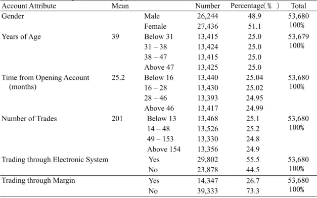
Table 1 summarizes the distribution of account attributes. The data show that the accounts of male (26,244, 48.9%) and those of female (27,436, 51.1%) are basically evenly distributed. The attributes of age, time from opening account to the yearend of 2001, and trading frequency are equally classified into quartiles. The median of investors’ age is 38, and 50% of investors are in the range of 31- to 47 years of age. The majority of investors have 1-3 years of experience to deal with the brokerage house. The distribution of trading frequency is highly skewed to right with the mean frequency of 201 times and the median of 48 times.
<< Insert Table 1 Here>>
III. Methodology
This study follows Odean (1998) to test whether investors sell their winners too soon and hold losers too long. Each day that a sale takes places, the selling price for each stock sold to its average purchase price between the latest two selling days are compared and determined whether that stock sold is recognized as a gain (realized gain) or a loss (realized loss). For those stocks in portfolio but not sold in that day, if
both its daily high and low are above (below) its average purchase price between the latest two selling days it is counted as a paper gain (loss); if its average price lies between the high and low, neither a gain or loss is counted. On days when no sales take place in an account, no gains or losses, realized or paper, are counted. Realized gains, paper gains, realized losses, and paper losses are simply the counts across all accounts over the sampling period beginning from January 1998 and ending September 2001.
In order to circumvent the impact of market conditions on the counts of selling winners versus losers2, Proportion of Gains Realized (PGR) and Proportion of Losses
Realized (PLR) are calculated as follow.
PGR =Realized Gains / (Realized Gains + Paper Gains) (1)
PLR =Realized Losses/ (Realized Losses + Paper Losses) (2)
The test of the disposition effect is a joint test that investors are disposed to dealing with gains and losses and the specification of reference point. The reference point refers to an investor’s perception of the true cost of his purchased stocks. However, it seems unlikely to vindicate the true reference point. Some possible choices of a reference point for stocks are the average purchase price, the highest purchase price, the first purchase price, or the most recent purchase price. In this study we use the average purchase price between two latest selling days because it is close to an investor’s psychological cost and can be applied to upward-moving as well as downward-moving market. Moreover, the average price used in Odean’s might be biased since our data set is left censored. We also use a subsample to test the results of using different choices of reference price. The findings are basically the same for each
2 Odean (1998) illustrates that in an upward-moving market investors will have more winners in their
choice. In order to adjust for stock split, stock dividend, and cash dividend, the trading price is adjusted by multiplying a factor of the adjusted open price to unadjusted open price on the day when a sale of stocks takes place.
The z-statistics is applied to test whether PGR is greater than PLR as predicted by the disposition effect.
PL RL PG RG N N PLR PLR N N PGR PGR PLR PGR statistics z + − + + − − = − ) 1 ( ) 1 ( (3)
where NRG, NPG, NRL, and NPL denote the number of realized gains, paper gains,
realized losses, and paper losses.
Logistic regression model is applied herein to capture the factors affecting an investor’s disposed attitude toward gains and losses.
i i i i CD i ELE i i i
i a GEN AGE TIME D D RL RG
Y = 0 + + + + , + , + + +ε (4)
The dependent variable Yi is a binary variable that take value of 1 when PGR is
greater than PLR, and 0 otherwise. GEN is abbreviated for gender; AGE and TIME are investor’s age and time from opening account; DELE is a dummy that takes the
value of 1 when the transactions of an investor are executed through electronic system, and 0 otherwise; DCD is a dummy that takes the value of 1 when the investor account
is a credit account, and 0 otherwise; RL and RG represent the rate of returns for the investor’s realized losses and realized gains, respectively. Moreover, the dependent variable is defined as the ratio of PGR to PLR (PGR/PLR) in tobit model with the same set of independent variables.
.
IV. Empirical Results
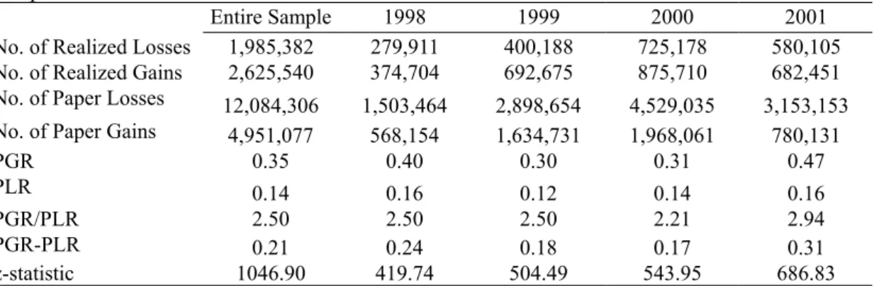
Table 2 compares the PGR and PLR for the entire data and the results partitioned by year. The results show that investors do sell a higher proportion of their winners than of their losers both for entire sample and for yearly breakdown. A one-tailed test of the null hypothesis that PGR≦PLR can be rejected with significant t-statistics. Note that the difference of PGR and PLR (0.21) in this study is much greater magnitude than that in Odean (0.05). On average, investors’ proportion of realizing gains is 2.5 times that of realizing losses. In each year the ratio of PGR to PLR falls in the range of 2.2 to 2.9.
To test the robustness of these results, we also conduct alternative tests. First of all, instead of assuming that independence exists at a transactional level we assume only that it exists at an account level. That is, the PGR and PLR are re-estimated for each account. The result still holds water for the disposition effect. Secondly, some possible choices of reference point for stocks are used for a subsample test, for example, the average purchase price, the highest purchase price, the first purchase price, or the most recent purchase price. The findings are essential the same for each choice. Furthermore, Lakonishok and Smidt (1986) suggest that investors might sell winners and hold on losers in an effort to rebalance their portfolios. An alternative test of using the subsample of selling the entire holding of stocks, which is less likely to be motivated by the desire of rebalancing, is investigated and results in similar
findings.
<<Insert Table 2 Here>>
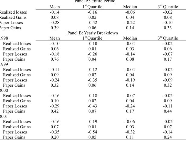
Table 3 reports the distribution of returns realized on stocks sold for a loss and stocks sold for a gain. It also reports the corresponding returns of stocks that could be but are not sold for a loss or a gain on the same days that other stocks in the same portfolio are sold.These stocks are classified as paper gains and paper losses. The results portray an interesting pattern that the returns of paper gains are much larger in extent than those of realized gains, and the returns of paper losses are also much larger in extent than those of realized losses. For example, for the entire period the average return on paper gains (39%) is much larger than that on realized gains (8%), and the average return on paper losses (-28%) is much larger in extent than that on realized losses (14%). The aforementioned sequence of returns on paper gains (losses) and realized gains (losses) sustains in each year. In Odean (1998) the average returns on paper gains, realized gains, paper losses, and realized losses are 46.6%, 27.7%, -39.3%, and –22.8%, respectively. This implies that investors in Taiwan are more impatient in tackling investment than their U.S. counterparts.
Even though in absolute- or relative term the counts of selling winners outweigh those of selling losers, the stocks that are not sold have potential returns of much greater magnitude than those are sold. This seems to contradict with the
disposition effect illustrating that the value function of an investor is concave in the domain of gains and convex in the domain of losses. For example, if people are risk adverse when they face gains, they should not have higher average returns on paper gains than on realized gains. Odean (1998) also had the same finding but did not offer further explanations. We doubt that there might be situations that people are not disposed in tackling their winners versus losers from investment. We will get back this issue in the later part.
<<Insert Table 3 Here>>
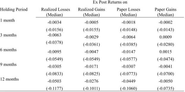
Even though the evidence from table 2 indicates that investors are more likely to realize gains than losses, it would be premature to draw conclusion of the disposition effect without further examination of the ex-post returns. The average returns in excess of the TSE value-weighted index to stocks that are sold for a loss or a gain, and to stocks that could be, but are not, sold for a loss or a gain are reported in table 4. Returns are measured over the holding periods of 1 month, 3-, 6-, 9-, and 12 months subsequent to the sales of a realized loss (gain) and subsequent to days on which sales of other stocks take place in portfolio of a paper loss (gain).
The results show that the average ex-post excess returns on paper losses are lower than those on realized gains for different holding periods, which is predicted by the disposition effect. However, the ex-post market-adjusted returns on realized gains are negative for different holding periods. Thus, investors hold their losers too long while not necessary sell their winners too soon.
<<Insert Table 4 Here>>
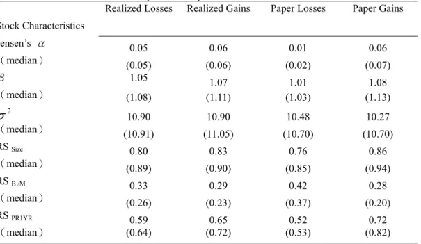
The general picture so far indicates that investors are disposed to asymmetric dealing with their winners verse losers, which is especially true for the relative counts of winners and losers. We would like to further explore the characteristics of stocks hold by individual investors. Table 5 summarizes the means and medians of the characteristics of interest including Jensen’sα, systematic risk (β), σ2, and the characteristics rank scores of size, book-to-market ratio, and stock prior year return. The characteristic rank score (RS) for a stock, referred to Chen, Jegadeesh, and Wermers (1999), is that stock’s percentile rank on that characteristic relative to all stocks covered by both TSE and OTC markets. The ith-ranked stock is assigned a rank score of (i-1)/(N-1), where N represents the number of the listed stocks in both TSE and OTC market.
The results show that the stocks traded for gains or losses, or stocks potentially can be traded for gains or losses have positive risk-adjusted returns. On average, the stocks held by individual investors are a little bit more risky than market portfolio. And the variance of returns of these stocks is around 10% to 11%. Investors are inclined to invest on large-cap- and growth stocks, as shown in the average rank scores of size and equity book-to-market ratio. The stocks realized or could be potentially realized as a gain have much higher prior-one-year return than those realized or potentially could be realized as a loss, implying the momentum effect on stock returns.
Odean (1998) found that tax-motivated selling in December could affect an investor’s disposition effect. However, investors in Taiwan are exempted from the taxes of realizing capital gains, and the yearend tax-motivated selling is less than an issue herein. In fact, the ratios of RGR to PLR in each month fall within a narrow range of 2.14 in April to 3.0 in November. Besides, some argue that people are in need of money at the time closing Chinese new year, usually occurs at January or February. Or people are prone to engage in selling stocks for paying taxes at the taxes paying month of April. However, the empirical results fail to support the aforementioned arguments.
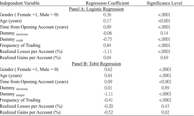
Except for the monthly effect, we would like to explore the factors that affect an investor’s attitude toward their winners and losers. The logistic and tobit regressions are used herein and the results are summarized in table 6. For the logistic regression the independent variable is assigned the value of 1 when PGR is greater than PLR, and 0 otherwise. The case of (PRG > PLR) is used to surrogate investors’ disposition toward their winners rather than losers, ceteris paribus. For the tobit regression the independent variable is the ratio of PGR to PLR.
Barber and Odean (2000) show that men are more overconfident, trade more excessively, and have lower net returns than women. Arithmetically, the disposition effect of women is expected to be higher than that of men since that the ratio of PGR to PLR is greater than 1 and that men are proved to trade more excessive than women. Take an invented case for example, if the realized gains, paper gains, realized losses, and paper losses of women are 3, 2, 2, and 2, respectively. The corresponding PGR, PLR, and the ratio of PGR to PLR are 3/5, 2/4, and 12/10 (or 1.2). Men are more excessively trading and have the realized gains, paper gains, realized losses, and paper losses of 4, 3, 3, and 3, respectively. The corresponding PGR, PLR, and the ratio of
PGR to PLR are 4/7, 3/6, and 24/21 (or 1.14). The gist is that a fraction of greater than 1 will decrease its value when the numerator and denominator are amplified with the same magnitude.
Psychologically, if self-confidence were a qualified proxy for decisiveness, a self-confident man with excessive trading would be less disposed to deal with their winners and losers. The first independent variable of interest is gender dummy that assigns the value of 1 for women and 0 for men. We expect to find that men are less disposed than women. An unreported result of univariate test by partitioning investors on gender indicates that the ratio of PGR to PLR is 1.86 for men and 2.24 for women.
The second independent variable of interest is the age of investors. Age is related to a man’s life-cycle style and his disposable income. A young man is supposed to have more disposable income, be more active, and be more willing to take riskier investment than an old one. Thus, he or she is less disposed to keeping losers too long. When the data is separated into quartiles based on investors age the proportions of PGR to PLR are 1.98, 199, 2.01 and 2.13 for each age quartile, respectively.
The third variable of interest is the time from opening account in the brokerage house that serves as a proxy for an investor’s experience. An inexperienced investor tends to a small-amount investor and is supposed to be more willing to assume his losses than an experienced one. Clearly, this proxy variable is not used without question since investors might have other accounts that are not part of the data set.
However, it is unlikely that the data set of partial investors’ portfolio will lead to systematical bias.
The next two independent variables are electronic dummy and margin dummy. The electronic dummy signifies that those who trade through electronic system are more willing to assume losses and have less extent of the disposition effect than those do not. The margin dummy is used to indicate that the margin-purchase or short-selling investors levering their positions through margin are more willing to assume losses and have less extent of the disposition effect.
The effect of trading frequency is ambivalent to the disposition effect. First of all, the infrequent investors tend to be patient traders. And their scant trading records more often than not are insufficient to vindicate the disposition effect. However, frequent traders are overconfident and less disposed to deal with their winners and losers. When the investors are equally divided into quartiles based on trading frequency, we found that the proportions of PGR to PLR are 1.70, 2.24, 2.15, and 1.83, respectively. Finally, two control variables, the return rate of realized gains and that of realized losses are utilized to explore whether an investor with higher realized gains (losses) would affect his preference for realizing gains or losses.
Basically, the results of the logistic regression and the probit regression verify our conjecture. Women are more likely to prefer to selling winners too soon and keeping losers too long than men. Aged and experienced investors have a higher
propensity to fall in the dictum of the disposition effect than young and inexperienced ones. The result also shows that the credit-account investors levering their position through margin are less disposed to asymmetrically deal with their winners and losers.
Note that trading frequency is positively related to the dummy (PGR>PLR) in the logistic regression, while negatively related to the ratio of PGR to PLR in the tobit regression. As mentioned above, trading frequency is less clear to the disposition effect in that infrequent trading records of investors are too scanty to vindicate the disposition effect while the frequent trading is connected to overconfidence with which investors are more willing to assume losses and less disposed to deal with winners and losers. The results of the electronic dummy and the returns of realized gains and losses are mixed supported.
<<Insert Table 6 Here>>
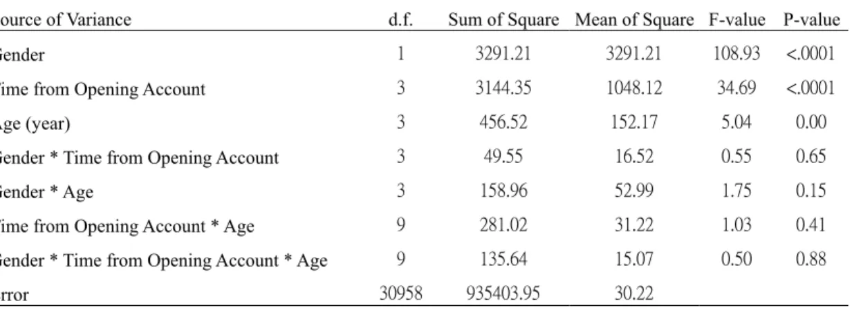
In table 7 we use the analysis of variance of PGR/PLR and the variables of interest to see if these variables are interactively related. The results show that gender, time from opening account, and age contribute to the explanation of the variance of PGR/PLR. The interaction of gender and age marginally contributes to the explanation of the variance of PGR/PLR with the significance level of 0.15. The result concludes a general picture that aged female is more inclined to asymmetrically deal with their winners than losers. Those aged female investors tend to be nonprofessional investors with limited knowledge and are east to be the pawns of the disposition effect.
<<Insert Table 7 Here>>
their sensitivity to higher trading cost at loser stock prices. Odean (1998) reports PGR and PLR for different price ranges and return ranges and finds that the disposition effect is sustainable for the results by partitioning on magnitude of return and price. From a different perspective, we would like to investigate whether investors are consistently the pawns of the disposition effect in facing different scenarios? Or they can be rationally dealing with their winners and losers under certain circumstances? In table 8 the data are equally partitioned into quartiles and reports the results of PGR, PLR, PRG-PLR, and PGR/PLR based on absolute value of return (panel A), stock price (panel B), and both absolute value of return and stock price (panel C)3.
The result in panel A shows that the PGR/PLR is less than 1 for the cases in the first- and fourth quartile. This implies that investors are not disposed to selling their winners too soon and keeping losers too long when their investment is deep in the money and deep out of the money (the fourth quartile), or when their investment falls within a narrow range of gains or losses (the first quartile). In facing gigantic losses, investors would trigger the self-control mechanism to bound losses within tolerable limit, and thus are less disposed to asymmetrical dealing with gains and losses. Those who confronted with huge gains from investment of stocks are men refraining from themselves realizing small gains, and thus are less disposed to gains and losses. In other words, self-abnegation accounts for the cases that investors in the high absolute return group are less disposed.
However, it is less clear why investors in low absolute return group are less disposed. According to Kanneman and Tversky’s prospect theory, people value function is defined on gains and losses rather than on levels of wealth. Thus the value
3 We also partition the sample into quartiles based on investor’s shareholding, dollar amount of
function is concave in the domain of gains and convex in the domain of losses. It also implies that people react differently to their winners and losers. Arguably, attitude change of an investor is most significant around the reference point or within a narrow range of return.
The result from panel B of partitioning by price corroborates the prediction of the disposition effect. In panel C we split the sample into 16 partitions based on the quartiles of absolute value of return and the quartiles of stock price. The results indicate that investors are less disposed when the absolute return is high and price is low, and when the absolute return is low and the stock price is high. For example, when the change of absolute return is greater than 10% and the price of stock is lower than $18.44 (the sample median) an investor’s proportion of realizing gains is lower than his proportion of realizing losses. Investors are also have higher proportion of realizing gains than losses when the change of absolute return is lower than 1% and the stock price is higher than $18.44.
<<Insert Table 8 Here>>
V. Conclusion
This paper investigates the behavior of individual investors from a data set of 53,680 accounts covering 10,883,473 transaction records. The results show that investors in Taiwan exhibit disposition effect to an extent more than the U.S. investors. On average, the proportion of realizing gains is 2.5 times that of realizing losses. And the average excess returns on paper losses are lower than those on realized gains for the holding periods of 1-,3-,6-, 9-, and 12 months subsequent to the sales of a realized gain and subsequent to days on which sales of other stocks take place in portfolio of a
paper loss.
Moreover, logistic regression as well as tobit regression are used to investigate the characteristics that affect an investor’s inclination on realizing gains than losses. The results indicate that aged female, who tends to be a nonprofessional investor with limited knowledge, is more inclined to asymmetrically deal with their winners than losers. In contrast, the credit-account investors levering their position through margin are less to be pawns of the disposition effect.
We also explore the situations that affect an investor’s attitude to deal with his winners and losers by partitioning sample based on the quartiles of absolute return and stock price. PGR/PLR is less than 1 for the high-absolute-return quartiles, indicating that investors trigger the self-control mechanism in order to bound losses within tolerable limit and also forbear from realizing small gains. However, it is less clear why investors in low-absolute-return group are also less disposed.
The potential contribution of this study is to explore the characteristics of an investor, i.e. gender and age, and the conditions faced by an investor, i.e. high- and low-absolute return, affect his/her attitude to deal with winners and losers. One interesting finding is that men, who tend to be overconfident investors engaging excessive trading, are less disposed to deal with gains and losses. Exploring the connection between overconfidence and the disposition effect merits further research efforts.
References
Andreassen, P., 1988, Explaining the price-volume relationship: The difference between price changes and changing prices, Organizational Behavior and Human Decision Processes 41, 371--389.
Badrinath, S., and Lewellen W., 1991, Evidence on tax-motivated securities trading behavior, Journal of Finance 46, 369--382.
Chen, H.L., Jegadeesh N., and Wermers R., 2000, The value of active mutual fund management: An examination of the stockholdings and traded of fund managers, Journal of Financial and Quantitative Analysis 35, 343--368.
Harris, L., 1988, Discussion of predicting contemporary volume with historic volume at differential price levels: Evidence supporting the disposition effect, Journal of Finance 43, 698--699.
Kahneman, D., and Tversky A., 1979, Prospect theory: An analysis of decision under risk, Econometrica 46, 263--291.
Lakonishok, J., and Smidt S., 1986, Volume for winners and losers: Taxation and other motives for stock trading, Journal of Finance 41, 951--974
Odean, T., 1998, Are investors reluctant to realize their losses?, Journal of Finance 53, 1775--1798.
Schlarbaum, G., Lewellen W., and Lease R., 1978, Realized returns on common stock investments: The experience of individual investors, Journal of Business 51, 299--325.
Shefrin, H. and Statman M., 1985, The disposition to sell winners too early and ride losers too long: Theory and evidence, Journal of Finance 40, 777--790
Thaler, R., 1985, Mental accounting and customer choice, Marketing Science 4, 199--214
Table 1 Summary Statistics of Sample
This table reports summary statistics of a sample obtained from a renowned securities brokerage house. From all accounts active beginning from January 1998 and ending September 2001, 53,680 customer accounts are randomly selected. In total there are 10,883,473 records, each record is made up of an account identifier, the trade date, the trading type (cash trading, long (short) margin trading, margin call), a buy-sell indicator, a branch identifier, the internal number for securities traded, the quantity traded, trading price, the principal amount, and the transaction taxes. Among the attributes of accounts the first-, second-, and third quartiles of the years of age, the time from opening account, and the number of trades are reported accordingly.
201 Below 13 13,468 25.1 14 – 48 13,526 25.2 49 – 153 13,330 24.8 Number of Trades Above 154 13,356 24.9 53,680 100﹪ Yes 14,347 26.7
Trading through Margin
No 39,333 73.3
53,680 100﹪ Account Attribute Mean Number Percentage(﹪) Total
Male 26,244 48.9 Gender Female 27,436 51.1 53,680 100﹪ 39 Below 31 13,415 25.0 31 – 38 13,424 25.0 38 – 47 13,415 25.0 Years of Age Above 47 13,425 25.0 53,679 100﹪ 25.2 Below 16 13,440 25.04 16 – 28 13,430 25.02 28 – 46 13,393 24.95 Time from Opening Account
(months)
Above 46 13,417 24.99
53,680 100﹪
Yes 29,802 55.5
Trading through Electronic System
No 23,878 44.5
53,680 100﹪
Table 2 PGR and PLR for Entire Data and Partitioned by Year
This table compares the Proportion of Gains Realized (PGR) to Proportion of Losses Realized (PLR) for the aggregate sample and for the sample partition by year, where PGR is the number of realized gains divided by the number of realized gains plus the number of paper (unrealized) gains, and PLR is the number of realized losses divided by the number of realized losses plus the number of paper (unrealized) losses, according to Odean (1998). Each day that a sale takes places, the selling price for each stock sold to its average purchase price between the latest two selling days are compared and determined whether that stock sold is recognized as a gain or loss. For those stocks in portfolio but not sold in that day, if both its daily high and low are above (below) its average purchase price between the latest two selling days it is counted as a paper gain (loss); if its average price lies between the high and low, neither a gain or loss is counted. On days when no sales take place in an account, no gains or losses, realized or paper, are counted. Realized gains, paper gains, realized losses, and paper losses are simply the counts across all accounts over the sampling period beginning from January 1998 and ending September 2001. The z-statistics test the null hypotheses that the differences in proportions are equal to zero assuming that all realized gains, paper gains, realized losses, and paper losses result from independent decision.
Entire Sample 1998 1999 2000 2001
No. of Realized Losses 1,985,382 279,911 400,188 725,178 580,105 No. of Realized Gains 2,625,540 374,704 692,675 875,710 682,451 No. of Paper Losses 12,084,306 1,503,464 2,898,654 4,529,035 3,153,153 No. of Paper Gains 4,951,077 568,154 1,634,731 1,968,061 780,131
PGR 0.35 0.40 0.30 0.31 0.47
PLR 0.14 0.16 0.12 0.14 0.16
PGR/PLR 2.50 2.50 2.50 2.21 2.94
PGR-PLR 0.21 0.24 0.18 0.17 0.31
Table 3: Average Returns
This table reports the mean, 1st, 2nd (median), and 3rd quartile returns realized on stocks sold for a loss
and stocks sold for a gain. It also reports the corresponding returns of stocks that could be but are not sold for a loss or a gain on the same days that other stocks in the same portfolio are sold. These stocks are classified as paper gains and paper losses. Panel A reports all accounts over the entire period, while panel B reports the returns of yearly breakdown. The realized return is the difference between the selling price and its average cost divided by its average cost. The paper return is the difference between the closing price of unsold stocks and its average cost divided by its average cost.
Panel A: Entire Period
Mean 1st Quartile Median 3rd Quartile
Realized losses -0.14 -0.16 -0.06 -0.02
Realized Gains 0.08 0.02 0.04 0.08
Paper Losses -0.28 -0.42 -0.22 -0.10
Paper Gains 0.39 0.06 0.14 0.33
Panel B: Yearly Breakdown
1998 Mean 1st Quartile Median 3rd Quartile
Realized losses -0.10 -0.10 -0.04 -0.02 Realized Gains 0.06 0.01 0.03 0.06 Paper Losses -0.18 -0.26 -0.14 -0.07 Paper Gains 0.76 0.04 0.08 0.17 1999 Realized losses -0.11 -0.12 -0.04 -0.02 Realized Gains 0.09 0.02 0.04 0.09 Paper Losses -0.24 -0.35 -0.19 -0.09 Paper Gains 0.32 0.06 0.14 0.32 2000 Realized losses -0.16 -0.18 -0.07 -0.02 Realized Gains 0.10 0.02 0.04 0.09 Paper Losses -0.29 -0.43 -0.24 -0.11 Paper Gains 0.42 0.07 0.17 0.44 2001 Realized losses -0.16 -0.19 -0.06 -0.02 Realized Gains 0.07 0.01 0.03 0.07 Paper Losses -0.35 -0.54 -0.32 -0.14 Paper Gains 0.20 0.05 0.11 0.24
Table 4 Ex Post Returns
This table reports average returns in excess of the TSE value-weighted index to stocks that are sold for a loss (realized losses) or a gain (realized gains), and to stocks that could be, but are not, sold for a loss (paper losses) and a gain (paper gain). Returns are measured over the holding periods of 1 month, 3-, 6-, 9-, and 12 months subsequent to the sales of a realized loss (gain) and subsequent to days on which sales of other stocks take place in portfolio of a paper loss (gain). The medians of ex post returns are provided in parentheses.
Ex Post Returns on Holding Period Realized Losses
(Median) Realized Gains (Median) Paper Losses (Median) Paper Gains (Median) 1 month -0.0034 -0.0005 -0.0018 -0.0002 (-0.0156) (-0.0155) (-0.0148) (-0.0143) 3 months -0.0063 -0.0029 -0.0064 0.0009 (-0.0378) (-0.0361) (-0.0385) (-0.0280) 6 months -0.0095 -0.0047 -0.0147 0.0015 (-0.0549) (-0.0549) (-0.0577) (-0.0474) 9 months -0.0305 -0.0171 -0.0307 -0.0041 (-0.0833) (-0.0825) (-0.0773) (-0.0700) 12 months -0.0503 -0.0276 -0.0449 -0.0050 (-0.1177) (-0.1011) (-0.1060) (-0.0735)
Table 5 Stock Characteristics
This table reports the means and medians of the characteristics of stocks that are sold for a loss (gain) and stocks that could be, but are not, sold for a loss (gain). Jensen’s α and stock β are obtained from market model in the sampling period prior to the sale that is recognized as a loss (gain) takes place. σ2 is estimated from the daily returns of stocks before sold for a loss (gain). The characteristic rank score (RS) for a stock is that stock’s percentile rank on that characteristic relative to all stocks covered by both TSE and OTC markets. The ith-ranked stock is assigned a rank score of
(i-1)/(N-1), where N represents the number of the listed stocks in both TSE and OTC market. The characteristics of interest in this study are equity size (Size), equity book value to market value (B/M), and prior one-year return (PR1YR). The characteristic ranks of stock sold are equally weighted. The medians of stock characteristics are provided in parentheses.
Realized Losses Realized Gains Paper Losses Paper Gains
Stock Characteristics Jensen’s α 0.05 0.06 0.01 0.06 (median) (0.05) (0.06) (0.02) (0.07) β 1.05 1.07 1.01 1.08 (median) (1.08) (1.11) (1.03) (1.13) 2 σ 10.90 10.90 10.48 10.27 (median) (10.91) (11.05) (10.70) (10.70) RS Size 0.80 0.83 0.76 0.86 (median) (0.89) (0.90) (0.85) (0.94) RS B /M 0.33 0.29 0.42 0.28 (median) (0.26) (0.23) (0.37) (0.20) RS PR1YR 0.59 0.65 0.52 0.72 (median) (0.64) (0.72) (0.53) (0.82)
Table 6 Logistic- and Tobit Regressions
The independent variable of the logistic regression is assigned the value of 1 when PGR is greater than PLR, and 0 otherwise. The independent variable of tobit regression is the ratio of PGR to PLR. The regressions are conducted via per account basis. The dependent variables for logistic- and tobit regressions includes the age of investor, time from opening account, Dummy electronic , Dummy credit ,
frequency of trading, realized losses of an account, an realized gains of an account. Among them Dummy electronic is assigned the value of 1 when the transaction of account is executed through
electronic system, and 0 otherwise. Dummy margin is assigned value of 1 when the account is a credit
account, and 0 otherwise. Panel A reports the result of logistic regression, while panel B reports the result of tobit regression. The regression coefficients and significance level are provided in the second and third column.
Independent Variable Regression Coefficient Significance Level Panel A: Logistic Regression
Gender ( Female =1, Male = 0) 0.36 <.0001
Age (years) 0.17 <0.001
Time from Opening Account (years) 0.09 <.0001
Dummy electronic -0.06 0.14
Dummy credit -0.75 <.0001
Frequency of Trading 0.84 <.0001
Realized Losses per Account (%) -1.11 <.0001
Realized Gains per Account (%) 0.04 0.69
Panel B: Tobit Regression
Gender ( Female =1, Male = 0) 0.62 <.0001
Age (years) 0.84 <.0001
Time from Opening Account (years) 0.09 <0.001
Dummy electronic 0.01 0.89
Dummy margin -1.11 <.0001
Frequency of Trading -0.41 <.0001
Realized Losses per Account (%) -0.20 0.43
Table 7 Analysis of Variance
The analysis of variance is based on the ratio of PGR to PLR (PGR/PLR) to the characteristic variables of account, including gender, time from opening account (equally divided into quartiles), age of investors (equally divided into quartiles), and the interactions of variables. Degree of freedom (d.f.), sum of square, mean of square, F-value, and p-value for each variable (or interaction of variables) are provided accordingly.
Source of Variance d.f. Sum of Square Mean of Square F-value P-value
Gender 1 3291.21 3291.21 108.93 <.0001
Time from Opening Account 3 3144.35 1048.12 34.69 <.0001
Age (year) 3 456.52 152.17 5.04 0.00
Gender * Time from Opening Account 3 49.55 16.52 0.55 0.65
Gender * Age 3 158.96 52.99 1.75 0.15
Time from Opening Account * Age 9 281.02 31.22 1.03 0.41
Gender * Time from Opening Account * Age 9 135.64 15.07 0.50 0.88
Table 8 PGR and PLR Partitioned by Return and Price
This table compares the aggregate Proportion of Gains Realized (PGR) to the aggregate Proportion of Losses Realized (PLR), where PGR is the number of realized gains divided by the number of realized gains plus the number of paper (unrealized) gains, and PLR is the number of realized losses divided by the number of realized losses plus the number of paper (unrealized) losses. For all accounts in the sampling period beginning from January 1998 and ending September 2001, the data are equally partitioned into quartiles based on absolute value of return in Panel A, on stock price in Panel B, and both absolute value of return and stock price in Panel C. The t-statistics test the null hypotheses that the differences in proportions are equal to zero assuming that all realized gains, paper gains, realized losses, and paper losses result from independent decisions.
Panel A: Partitioned by Return
|R|≤0.01 0.01<|R|≤0.1 0.1<|R|≤0.65 0.65<|R| Realized losses 280,290 1,009,797 601,139 93,705 Realized Gains 380,656 1,715,152 497,450 32,282 Paper Losses 93,863 2,921,976 8,125,508 942,959 Paper Gains 171,492 1,825,258 2,393,065 561,262 PGR 0.69 0.48 0.17 0.05 PLR 0.75 0.26 0.07 0.09 PGR/PLR 0.92 1.85 2.43 0.60 PGR-PLR -0.06 0.23 0.10 -0.04 z-statistic -63.30 659.59 433.67 -88.37
Panel B: Partitioned by Price
P≤11.00 11.00<P≤18.44 18.44<P≤30.95 30.95<P Realized losses 230,079 298,699 591,979 864,174 Realized Gains 111,167 307,398 769,625 1,437,350 Paper Losses 766,308 1,837,237 3,364,208 6,116,553 Paper Gains 324,002 723,758 1,585,450 2,317,867 PGR 0.26 0.30 0.33 0.38 PLR 0.23 0.14 0.15 0.12 PGR/PLR 1.13 2.14 2.20 3.17 PGR-PLR 0.02 0.16 0.18 0.26
Panel C: Partitioned by Return and Price
|R|≤0.01 0.01<|R|≤0.1 0.1<|R|≤0.65 0.65<|R| P≤11.00 PGR 0.53 0.43 0.13 0.02 PLR 0.49 0.26 0.14 0.36 PGR/PLR 1.08 1.65 0.93 0.06 PGR-PLR 0.04 0.16 -0.01 -0.34 z-statistic 7.88 109.48 -8.69 -293.54 11.00<P≤18.44 PGR 0.68 0.45 0.12 0.02 PLR 0.72 0.09 0.32 0.03 PGR/PLR 0.94 5.00 0.38 0.67 PGR-PLR -0.04 0.36 -0.19 -0.01 z-statistic -14.44 473.44 -209.46 -18.79 18.44<P≤30.95 PGR 0.72 0.48 0.15 0.02 PLR 0.79 0.26 0.08 0.01 PGR/PLR 0.91 1.85 1.88 2.00 PGR-PLR -0.07 0.22 0.07 0.01 z-statistic -42.53 354.17 168.32 18.25
30.95<P PGR 0.68 0.50 0.21 0.11 PLR 0.75 0.53 0.04 0.00 PGR/PLR 0.91 0.94 5.25 69.57 PGR-PLR -0.07 -0.03 0.17 0.11 z-statistic -52.67 -49.81 474.53 166.77