有全方位監控之多輛電腦視覺自動車的最佳安全巡邏之研究

全文

(1)有全方位監控之多輛電腦視覺自動車的最佳安全巡邏之研究. 研究生：陳倖嘉. 指導教授：蔡文祥. 教授. 國立交通大學多媒體工程研究所. 摘要本論文提出利用多輛視覺型自動車執行安全巡邏工作的系統。我們假設巡邏環境的地板形狀是由矩形區塊所組成，並採用兩輛裝設有攝影機的自動車，以及兩部固定於天花板的魚眼鏡頭攝影機做為實驗平台。我們提出了一項獲取未知環境資訊的方法，可得到組成環境的所有矩形區域、導航自動車的轉折點、每組監控點間的距離與巡邏路徑。利用這些資訊可使自動車在航行時，不會與牆壁產生擦撞。另外，針對相機校正的問題，我們亦提出一項結合影像內插的點對應方法，利用多組二維影像與三維真實空間的對應點與影像內插法，去求得點在扭曲影像中的實際正確位置。此外，為了提高相機校正的精準度，我們也提出一項快速求取多組對應點的方法。藉由這些方法，我們可利用固定於天花板上的俯視攝影機來學習自動車相對於監控物品的位置與朝向，並利用此資訊來執行安全巡邏的工作。再者，我們也用俯視攝影機來定位與監控自動車的移動行為。而為了使得本系統有較好效益，我們則提出一項具有優化隨機與工作量平衡特性的路徑規劃方法，來分配巡邏路徑給各自動車，縮短完成每輪巡邏工作所花費的時間，進而提高環境中的安全程度。最後，由於本系統中所採用的自動車數量不只一台，所以我們提出了即時避碰的技巧，根據可能產生碰撞的路線狀況，自動產生可行駛的避碰路線。實驗結果證明我們所提出的這些方法是可行而且有效的。 i.

(2) A Study on Optimal Security Patrolling by Multiple Vision-Based Autonomous Vehicles with Omni-Monitoring. Student: Hsing-Chia Chen. Advisor: Prof. Wen-Hsiang Tsai, Ph. D.. Institute of Multimedia Engineering, College of Computer Science National Chiao Tung University. ABSTRACT A multiple vision-based vehicle system for security patrolling in an indoor environment, whose floor shape is composed of rectangular regions, is proposed. Two autonomous vehicles controllable by wireless communication and equipped with cameras, as well as two cameras with fish-eye lenses fixed on the ceiling, are used as a. test. bed.. To. acquire. information. of. an. unknown. environment,. an. environment-information calculation method is proposed for obtaining all rectangular regions composing the floor shape of the environment, the turning points for navigation, all distances between monitored objects, and the patrolling paths. These data enable the vehicles to navigate without collisions with walls. Also, a point-correspondence technique integrated with an image interpolation method is proposed for camera calibration. By a technique of finding corresponding points in 2-D image and 3-D global spaces as well as an image interpolation method, the correct positions of interesting feature points can be obtained from the warped images captured by the cameras with fish-eye lenses. Besides, a faster point-correspondence technique is proposed to obtain abundant corresponding points that yield better calibration accuracy. With this camera calibration technique, the cameras on the ii.

(3) ceiling can be utilized to learn the poses of the vehicles with respect to monitored objects. Also, the vehicles are taught where and in which direction to perform the security monitoring task, in which the position information is used to guide the vehicles. Additionally, the top-view cameras can also be utilized to locate the vehicles and monitor vehicle activities in the navigation phase. An optimal randomized and load-balanced path planning method is proposed as well, which requires shorter time to accomplish object monitoring in one session and provides higher degrees of patrolling security. Because the number of the vehicles used in this study is more than one, a real-time collision avoidance technique is also proposed. According to the state of path-intersecting, feasible alternative paths for the vehicles can be obtained. Good experimental results show the flexibility and feasibility of the proposed methods for the application of multiple-vehicle security patrolling.. iii.

(4) ACKNOWLEDGEMENTS I am in hearty appreciation of the continuous guidance, discussions, support, and encouragement received from my advisor, Dr. Wen-Hsiang Tsai, not only in the development of this thesis, but also in every aspect of my personal growth. Thanks are due to Mr. Chih-Jen Wu, Mr. Che-Wei Lee, Miss Shung-Yung Tsai, Mr. Guan-Lin Huang, and Mr. Jiun-Tsung Wang for their valuable discussions, suggestions, and encouragement. Appreciation is also given to the colleagues of the Computer Vision Laboratory in the Institute of Computer Science and Engineering at National Chiao Tung University for their suggestions and help during my thesis study. Finally, I also extend my profound thanks to my family for their lasting love, care, and encouragement. I dedicate this dissertation to my beloved parents.. iv.

(5) CONTENTS ABSTRACT..................................................................................................................ii ACKNOWLEDGEMENTS .......................................................................................iv CONTENTS..................................................................................................................v LIST OF FIGURES ...................................................................................................vii LIST OF TABLES........................................................................................................x Chapter 1 1.1 1.2 1.3 1.4 1.5. Introduction..............................................................................................1 Motivation of Study ...................................................................................1 Survey of Related Studies ..........................................................................2 Overview of Proposed Approach ...............................................................4 Contributions..............................................................................................8 Thesis Organization ...................................................................................9. Chapter 2 System Configuration and Navigation Principles...............................10 2.1 Introduction..............................................................................................10 2.2 System Configuration ..............................................................................12 2.2.1 Hardware configuration ....................................................................14 2.2.2 Software configuration......................................................................17 2.3 Learning Principle and Proposed Process................................................17 2.4 Vehicle Guidance Principle and Proposed Process..................................20 Chapter 3 Learning Strategies for Navigation by Semi-automatic Driving .......22 3.1 Ideas of Proposed Techniques Used in Learning .....................................22 3.2 Calibration of Top-View Omni-Cameras with Fish-Eye Lenses .............23 3.2.1 Review of Conventional Camera Calibration Technique .................24 3.2.2 Proposed Calibration Technique .......................................................25 3.3 Information for Security Patrolling..........................................................32 3.3.1 Proposed techniques of learning patrolling environment .................32 3.3.2 Learning of poses of vehicles with respect to monitored objects .....41 Chapter 4 Security Patrolling by Multiple Vehicle Navigation............................45 4.1 Introduction to Concepts in Proposed Systems .......................................45 4.1.1 Randomized patrolling......................................................................45 4.1.2 Optimal path......................................................................................46 4.1.3 Load balance .....................................................................................46 4.1.4 Top-view omni-monitoring ...............................................................46 4.1.5 Path correction by top-view monitoring omni-camera .....................47 v.

(6) 4.2. Proposed Techniques Used in Patrolling .................................................48 4.2.1 Optimal randomized patrolling paths for all vehicles.......................48 4.2.2 Guidance of vehicles by localization and monitoring using top-view omni-cameras..........................................................................................52 4.2.3 Avoiding collisions between vehicles ...............................................63 4.3 Detailed Process for Security Patrolling by Vehicle Navigation .............63 Chapter 5 Planning of Optimal Randomized Patrolling Paths for Vehicles.......68 5.1 Introduction..............................................................................................68 5.2 Calculation of Paths between Monitoring Points by Dijkstra’s Algorithm ................................................................................................................69 5.2.1 Review of Dijkstra’s algorithm.........................................................69 5.2.2 Proposed technique for generation of partial patrolling paths ..........70 5.3 Calculation of Optimal Randomized Patrolling Paths by Finding Hamiltonian Paths...................................................................................76 5.3.1 Review of Traveling-Salesman Problem (TSP) ................................76 5.3.2 Proposed technique for generation of complete patrolling paths......77 Chapter 6 Collision Avoidance between Vehicles ..................................................81 6.1 Introduction..............................................................................................81 6.2 Detection of Collisions ............................................................................81 6.3 Proposed Collision Avoidance Techniques ..............................................82 6.3.1 Collision avoidance on intersecting paths.........................................82 6.3.2 Collision avoidance on non-intersecting paths .................................89 Chapter 7 7.1 7.2 7.3. Experimental Results and Discussions.................................................95 Experimental Results of Simulation of Patrolling ...................................95 Experimental Results of Patrolling in Real Environment......................101 Discussions ............................................................................................108. Chapter 8 Conclusions and Suggestions for Future Works ............................... 110 8.1 Conclusions............................................................................................ 110 8.2 Suggestions for Future Works................................................................ 112 References ................................................................................................................. 114. vi.

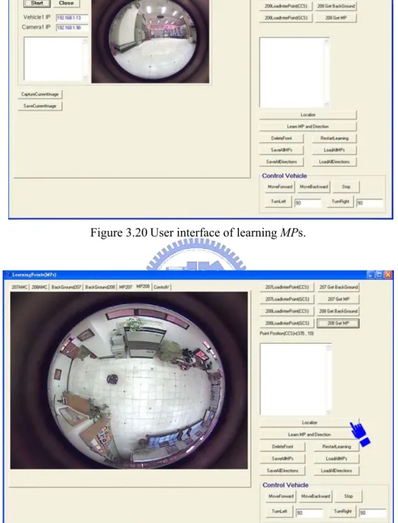
(7) LIST OF FIGURES Figure 1.1 Flowchart of learning process of proposed system. .....................................5 Figure 1.2 Flowchart of navigation of proposed system................................................7 Figure 2.1 The vehicle used in this study is equipped with a camera. (a) A perspective view of the vehicle. (b) A front view of the vehicle. (c) A side view of the vehicle. ..................................................................................................... 11 Figure 2.2 The vehicle system used in this study. (a) A Pioneer 3-DX vehicle. (b) A WiBox. (c) An Axis 207MW camera. ......................................................13 Figure 2.3 Structure of proposed system. ....................................................................15 Figure 2.4 The camera system used in this study. (a) A perspective view of the camera. (b) A front view of the camera. (c) A left-side view of the camera..........16 Figure 2.5 Flowchart of proposed learning process.....................................................19 Figure 2.6 Flowchart of proposed navigation process. ................................................21 Figure 3.1 Calculating quadratic curves. .....................................................................27 Figure 3.2 Finding all corresponding points. ...............................................................29 Figure 3.3 Point I in a distortion image. ......................................................................30 Figure 3.4 A relation between the image taken by the omni-camera and the global space.........................................................................................................31 Figure 3.5 Intersections of L and the boundaries of the area. ......................................33 Figure 3.6 Setting a line segment l...............................................................................34 Figure 3.7 Scanning the line segment l to the left........................................................35 Figure 3.8 Scanning the line segment l to the right. ....................................................35 Figure 3.9 The right part of points a and b is not an inner range.................................36 Figure 3.10 The right part of points a and b is an inner range.....................................37 Figure 3.11 A patrolling area........................................................................................37 Figure 3.12 The first rectangular region. .....................................................................38 Figure 3.13 The second rectangular region..................................................................38 Figure 3.14 The third rectangular region. ....................................................................38 Figure 3.15 The fourth rectangular region. ..................................................................39 Figure 3.16 The fifth rectangular region......................................................................39 Figure 3.17 The sixth rectangular region. ....................................................................39 Figure 3.18 The seventh rectangular region.................................................................40 Figure 3.19 All turning points in the area. ...................................................................41 Figure 3.20 User interface of learning MPs.................................................................42 Figure 3.21 Before localizing the vehicle. ...................................................................42 Figure 3.22 Localizing the vehicle...............................................................................43 Figure 3.23 The vehicle in front of a monitored object. ..............................................44 vii.

(8) Figure 4.1 A flowchart of determining all paths for vehicles. .....................................52 Figure 4.2 Coordinate systems used in this study. (a) ICS (b)GCS (c)VCS................54 Figure 4.3 Vehicle localization from a top-view omni-camera....................................55 Figure 4.4 A background image taken by a top-view omni-camera. ...........................57 Figure 4.5 A foreground taken by a top-view omni-camera. .......................................57 Figure 4.6 Finding the position of a vehicle. (a) A binary image which is part of the image shown in Figure 4.3. (b) Erosion of (a) with a square mask. (c) Dilation of (b) with a square mask. (d) The connected component of (c) and the computed centroid (the white circle)...........................................58 Figure 4.7 Illustration of direction angles of the vehicle. ............................................60 Figure 4.8 Flowchart of localizing and monitoring vehicles. ......................................62 Figure 4.9 A direction angle θV. (a) Left ( 0 ≤ θ v ≤ π ). (b)Right ( -π ≤ θ v ≤ 0 )............64 Figure 4.10 The relation between θ and θV..................................................................64 Figure 4.11 Flowchart of Navigation and monitoring tasks. .......................................67 Figure 5.1 A patrolling environment. ...........................................................................72 Figure 5.2 The graph G from Figure 5.1......................................................................72 Figure 5.3 The first cycle. ............................................................................................73 Figure 5.4 The second cycle. .......................................................................................73 Figure 5.5 The third cycle. ...........................................................................................74 Figure 5.6 The fourth cycle..........................................................................................74 Figure 5.7 The fifth cycle.............................................................................................75 Figure 5.8 The sixth cycle............................................................................................75 Figure 5.9 The seventh cycle. ......................................................................................76 Figure 5.10 A patrolling environment..........................................................................78 Figure 5.11 A complete undirected graph G = (V, E). .................................................79 Figure 6.1 An intersection I on the paths of two vehicles............................................83 Figure 6.2 Passing point P is in the outer region. ........................................................85 Figure 6.3 The alternative path is not feasible. ............................................................85 Figure 6.4 The alternative path is not feasible. ............................................................86 Figure 6.5 An included angle θ between V Æ G and V Æ P. ......................................89 Figure 6.6 Alternative paths at a non-intersecting state...............................................90 Figure 6.7 The passing point P is too far. ....................................................................91 Figure 6.8 A passing point P at a non-intersecting state. .............................................92 Figure 6.9 P is too far...................................................................................................92 Figure 6.10 P2 is not in the rectangular region R.........................................................93 Figure 7.1 A simulated patrolling environment. ..........................................................96 Figure 7.2 Path planning for the two vehicles in a session..........................................97 viii.

(9) Figure 7.3 Path planning for the two vehicles in the next session...............................98 Figure 7.4 Collision avoidance of non-intersecting paths. ........................................100 Figure 7.5 Collision avoidance of intersecting paths.................................................101 Figure 7.6 The view of the first top-view omni-camera. ...........................................103 Figure 7.7 The view of the second top-view omni-camera........................................105 Figure 7.8 The security patrolling task. (a) Images captured in the learning phase. (b) Images captured in the navigation phase. ..............................................106 Figure 7.9 The security patrolling task. (a) Images captured in the learning phase. (b) Images captured in the navigation phase. (continued)...........................107. ix.

(10) LIST OF TABLES Table 5.1 Distances and passing turning points between every pair of monitoring points........................................................................................................78 Table 7.1 The table of time comparisons where O and X means conducted or not, respectively. .............................................................................................99 Table 7.2 Mechanical errors of the vehicle. ...............................................................102 Table 7.3 Errors of the first top-view omni-camera...................................................104 Table 7.4 Errors of the second top-view omni-camera. .............................................105. x.

(11) Chapter 1 Introduction. 1.1 Motivation of Study Applications of intelligent robots are increasing gradually. An autonomous vacuum cleaner is a famous instance. The autonomous vehicle used in this research is also a robot, but it can only move. In order to add more ability to it, the vehicle is equipped with a camera. With the camera and its movement, the view of the vehicle is extended to a wider range. Such a kind of vision-based autonomous vehicle can perform more complicated tasks, such as security patrolling. It also can replace human beings to do dangerous or dreary works, for example, unknown object clipping, interoffice document delivering, etc. A traditional security surveillance system is passive and restricted by its fixed position. The autonomous vehicle utilized to assist a security surveillance system can send an alert message to the security center actively when it detects an abnormal state. This provides more efficient and reliable security protection. Security patrolling by multiple vision-based autonomous vehicles is more efficient than by one, because less time is taken to complete one session of patrolling all monitored objects. An additional advantage is that the shorter time interval between two objects patrolled increases the degree of security. To have more benefits, a good planning of patrolling paths for all autonomous vehicles is important. Randomization, optimization, and load balancing are three critical principles that influence path planning. Autonomous vehicles patrolling 1.

(12) randomly make thieves have no idea about when an object is not monitored by any vehicle. Optimal paths and load balances among all vehicles can decrease the time for all monitored objects to be patrolled once. In order that an autonomous vehicle can carry out the patrolling task without any manpower, it has to be guided smartly. Ideas of learning artificial landmarks or specific scene features in the environment and locating the vehicle by landmark or feature matching have been developed intensively in the past decade. But most of them are restricted to be applicable in ideal environments, such as pure-colored backgrounds. Therefore, a top-view omni-camera with a fish-eye lens is utilized in this study to widen the applicable environment. The camera not only can locate autonomous vehicles but also can check ceaselessly whether they are still under control. As a summary, our research goal in this study is to develop an autonomous vehicle security patrolling system with the following capabilities: 1.. navigating automatically in environments whose floor shape is composed of rectangular regions;. 2.. monitoring and locating autonomous vehicles by top-view omni-cameras;. 3.. avoiding collisions between vehicles;. 4.. patrolling randomly; and. 5.. planning optimal paths and balanced loads for all autonomous vehicles.. 1.2 Survey of Related Studies In order to make autonomous vehicles navigate along a correct path, the vehicle location is the most vital information. Traditionally, an autonomous vehicle is 2.

(13) equipped with an odometer to measure the current location of the vehicle. However, the vehicle usually suffers from incremental mechanic errors. Thus we need a technique of vehicle location estimation to correct the mechanic error in the navigation session. For vehicle calibration, the geometric shapes of object boundaries [1, 2] or those labeled by users are utilized frequently [3, 4]. Furthermore, natural landmarks, such as house corners [5, 6], and the SIFT features of images [7] are also used in the techniques of vehicle calibration. In recent years, techniques of integrating laser range finders with conventional imaging devices have been proposed [8, 9]. In this study, a top-view omni-camera with a fish-eye lens is utilized to locate an autonomous vehicle. The camera must be calibrated before being used. Traditionally, we must calculate intrinsic and extrinsic parameters of the camera in order to obtain a projection matrix for transforming points between 2-D image and 3-D global spaces. A point-correspondence technique integrated with an image interpolation method is proposed, which is inspired by a technique coming from Lai and Tsai [10]. Because the camera is equipped with a fish-eye lens, images captured by it are warped. Winters and Santo-Victor [11] proposed a method for calibrating warped panoramic images. However, we can obtain a correct coordinate point directly by the camera calibration technique proposed by us. Path planning is an important topic for the security patrolling by multiple vehicles. Many methods for this aim have been proposed in [12, 13, 14]. Besides, load balancing among all vehicles also need to be paid attention. Hert and Richards [15] proposed a method of using a polygon partitioning algorithm to achieve this objective. In this study, we propose a technique of calculating optimal and load-balanced paths in terms of some guidance points where vehicles perform security monitoring tasks. The idea of using guidance points comes from a learning method proposed by Chen 3.

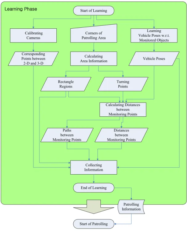
(14) and Tsai [16]. While vehicles navigate, collisions between vehicles must be avoided. Some methods [17, 18, 19] have been proposed to produce collision-free paths. To carry out optimal patrolling, we use the concept of the traveling salesman problem (TSP). Some methods for solving the TSP can be found in [20, 21, 22].. 1.3 Overview of Proposed Approach In this study, it is desired to develop a multiple vision-based autonomous vehicle system for security patrolling in an environment whose floor shape is composed of rectangular regions. In order to achieve this purpose, information about the environment, monitoring positions, and vehicle localization is quiet important. Therefore, some methods which can assist to acquire all of the above information are proposed and are roughly described in following. With such information, a technique which makes multiple vision-based autonomous vehicles navigate on correct paths without collisions and perform assigned security patrolling tasks is proposed. We divide the work conducted by the system into two phases: the learning phase and the navigation phase. They are illustrated in Figure 1.1 and Figure 1.2, respectively. The learning phase consists of five steps to obtain the information about the environment, monitoring positions, and vehicle localization. The first step is calibrating cameras. In this study, there is no need to calculate all parameters of a camera. We propose another camera calibration technique which utilizes a pattern with some symbols labeled manually or with some natural landmarks, and obtains all corresponding points between 2-D image and 3-D global spaces. To obtain corresponding points faster, we propose additionally a technique of calculating the 4.

(15) intersections of some quadratic curves, followed by using an interpolation method to obtain the global-space position of each point in a camera image. Learning Phase. Start of Learning. Calibrating Cameras. Corners of Patrolling Area. Learning Vehicle Poses w.r.t. Monitored Objects. Corresponding Points between 2-D and 3-D. Calculating Area Information. Vehicle Poses. Rectangle Regions. Turning Points. Calculating Distances between Monitoring Points. Paths between Monitoring Points. Distances between Monitoring Points. Collecting Information. End of Learning. Patrolling Information. Start of Patrolling. Figure 1.1 Flowchart of learning process of proposed system. The second step is calculating area information, in which we take all corners of the patrolling area in the clockwise order as input, and find all rectangular regions and turning points by a method proposed in this study. The rectangular regions and turning 5.

(16) points can prevent autonomous vehicles from colliding with walls in the environment. The third step is learning vehicle poses with respect to monitored objects. While autonomous vehicles are patrolling, they must know where and in which direction to perform a security monitoring task. Therefore, an autonomous vehicle is driven to all positions where there are some monitored objects. Then, we point out the position of the autonomous vehicle in the image of a top-view omni-camera manually. We call the position a monitoring point in the sequel. For the direction, we utilize two positions of the vehicle to obtain a directional vector. The fourth step is calculating distance between each pair of monitoring points. Because not all pairs of monitoring points are in the same rectangular region, an autonomous vehicle might not be able to navigate in a straight line between two monitoring points which are in different regions individually. Therefore, we propose a method for calculating the distance between any pair of monitoring points according to the information of rectangular regions, turning points, and positions of monitoring points obtained from the second and third steps of the learning phase described above. The distance is a critical factor that influences the decisions of patrolling paths. In addition, if two monitoring points belong to different regions, some turning points, which assist vehicles in moving from one monitoring point to the other without colliding with walls, are also recorded. The final step of the learning phase is collecting information. All corresponding points between 2-D image and 3-D global spaces, rectangular regions, turning points, vehicle poses (including positions and directions), and navigational information between all pairs of monitoring points are collected to form a database. With all information in the database, autonomous vehicles will be able to perform the security patrolling task successfully. 6.

(17) End of Learning. Patrolling Information. Navigation Phase Start of Patrolling. Planning Patrolling Paths. Security Patrolling Avoiding Collisions. Locating Vehicles Monitoring Tasks. Figure 1.2 Flowchart of navigation of proposed system. In the navigation phase, at first patrolling paths for all autonomous vehicles are decided according to the data obtained from the learning phase. For path planning, we propose a method for calculating optimal paths randomly with each monitoring point on these paths appearing only once. It means that all monitoring points are reached once in one patrolling session. With the path so planned, every autonomous vehicle can perform the security patrolling task at all monitoring points. When every autonomous vehicle completes traversing the assigned path, new patrolling paths are decided again. Because of the existence of the mechanic errors of autonomous vehicles, it is important to locate all the autonomous vehicles in every session of patrolling. In this study, we propose a method of using a top-view omni-camera to do this job. Because the camera is fixed on the ceiling, we can obtain the absolute positions of vehicles 7.

(18) from the images captured by the camera. When the position of an autonomous vehicle is obtained, the odometer value and direction angle of the vehicle can be corrected. The camera can also monitor whether autonomous vehicles are still under control. If not, the system will send an alert message to the security center and stop all vehicles. In this study, two autonomous vehicles are utilized for conducting experiments of security patrolling. Hence, there may be collisions between them in patrolling sessions. To solve this problem, the odometer values of the vehicles are utilized to obtain the information about whether they are too close. The reason why the values of odometers are adopted is that these values may be corrected constantly by the top-view omni-cameras. As soon as the distance between the two vehicles is too close, a technique proposed in the study can make a change in paths to avoid the collision at once. In summary, multiple vision-based autonomous vehicles can carry out security patrolling in environments whose floor shapes are composed of rectangular regions without collisions. By the top-view omni-cameras, autonomous vehicles can navigate along correct paths without collisions and whether the vehicles are still navigating normally also can be monitored. The patrolling paths are planned to be optimal and random. The loads of all autonomous vehicles are balanced. All of the above proposed techniques will bring a lot of merits for the application under investigation, namely, security patrolling by multiple autonomous vehicles.. 1.4 Contributions The main contributions of this study are summarized in the following. (1) An environment-information aqusition method for collision avoidance between 8.

(19) the vehicles and walls is proposed. (2) A point-correspondence technique integrated with an image interpolation method for camera calibration is proposed. (3) A faster point-correspondence technique is proposed. (4) A vehicle-pose learning method for performing the security monitoring task, which is to take pictures of monitored objects as defined in this study, and guiding the vehicles is proposed. (5) An optimal method for randomized and load-balanced path planning is proposed. (6) A vehicle localization and monitoring method by the top-view omni-cameras is proposed. (7) A real-time collision avoidance technique between two vehicles is proposed.. 1.5 Thesis Organization The remainder of this thesis is organized as follows. In Chapter 2, we describe the system configuration of the vehicles used as a test bed in this study, as well as the principle of vehicle learning and guidance. In Chapter 3, the proposed techniques for camera calibration, acquiring information about environments, and patrolling tasks are described. In Chapter 4, the proposed methods for performing security patrolling and using top-view omni-cameras to localize and monitor vehicles are described. In Chapter 5, the proposed method for planning paths that are optimal, random, and load-balanced for all autonomous vehicles is described. In Chapter 6, the proposed method for collision avoidance between vehicles in patrolling sessions is described. Some experimental results are shown in Chapter 7. Finally, some conclusions and suggestions for future works are given in Chapter 8. 9.

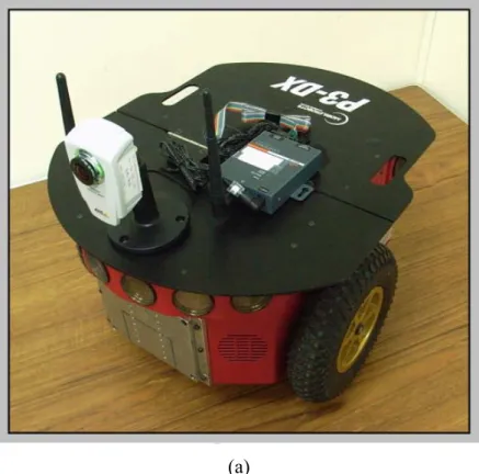
(20) Chapter 2 System Configuration and Navigation Principles. 2.1 Introduction For security surveillance, the utilization of a vision-based autonomous vehicle is good for saving manpower. The vehicle is dexterous, with its moving ability increasing the view range of security surveillance. Besides, it can also monitor lower or hidden objects that may be under a table or in a cabinet. In this study, two autonomous vehicles are used to perform the security patrolling task and each of them is equipped with a camera, as shown in Figure 2.1, though the proposed methods are general for any number of vehicles. Because the autonomous vehicles suffer from accumulation of mechanical errors, two cameras with fish-eye lenses, called top-view omni-cameras in the sequel, are installed on the ceiling. By the two cameras, autonomous vehicles can be located and controlled to navigate along correct paths. Between all on-board equipments and the user, some control and communication tools are required. The entire system configuration including hardware equipment and software are described in Section 2.2. Before all autonomous vehicles carry out the security patrolling task, a learning stage is necessary, in which the vehicles are taught where to go, what to do, and how to avoid collision with walls. The process to obtain all information that makes autonomous vehicles be able to accomplish the task assignment is described in 10.

(21) Section 2.3. The phase in which autonomous vehicles carry out security patrolling is called the navigation phase in this study. In Section 2.4, we will describe the vehicle guidance principle and the process of performing the monitoring task in the navigation phase.. (a) Figure 2.1 The vehicle used in this study is equipped with a camera. (a) A perspective view of the vehicle. (b) A front view of the vehicle. (c) A side view of the vehicle.. 11.

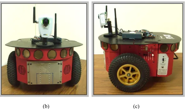
(22) (b). (c). Figure 2.1 The vehicle used in this study is equipped with a camera. (a) A perspective view of the vehicle. (b) A front view of the vehicle. (c) A side view of the vehicle. (continued). 2.2 System Configuration In this study, the vehicle system used as a test bed is composed of a Pioneer 3-DX vehicle made by MobileRobots Inc., a WiBox made by Lantronix, and an Axis 207MW camera made by AXIS, as shown in Figure 2.2. The Axis 207MW camera, called the camera system, not only is one part of the vehicle system but also plays an important role of monitoring and locating vehicles. Because the whole system, called the control system, is controlled by users remotely, some wireless communication equipment is necessary. All the details of the above equipments are described in Section 2.2.1. In order to develop the desired security surveillance system, we also need software that provides some commands and control interfaces. Besides, we also 12.

(23) provide an interface for users to control the vehicles and cameras. All the above utilities are described in Section 2.2.2.. (a). (b). (c). Figure 2.2 The vehicle system used in this study. (a) A Pioneer 3-DX vehicle. (b) A WiBox. (c) An Axis 207MW camera.. 13.

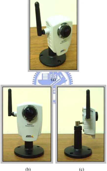
(24) 2.2.1. Hardware configuration. The entire structure of the vehicle system used in this study is shown in Figure 2.3. There are three principal parts: vehicle system, camera system, and control system. In the vehicle system, the Pioneer 3-DX vehicle is a 44cm×38cm×22cm aluminum body with two 19cm wheels and a caster. It can reach a speed of 1.6 meters per second on flat floors, and climb grades of 25o and sills of 2.5cm. At slower speeds it can carry payloads up to 23 kg. The payloads include additional batteries and all accessories. By three 12V rechargeable lead-acid batteries, the vehicle can run 18-24 hours if the batteries are fully charged initially. A control system embedded in the vehicle makes the user’s commands able to control the vehicle to move forward or backward or to turn around. The system can also return some status parameters of the vehicle to the user. To show the advantage of the mobile vehicle, a wireless connection between a user and the vehicle is necessary. A WiBox is used to communicate with the vehicle by RS-232, so the user has the ability of remotely controlling the vehicle over a network from anywhere. In the camera system, an Axis 207MW camera has the dimension of 85×55×40mm (3.3”×2.2”×1.6”), not including the antenna, and the weight of 190g (0.42 lb), not including the power supply, as shown in Figure 2.4. The maximum resolution of images is up to 1280×1024 pixels. In our experiment, the resolution of 320×240 pixels is used by the camera fixed on the vehicle and that of 640×480 pixels is used by the one fixed on the ceiling. Both of their frame rates are up to 15 fps. By wireless networks (IEEE 802.11b and 802.11g), captured images can be transmitted to users at speeds up to 54 Mbit/s. Each camera used in this study is equipped with a 14.

(25) fish-eye lens that will expend the field of view. Axis 207MW Camera. Computer. Control System. Camera System Access Point. Axis 207MW Camera. WiBox. Pioneer 3-DX Vehicle. Camera System Fixed on. RS-232. Vehicle System. Figure 2.3 Structure of proposed system. In the control system, a notebook PC is used to integrate the entire security patrolling system. With access points, all status information from vehicles and 15.

(26) cameras can be delivered to the user by wireless networks. The PC produces some commands according to these data. By the same way, vehicles can receive the commands from the control system and perform corresponding actions. In other words, an access point is a communication medium among the three systems.. (a). (b). (c). Figure 2.4 The camera system used in this study. (a) A perspective view of the camera. (b) A front view of the camera. (c) A left-side view of the camera.. 16.

(27) 2.2.2. Software configuration. ARIA (Advanced Robotics Interface Application) provided by MobileRobots, Inc. is an API (application programming interface) that assists developers in communicating with the embedded system of the vehicle, either using a serial or TCP/IP connection. It is a powerful object-oriented toolkit and usable under Linux or Win32 OS in C++. Therefore, we use the Borland C++ builder as the development tool in our experiments to control the vehicles by ARIA. The lowest-level data and other information of the vehicle can also be retrieved easily by means of the ARIA interface. About Axis 207MW camera controlling, the AXIS Company also provides a development tool called AXIS Media Control SDK. Using the Media Control ActiveX component from SDK, we can preview the image of the camera’s view and capture the current image data. It is also convenient for users to use it to develop any function with the images grabbed from the camera as input.. 2.3 Learning Principle and Proposed Process Because the patrolling environment is unknown, a learning strategy is necessary. For the purpose of learning all knowledge that makes the vehicles accomplish the mission successfully, we develop a learning interface for users. The entire learning process is shown in Figure 2.5. In this study, data having to be recorded are camera-related, object-related, and 17.

(28) area-related ones. The camera-related data are obtained from a camera calibration process. In this study, we don’t use the traditional camera calibration method to find a projective matrix for coordinate transformation. Instead, some landmarks on a pattern are utilized to acquire corresponding points between 2-D image and 3-D global spaces. For the camera fixed to ceilings in this system, the pattern is just the patrolling floor and the landmarks on it are just the corners of rectangular-shaped tiles. A user points some landmarks in the image by the user interface with a mouse, and corresponding points in the global space are calculated. Because each camera, used in our system, is equipped with a fish-eye lens, images captured by them are warped. Therefore, we use a bilinear interpolation method to translate coordinates in images into global space by these corresponding points. The object-related data are used to teach vehicles where to go and which direction to face when they perform the patrolling task. We drive a vehicle to the position where the vehicle can observe the monitored object and then record it as a monitoring point (MP) according to the image of a top-view omni-camera. For the purpose of learning the direction with respect to the object, we control the vehicle to face the object and let it move forward for a short distance. By the two positions of the vehicle (nodes), the direction angle can be obtained. The area-related data are about the environment where the vehicles patrol. An assumption made in this system is that the floor shape of the environment is composed of rectangular regions. At first, a user must key in corners in the clockwise order manually, and then all rectangular regions will be obtained. There might exist some pairs of MPs not belonging to an identical rectangular region, between which a vehicle cannot move straightly. Therefore, some points, called turning points, are necessary and they can be obtained by processing all the rectangular regions. With these turning points, the distances of all pairs of MPs can be calculated and which 18.

(29) turning points between two MPs are passed by can also be recorded. Start of Learning. Pointing Landmarks. Calculating Curve Lines and Intersections Corresponding Points between 2-D and 3-D. Driving Vehicle to Face Monitored Objects. Corners of Patrolling Area. Calculating Rectangle Regions. Localizing Vehicles. Rectangle Regions. Learning Vehicle Poses Calculating Turning Points. Vehicle Poses. Turning Points Calculating Distances between Monitored Points Distances and Paths between Monitored Points. Camera Calibration. Patrolling Area. Monitored Objects Learning Data. Navigation Information. Saving Data into Storage. End of Learning. Figure 2.5 Flowchart of proposed learning process. After all the data are obtained, they are saved into some text files. These files are then used in the navigation phase more than once.. 19.

(30) 2.4 Vehicle Guidance Principle and Proposed Process When the learning job has been done, all vehicles can start to perform the security patrolling task. The entire guidance process proposed in this study is shown in Figure 2.6. At first, the system reads all files that are obtained from the learning phase and contain information about the environment, autonomous vehicles, and monitored objects. According to the distances between all pairs of MPs, this system then plans random paths for each autonomous vehicle. If all differences between the paths of two vehicles do not exceed a threshold value which ensures the loads of all autonomous vehicles being balanced, the security patrolling task can be carried out. Because autonomous vehicles suffer from accumulation of mechanical errors, we need to locate them constantly. When a vehicle runs a fixed length of distance, it must be located by the top-view omni-cameras. By the values of the vehicles’ odometers, this system calculates the centroid of each vehicle from an image captured by a top-view omni-camera. The other function of the camera is to monitor vehicles to see whether they are still under control. If any vehicle loses control of its action, the system will stop all vehicles and send an alarm message to the user. Otherwise, the odometer of the vehicle is corrected and then the vehicle proceeds to move to its goal node. While the vehicles are carrying out the security patrolling, there could be collisions between vehicles. Therefore, the detection of collisions is necessary. This system computes the distance between two vehicles in every cycle of a fixed time duration and determines if they are too close. If true, the paths of the vehicles will be 20.

(31) changed. Start Security Patrol. Collision Avoidance. No Run a Timer. Detect Collision. Patrolling Paths. Read Files. Yes. Plan Paths for Vehicles No. Change Path. Conform Rules. Yes. Yes. Vehicle Localization. Move a Distance to Goal. Monitored Tasks No. No Calculate Vehicle Position in Image. Arrive Monitored Point Yes. Find Vehicle. Yes. Localize Vehicle Pose. Adjust Vehicle Direction. Patrol all Monitored Points. Image of Monitored Object. Image Database. No Stop all Vehicles and Send Alarm Message. Figure 2.6 Flowchart of proposed navigation process. A mission for the autonomous vehicles in this system is to take pictures of all the monitored objects during the navigation process. As a vehicle goes to a MP, it means that the vehicle will be in front of a monitored object. Therefore, the direction of the vehicle must be adjusted to face the object. Then the camera equipped on the vehicle takes a picture at the moment. The picture is transmitted to the control system by the wireless network and saved into an image file. When all the vehicles have accomplished their own patrolling paths, one cycle of security patrolling is finished. Then, the system will plan another set of new random paths for all the autonomous vehicles again. 21.

(32) Chapter 3 Learning Strategies for Navigation by Semi-automatic Driving. 3.1 Ideas of Proposed Techniques Used in Learning In this study, two cameras with fish-eye lenses fixed on ceilings are utilized to locate and monitor all autonomous vehicles. Before the use of the cameras, they must be calibrated. For this purpose, we propose in this study a point-correspondence technique integrated with an image interpolation method without conducting the conventional task of calculating the projection matrix for transforming points between 2-D image and 3-D global spaces. At first, by a mouse a user points out some landmarks in an image of a calibration target which is selected to be the tile pattern on the floor of our experimental environment. The landmarks we use in this study are the crossing points of the grid formed by the tile pattern. Such crossing points for use as corresponding points are abundant which yield better calibration accuracy in the proposed point-correspondence technique for camera calibration. The detail is described in Section 3.2. In an environment where autonomous vehicles navigate, it is indispensable to use some turning points in the navigation path to ensure no collision between the vehicles and the walls. To compute the turning points, the corner points of the walkable area are first utilized to acquire all rectangular regions within the entire area. Each region 22.

(33) is then represented by its upper-left and lower-right points. With these points, the system can judge whether the vehicles can move straightly between any pair of nodes where the vehicles visit (including the turning points). If two nodes belong to different regions, the vehicle will be guided to pass some turning points. In other words, the turning point is a medium that enables the vehicles to navigate between any pair of nodes without incurring collisions with the walls. Therefore, a turning point is selected to be the intersection of the centerlines of two overlapping regions or the center of the overlapping boundary of two adjacent ones. The details of the proposed techniques about processing rectangular regions and computing turning points are described in Section 3.3.1. Additionally, to take the pictures of monitored objects by cameras equipped on the autonomous vehicles, all nodes and directions with respect to the objects must be recorded. In this study, a learning technique is proposed to guide vision-based vehicles to capture pictures at suitable spots and directions. Two top-view omni-cameras are used. The process is described in detail in Section 3.3.2.. 3.2 Calibration of Top-View Omni-Cameras with Fish-Eye Lenses Each camera used in this study is equipped with a fish-eye lens. All images captured by the camera are warped. So the traditional camera calibration method of obtaining a global-space point via a projection-based transformation cannot be utilized directly; the cameras must be calibrated by another method, as mentioned 23.

(34) previously. For this, we propose a point-correspondence technique integrated with an image interpolation method. By the way, it is noted that the correct coordinates in the global space can be obtained from a warped image directly, as done in this study.. 3.2.1 Review of Conventional Camera Calibration Technique In general, a projection matrix is utilized in conventional methods to do the job of camera calibration. There are two kinds of parameters in the matrix, which must be calibrated, namely, the intrinsic and the extrinsic parameters. The intrinsic parameters do not depend on the position and orientation of a camera in the global space and include the focal length f, the image center point (u0, v0), the aspect ratio (Sx, Sy), and the skew error θs of the camera. Because the coordinate system of a camera and the global space may not be the same, the extrinsic parameters related to the rotation angle θ and the translation vector (t x , t y , t z ) of the camera must be calibrated. Based on the intrinsic and extrinsic parameters, the relation between points in 2-D image and 3-D global spaces may be described by Eq. (3.1) below [23], where the point (u, v)T is in the image coordinate system and the point (x, y, z)T is in the. global coordinate system:. 24.

(35) ⎛ x⎞ ⎛ u ⎞ ⎛ transformation ⎞ ⎛ transformation ⎞⎜ ⎟ ⎜ ⎟ ⎜ ⎟⎜ ⎟⎜ y ⎟ v = matrix of matrix of ⎜ ⎟ ⎜ ⎟⎜ ⎟ ⎜ 1 ⎟ ⎜ intrinsic parameters ⎟ ⎜ extrinsic parameters ⎟ ⎜ z ⎟ ⎝ ⎠ ⎝ ⎠⎝ ⎠ ⎜⎜ ⎟⎟ ⎝1⎠ ⎛ cos θ − sin θ 0 t x ⎞ ⎛ x ⎞ ⎛ S x f − S x f cot θ s u0 0 ⎞ ⎜ ⎟⎜ ⎟ ⎜ ⎟ ⎜ sin θ cos θ 0 t y ⎟ ⎜ y ⎟ . ≡⎜ 0 S y f / sin θ s v0 0 ⎟ ⎜ 0 0 1 tz ⎟ ⎜ z ⎟ ⎜ 0 ⎟ 0 1 0 ⎠ ⎜⎜ ⎟⎜ ⎟ ⎝ 0 0 0 ⎟⎠ ⎜⎝ 1 ⎟⎠ ⎝ 0. 3.2.2. (3.1). Proposed Calibration Technique. In the proposed calibration technique, we divide the patrolling area on the floor of the environment into multiple grids at first and all corners of them are called reference points. These points are the crossing points of the boundaries of the rectangular-shaped tiles on the floor. For every reference point, both of its coordinates in an image and in the global space must be recorded, describing a pair of corresponding points between the image and the global spaces. In order to acquire more corresponding points faster, we calculate all quadratic curves in the image of the patrolling floor area, of which the intersections are exactly the desired reference points. Note that because the images are captured by the cameras equipped with fish-eye lenses, a straight line in the global space appears as a quadratic curve in the image. Therefore, the technique is feasible. A quadratic curve can be calculated by three points at least. This property is utilized to find all curves. More specifically, we use a minimum mean-square-error (MMSE) method to calculate all the curves. Assume that a curve L is to be computed, which includes three parameters a, b, c. If points (x1, y1), (x2, y2), ..., (xn, yn) belong to the curve L, we JK K may acquire n curves which can be represented as a matrix in the form of Aw = b , as 25.

(36) shown in Eq. (3.2) below: L : y = a + bx + cx 2 , ( x1 , y1 ), ( x2 , y2 ), ..., ( xn , yn ) ∈ L JK K ⇒ Aw = b ⎡1 x1 ⎢ 1 x2 where A = ⎢ ⎢# # ⎢ ⎣⎢1 xn. x12 ⎤ ⎡ y1 ⎤ ⎡a ⎤ G ⎢ ⎥ 2 ⎥ JG y x2 ⎥ , w = ⎢⎢ b ⎥⎥ , b = ⎢ 2 ⎥ . ⎢#⎥ #⎥ ⎢⎣ c ⎥⎦ ⎢ ⎥ 2⎥ xn ⎦⎥ ⎣ yn ⎦. (3.2). JK The vector w can be computed by the MMSE criterion, that is,. JK K JK J ( w) = E[| b - Aw |2 ]; JK wˆ = arg min JG J ( w).. (3.3). w. Through a series of simplifications from Eq. (3.3), we can acquire a result as K ( AT A) wˆ = AT b .. (3.4). If all x1 , x2 , ..., xn are not equal, the matrix AT A is invertible and Eq. (3.4) can be solved to be: K wˆ = ( AT A)-1 AT b.. (3.5). Therefore, the curve L may be computed to be L : y = a + bx + cx 2 = [1 x. x 2 ]wˆ .. (3.6). Before calculating a curve, a user has to input the index of the curve and indicate that the curve is horizontal or vertical. As a curve is obtained, the pixels passed by the curve must record the index of the curve. The process of acquiring all quadratic curves is described as Algorithm 3.1 below. An example is shown in Figure 3.1 which is a result of acquiring some horizontal and vertical quadratic curves by the algorithm and each curve is calculated by four points on it. 26.

(37) Algorithm 3.1 Calculating a quadratic curve.. Input: An image I, the number n of points needed to calculate a curve, the index k of the curve, and being horizontal or vertical for the curve. Output: Pixels passed by the quadratic curve. Steps: Step 1.. Point out n points on the curve in the image I.. Step 2.. Calculate the curve by the MMSE criterion as described previously.. Step 3.. Record index k and the property of being horizontal or vertical into the table of pixels passed by the curve.. Figure 3.1 Calculating quadratic curves. When all curves are obtained, we check all pixels in the image. If a pixel is passed both by a vertical curve and by a horizontal one, the pixel is taken to be one of the reference points. The width and height of a grid in the global space are also taken as input by the user. According to the lengths and the total numbers of horizontal and vertical curves, the coordinates of all reference points in the global space can be 27.

(38) obtained. The entire process of acquiring all corresponding points between the image and global spaces is described as Algorithm 3.2 below. A result of finding all corresponding points from the image of one top-view omni-camera is shown in Figure 3.2.. Algorithm 3.2 Acquiring corresponding points between 2-D image and 3-D global. spaces. Input: An image I, the total number nx of vertical curves, the total number ny of horizontal curves, and the width w and height h of a grid in the global space. Output: The coordinates of all corresponding points. Steps: Step 1.. Repeat Algorithm 3.1 until enough curves are obtained.. Step 2.. Find all intersections from the result of Step 1 and record their coordinates in the image coordinate system.. Step 3.. Calculate all coordinates, with respect to the intersections obtained from Step 2, in the global coordinate system according to nx, ny, w and h, and then record them.. 28.

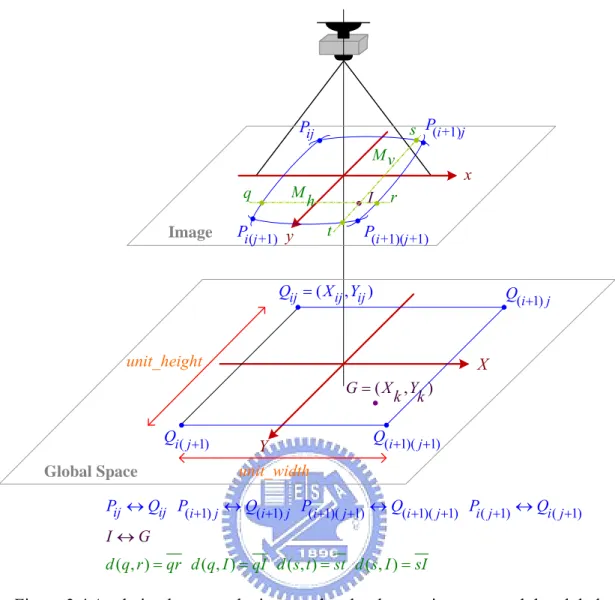
(39) Figure 3.2 Finding all corresponding points.. With the corresponding points, a bilinear interpolation method is used in this study to obtain the global-space coordinates with respect to the points in the warped image. Some assumptions involved are shown in Figure 3.3. The points Pij , P(i +1) j , P(i +1)( j +1) , Pi ( j +1) are the corners of the grid which point I belongs to. The lines L0, L1, L2 and L3 are straight lines through these corners. Mh is the line passing through point I and its slope is the mean of those of line L1 and line L3. Mv is the line passing through point I and its slope is the mean of those of line L0 and line L2. The points q and r are the intersections of Mh with L0 and L2, respectively. The points s and t are the intersections of Mv with L1 and L3, respectively.. 29.

(40) s. P(i+1)j. Pij L1 Mh. q. r I Mv. L0. Pi(j+1). L3. t. L2. P(i+1)(j+1). Figure 3.3 Point I in a distortion image. For a point in a warped image, we must judge which grid the point belongs to and calculate Mh, Mv, q, r, s and t. The ratios of distances are utilized to obtain the global-space coordinates with respect to the point. The equation is Eq. (3.7) below: d ( q, I ) d ( q, r ) d ( s, I ) Yk = Yij + unit _ height × . d ( s, t ). X k = X ij + unit _ width ×. (3.7). The points G ( X k , Yk ) and Qij ( X ij , Yij ) are in the global space with respect to point I and point Pij , respectively. The lengths unit_width and unit_height are the widths and the heights of a grid in the global space, respectively. The distance. d (q, I ) is the length from point q to point I. A graphic illustration is shown in Figure 3.4 and the process of acquiring the coordinates in the global space is described as Algorithm 3.3.. 30.

(41) s P(i +1)j. Pij Mv. q Image. M. t. Pi (j +1) y. r. I. h. x. P(i +1)(j +1). Qij = ( X ij , Yij ). unit_height. Q(i +1) j. X G = ( X ,Y ) k k. Qi ( j +1). Global Space. Y unit_width. Q(i +1)( j +1). Pij ↔ Qij P(i +1) j ↔ Q(i +1) j P(i +1)( j +1) ↔ Q(i +1)( j +1) Pi ( j +1) ↔ Qi ( j +1) I ↔G d (q, r ) = qr d (q, I ) = qI d ( s, t ) = st d ( s, I ) = sI. Figure 3.4 A relation between the image taken by the omni-camera and the global space.. Algorithm 3.3 Computation of coordinates in the global space.. Input: A point I in a warped image, the coordinates of all corresponding points, the width unit_width and the height unit_height of a grid in the global space. Output: The coordinates of the point G in global space with respect to the point I. Steps: Step 1.. Judge which grid point I belongs to.. Step 2.. Calculate lines L0, L1, L2 and L3 that are the straight lines through the corners of the grid to which point I belongs, as illustrated by Figure 3.3. 31.

(42) Step 3.. Calculate line Mh that passes through point I with its slope being the mean of those of line L1 and line L3.. Step 4.. Calculate line Mv that passes through point I with its slope being the mean of those of line L0 and line L2. Step 5.. Calculate points q and r that are the intersections of line Mh and the edges of the grid.. Step 6.. Calculate points s and t that are the intersections of line Mv and the edges of the grid.. Step 7.. Calculate point G ( X k , Yk ) by the following equation: d ( q, I ) ; d ( q, r ) d ( s, I ) Yk = Yij + unit _ height × . d ( s, t ) X k = X ij + unit _ width ×. Annotate that point Qij ( X ij , Yij ) is in the global space with respect to point Pij in the warped image.. 3.3 Information for Security Patrolling. 3.3.1 Proposed techniques of learning patrolling environment Information about the patrolling environment includes rectangular regions, which the floor shape is composed of, and the turning points among the regions. To find all rectangular regions, a user must key in all the corners of the patrolling area in the clockwise order. Because each point in the area belongs to one rectangular region at 32.

(43) least, a vertical line, called scanning line, is utilized to check whether some points in the vertical line do not belong to one region at least. If yes, another new rectangular region will be found for the points. The entire process and details are described as Algorithm 3.4 below.. Algorithm 3.4 Finding all rectangular regions.. Input: All corners of the patrolling area. Output: All rectangular regions of the patrolling area. Steps: Step 1.. Set a vertical line L through the leftmost corner of the patrolling area and scan the area from left to right.. Step 2. Find the intersections of L and the boundaries of the area, and record them. Record the corners of the boundary merely, if there is an overlap between L and the boundary. See the example shown in the following, where points a, b and c recorded.. Figure 3.5 Intersections of L and the boundaries of the area. Step 3. Divide these intersections into groups from top to down with each group including two points.. 33.

(44) See the example of Step 2 above for an illustration, where two groups (a, b) and (b, c) are obtained. Step 4. Judge where to set a line segment l. Step 4.1. Check whether the right part of a group is the inner range of the patrolling area and a rectangular region in the range has not been found. If yes, go to Step 4.2; else, continue to check the next group. Annotate that the technique of checking whether the right part of a group is the inner range of the patrolling area is described in Algorithm 3.5. Step 4.2. Set l in the following way. Step 4.2.1. Shift the middle point M of the group one pixel to the right. Step 4.2.2. Extend M along a vertical direction until colliding with the boundaries, where the line l is set. See the example shown in the following, where line de is l mentioned above. a. d. Region1 b M =(. c. a+b ) 2. e. Figure 3.6 Setting a line segment l. Step 5. Continue scanning the line segment l to the left until colliding with the boundary of the patrolling area. See the example shown in the following.. 34.

(45) Region1. scanning l. Figure 3.7 Scanning the line segment l to the left. Step 6. Continue scanning the line segment l to the right until colliding with the boundary of the patrolling area. See the example shown in Step 5, where Region2 was obtained.. Region1. scanning. Region2. l. Figure 3.8 Scanning the line segment l to the right. Step 7. Continue scanning the vertical line L to the right and repeat Step 2 until L reaches the rightmost boundary of the patrolling area.. Algorithm 3.5 Judging an inner range.. Input: All corners C of the patrolling area, and two points P whose x-coordinates are 35.

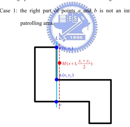
(46) the same. Output: An indication whether the right part of P is an inner range of the patrolling area. Steps: Step1. Calculate the middle point M of the two points P. Step2. Shift M one pixel to the right. Step3. Set a vertical line LM through point M. Step4. Check the numbers of intersections of the line LM and the boundary. If both the number of the upper part and that of the lower one of M are odd and either part does not include an overlapping line, it is decided that the right part of P is an inner range of the patrolling area. See the graphic illustration shown in the following. Case 1: the right part of points a and b is not an inner range of the patrolling area. L a (x, y1 ) M ( x + 1,. y1 + y2 ) 2. b (x, y2 ). c. Figure 3.9 The right part of points a and b is not an inner range.. Case 2: the right part of points b and c is an inner range of the patrolling area.. 36.

(47) L a. b (x, y1 ) M ( x + 1,. y1 + y2 ) 2. c (x, y2 ). Figure 3.10 The right part of points a and b is an inner range.. Now, we show a result of Algorithm 3.4. A patrolling area is shown in Figure 3.11. The total number of rectangular regions in the patrolling area is seven and they are shown in Figure 3.12 through Figure 3.18 step by step.. Figure 3.11 A patrolling area. According to these rectangular regions, we can compute all desired turning points. If two regions are overlapping or adjacent, we can obtain a turning point. The point is the intersection of two vertical and horizontal centerlines of the regions. The process of finding all turning points is described as Algorithm 3.6 and the result in the patrolling area of Figure 3.11 is shown in Figure 3.19. The eight circles in Figure 3.19 are exactly the turning points, in which each blue one is the center of the overlapping 37.

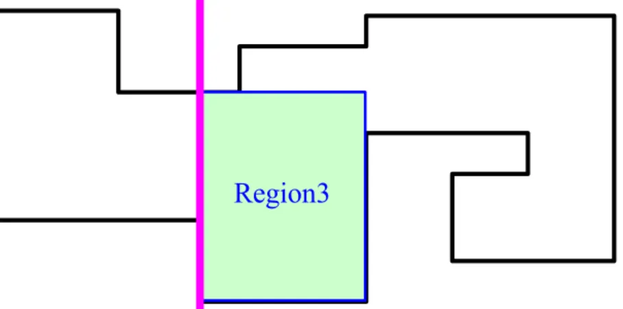
(48) boundary of two adjacent regions.. Region1. Figure 3.12 The first rectangular region.. Region2. Figure 3.13 The second rectangular region.. Region3. Figure 3.14 The third rectangular region. 38.

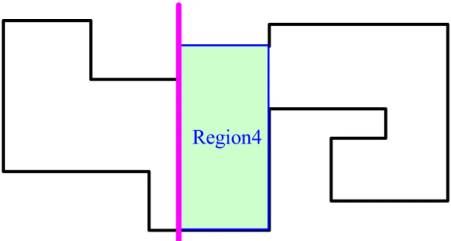
(49) Region4. Figure 3.15 The fourth rectangular region.. Region5. Figure 3.16 The fifth rectangular region.. Region6. Figure 3.17 The sixth rectangular region.. 39.

(50) Region7. Figure 3.18 The seventh rectangular region.. Algorithm 3.6 Finding all turning points.. Input: All rectangular regions R in an area. Output: All turning points. Steps: Step1.. Take a pair of overlapping or adjacent regions from the set R. If the two regions are overlapping, go to Step2; else, go to Step4.. Step2.. Calculate all vertical and horizontal centerlines of the two regions.. Step3.. Find an intersection within these centerlines, which is exactly a turning point of the area.. Step4.. Calculate the center of overlapping boundary, which is exactly a turning point of the area.. Step5.. Repeat Step 1 until all regions in R have been checked.. 40.

(51) Figure 3.19 All turning points in the area.. 3.3.2 Learning of poses of vehicles with respect to monitored objects To learn the poses of autonomous vehicles with respect to monitored objects, we designed a user interface, as shown in Figure 3.20. The image in the interface is the real-time view of the camera installed on an autonomous vehicle. Before learning, a vehicle is parked at the origin of the global space. Because the vehicle suffers from mechanic errors, a user must constantly locate it by the top-view omni-cameras in the period of the learning phase. We can use a joystick or the buttons in the user interface to control the moves of the vehicle. As the vehicle has moved a short distance, the user must press the “Localize” button in the interface. For an example, Figure 3.21 shows a situation that the vehicle is ready to be located. After the user presses the “Localize” button, the system will calculate the centroid of the vehicle in the image captured by a top-view omni-camera. Then, the centroid is transformed from the image space into the global space and the odometer value of the 41.

(52) vehicle is corrected by the coordinates of the resulting point.. Figure 3.20 User interface of learning MPs.. Figure 3.21 Before localizing the vehicle. In Figure 3.22, the green component is the vehicle and a white circle in the component is its centroid. The entire detail of the technique is described in Section 4.2.2. 42.

(53) For the direction with respect to monitored objects, we utilize two points to obtain the direction vector. First, we drive the vehicle to the front of a monitored object, leaving a sufficient distance between the vehicle and the object. At the moment, we adjust the orientation of the vehicle by the image in the user interface. As the monitored object appears at the center of the image, we locate the vehicle by pressing the “Localize” button. Furthermore, we move the vehicle forward a short distance and press the “Learn MP and Direction” button. For the example shown in Figure 3.23, the safe deposit labeled by a red rectangle is a monitored object and the vehicle faces the object. The detail process is described as Algorithm 3.7.. Figure 3.22 Localizing the vehicle.. 43.

(54) Figure 3.23 The vehicle in front of a monitored object.. Algorithm 3.7 Learning poses of vehicles with respect to monitored objects.. Input: The position P of the vehicle in front of a monitored object. Output: The pose of the vehicle with respect to the object. Steps: Step 1. Drive the vehicle to the position P. Step 2. Let the vehicle face the object. Step 3. Localize the vehicle. Step 4. Move the vehicle forward a short distance. Step 5. Localize the vehicle again and save its pose.. 44.

(55) Chapter 4 Security Patrolling by Multiple Vehicle Navigation. 4.1 Introduction to Concepts in Proposed Systems In the study, we use multiple vision-based autonomous vehicles to perform security patrolling. To obtain more benefits, there must be ideal path planning for all vehicles. By an optimal randomization technique proposed in this study and described in this chapter, these patrolling paths have the properties of randomization, optimization, and load balancing within all vehicles. Furthermore, two cameras with fish-eye lenses are utilized to localize and monitor all the vehicles. All concepts of the above are described in following five sections.. 4.1.1. Randomized patrolling. The patrolling path of every autonomous vehicle is produced to be random. Random paths are good for security surveillance. Because a fixed path will reveal where a vehicle is located at a fixed moment, thieves can, by such observation, invade and steal those valuable objects which are not guarded by any vehicle at the time. To randomize a patrolling path, all nodes (MPs) in the path with respect to monitored 45.

(56) objects are chosen randomly. Furthermore, if the time interval between two patrollings of a monitored object is smaller, the security of the objects will be raised. Therefore, each node (MP) is just chosen once in a patrolling session.. 4.1.2. Optimal path. After the nodes of a patrolling path are determined, the order of passing these nodes is computed. To decrease the time taken to accomplish security patrolling in one patrolling session, the distance of each path must be made to be the shortest. A method for this purpose by finding the Hamiltonian path is utilized and the detail of determining all patrolling paths is described in Chapter 5.. 4.1.3. Load balance. To obtain more benefits of using multiple autonomous vehicles to perform the security patrolling, the loads for all vehicles must be balanced. We set a threshold parameter to restrict the differences of the patrolling distances. After all patrolling paths are produced, we check whether the differences of these paths are acceptable according to the threshold; if not, the nodes of all paths must be chosen afresh.. 4.1.4. Top-view omni-monitoring. In this study, two cameras are fixed on the ceiling and each of them is equipped 46.

(57) with a fish-eye lens. That is the reason why the camera is called a top-view monitoring omni-camera. At times, there may be some unexpected problems with the vehicles, such as not complying with the user command. The cameras can overlook the patrolling area and so control all actions of the vehicles. If one vehicle is not under control, all vehicles will be stopped. And then the system will send an alarm message to the control center.. 4.1.5 Path correction by top-view monitoring omni-camera Autonomous vehicles used in this study are subject to accumulation of mechanic errors, so they must be localized periodically. About vehicle localizations, house corners, geometric shapes, and object features all may be utilized to localize the vehicle. For the vehicle localization technique proposed in this study, the top-view omni-cameras are utilized. Because the cameras are fixed, images acquired by them are good for analyzing the actual positions of the vehicles. The entire detail of vehicle localization is described in Section 4.2.2.. 47.

(58) 4.2 Proposed Techniques Used in Patrolling. 4.2.1 Optimal randomized patrolling paths for all vehicles All patrolling paths planned by algorithms proposed in this study have three properties: randomization, optimization, and load balancing. Let the total number of autonomous vehicles and monitoring positions (MPs) be nv and nm, respectively. In the proposed method for generating random patrolling paths, we divide all MPs into nv groups randomly. Assume that the number of chosen MPs for the i-th vehicle is ni, so that the numbers can be represented as (n1, n2, ..., nnv). Each ni must satisfy two conditions as listed in the following. Condition 1: n1 + n2 + ...+ nnv = nm − nv Condition 2: ⎢ nm − nv ⎥ ⎡ nm − nv ⎤ ⎢ ⎥ − Tvalue ≤ ni ≤ ⎢ ⎥ + Tvalue, i = 1, 2, ..., nv n n v v ⎣ ⎦ ⎢ ⎥. where Tvalue is an adjustable parameter. Because nv MPs are patrolled by nv vehicles at the end of the t-th session, there is no need to visit the nv MPs again in the (t + 1)-th session. That is the reason why “nm − nv” is included in Condition 1. Additionally, the purpose of Condition 2 is to achieve load balancing among all vehicles. Because we set a threshold parameter T to restrict the differences of the patrolling distances, each 48.

(59) ⎢n − n ⎥ ⎡n − n ⎤ ni dose not have to be equal to the mean ⎢ m v ⎥ or ⎢ m v ⎥ . Therefore, we add ⎣ nv ⎦ ⎢ nv ⎥ ⎡n − n ⎤ the parameter Tvalue to obtain an upper bound “ ⎢ m v ⎥ +Tvalue” and a lower ⎢ nv ⎥ ⎢n − n ⎥ bound “ ⎢ m v ⎥ − Tvalue ” for all ni. The parameters Tvalue and T are adjustable. If ⎣ nv ⎦. they are smaller, the time taken to determine all patrolling paths is larger, but the loads of all vehicles will be more balanced. The state of choosing MPs for all vehicles can be represented as n − nv − n1 − n2 −...− nnv −1. ( Cnn1m − nv , Cnn2m − nv − n1 ,..., Cnnvm. ).. The combination Ckn is the number of picking k MPs from n MPs randomly, defined as. ⎛n⎞ n! Ckn ≡ ⎜ ⎟ ≡ . ⎝ k ⎠ k !(n - k )!. (4.1). For example, assume that the number of MPs is “thirteen”, the number of vehicles is “three”, and the parameter Tvalue is “one”. By Condition 1, “ten MPs” need be divided into “three groups.” Besides, the number of each group has an upper bound of “five” and a lower bound of “two” by Condition 2. The three states of the numbers of MPs chosen for three vehicles are shown in following. (1) (5,3,2) (2) (4,4,2) (3) (4,3,3) For state (1), the number of the combination is C510 ∗ C35 * C22 =2520. For state (2), the. 49.