Simultaneous Synthesis of Flexible Heat-Exchange Networks with
Uncertain Source-Stream Temperatures and Flow Rates
Cheng-Liang Chen* and Ping-Sung Hung
Department of Chemical Engineering, National Taiwan University, Taipei 10617, Taiwan, ROC
In this paper, a novel strategy for the synthesis of cost-effective flexible heat-exchange networks (HENs) that involves specified uncertainties in the source-stream temperatures and flow rates is presented. The problem is decomposed into three main iterative steps: (1) simultaneous HEN synthesis to attain a network configuration with a minimum total annual cost (TAC); (2) flexibility analysis to test whether the network obtained from the synthesis step is feasible in the full disturbance range; and (3) integer cuts to exclude disqualified network configurations, i.e., for those networks not passing the examination of the flexibility analysis, the integer cuts and/or some parameter points will be appended to narrow the search space used for further HEN synthesis. A few iterations of these three steps are required to secure the desirable results. In addition to the theoretical derivation, two examples are included to demonstrate the efficiency of the proposed strategy.
1. Introduction
As complicated as it is, a standard heat-exchange network (HEN) synthesis problem can be stated as follows: Given hot/cold process streams to be cooled/ heated from nominal supply temperatures to specified target temperatures and heating/cooling utilities, syn-thesize an HEN configuration to reach some assigned objective(s) such as the minimum utility consumption, the minimum total number of heat-exchange units, the minimum total exchanger area, the minimum total annual cost (TAC), etc. HEN synthesis is by far one of the most developed fields for which many techniques, such as evolutionary design methods (e.g., pinch design method1) or mathematical programming approaches
(e.g., sequential2or simultaneous optimization3,4), have
been proposed.5A review with an annotated
bibliogra-phy on HEN synthesis methods proposed in the 20th century can be found in the recent literature;6therein,
a timeline of innovation and major discoveries in HEN synthesis are also addressed.
Such issues as utility consumption, matching num-bers, and total area for HEN synthesis and the capabil-ity of HENs for feasible operation under possible variations of source-stream temperatures and flow ratessthe typical design objectivesshave also been emphasized in some articles.7-12For example, Floudas
and Grossmann11proposed a novel sequential synthesis
method that combines the multiperiod mixed-integer linear programming (M-MILP) transshipment model, used for generating the set of stream matches; the nonlinear programming (NLP) formulation, used for synthesizing the multiperiod networks; and the active set strategy,10used for performing the flexibility
analy-sis over the full disturbance range at the levels of matches and structures. Illustrations show that a few iterations are usually required in the synthesis and flexibility analysis stages. However, the formulation and the synthesis procedure are somewhat tedious in treat-ing the partitiontreat-ing of temperature intervals under
uncertain inlet temperatures. Aaltola12proposed using
a multiperiod simultaneous mixed-integer nonlinear programming (MINLP) model for minimizing the total annual cost (TAC) and generating a flexible heat-exchange network directly. Not relying on a sequential decomposition, this method seems simple and straight-forward. However, the operational feasibility of the resulting network is not guaranteed because only a finite number of operating conditions are considered during the design.
In this paper, the authors try to take advantage of both approaches11,12for the synthesis of a flexible
heat-exchange network. In this novel approach, the flexible HEN synthesis problem is decomposed into three main iterative steps: simultaneous HEN synthesis for con-sidering a finite number of operating conditions, flex-ibility analysis for testing the feasflex-ibility of the network over the full disturbance ranges, and integer cuts for excluding the disqualified networks. In the simulta-neous synthesis step, the problem is formulated as a multiperiod mixed-integer nonlinear programming (MM-MINLP) for minimizing the TAC of the network based on the stagewise superstructure proposed by Yee and Grossmann.3,4In the flexibility analysis step, we solve
the flexibility index evaluation problem for the network structure obtained from the synthesis step by directly applying the active set strategy.10,11Should the resulting
network(s) not pass the flexibility test, the associated integer cuts would be appended to the search space to exclude the same network(s) from consideration. In addition, a set of additional extreme parameter points can also be included to reduce the feasible space and to accelerate the design process. To obtain the final quali-fied network configuration, several iterations of such network synthesis and flexibility analysis steps might be required. According to the results of simulations with examples modified from those of Floudas and Gross-mann,11 the efficiency of the proposed flexible HEN
synthesis method is quite satisfactory.
* To whom correspondence should be addressed. Tel.: 886-2-23636194. Fax: 886-2-23623040. E-mail: [email protected]
10.1021/ie030701f CCC: $27.50 © 2004 American Chemical Society Published on Web 07/23/2004
2. Problem Definition and Outline of the Proposed Flexible HEN Synthesis Strategy
An HEN synthesis problem with NHhot streams and NCcold streams along with possible variations in input
temperatures and heat capacity flow rates is considered here. Let θ denote the vector of uncertain parameters with the nominal value θ0. Suppose ∆θ-and ∆θ+are
the maximum expected deviations of these uncertain parameters in the negative and positive directions. The flexible HEN synthesis problem can then be defined as synthesizing a cost-effective heat-exchange network that is feasible for all possible operating points contained in P(δ ) 1),11where
As is pointed out in the literature,7,10,13this problem is
difficult to solve directly because it involves a max-min-max constraint. In other words, the feasible region defined by the inequality energy balance constraints is nonconvex,14 so the critical point that confines the
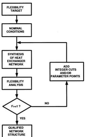
solution might not rest on the vertexes of the polyhedral region of uncertainty. It is this difficulty that motivates us to separate the flexible HEN design into iterative steps, as depicted in Figure 1. Except for the finite extreme operating conditions considered in the synthe-sis to narrow the search space, the desired ranges of operating flexibility, that is, the feasible ranges for uncertain source-stream temperatures and/or flow rates, should be assigned at first. Instead of directly including this flexibility target in the HEN synthesis, the allow-able operational range is evaluated and qualified for a candidate network structure. Those disqualified net-works are excluded by appending the integer cuts in the search space for subsequent network synthesis. The proposed strategy for the flexible HEN synthesis in-volves the following three main iterative steps:
1. Synthesis of a Multiperiod Network via Si-multaneous Optimization. According to the
super-structure-based multiperiod MINLP formulation for HEN synthesis discussed in section 3, a heat-exchange network can be synthesized by means of any existing mixed-integer nonlinear optimization algorithm. Several extreme operating periods can be considered simulta-neously to reduce the search space, although the num-ber of continuous variables is increased dramatically. The flexibility requirement is not directly taken into account in this synthesis step to simplify the calculation.
2. Evaluation of the Flexibility Index. In this
stage, the flexibility index of the network resulting from the previous synthesis step is evaluated to determine whether the current network satisfies the previously assigned flexibility target, that is, whether the network can be operated over the full range of possible input stream temperatures and flow rates. Here, the flexibility index is determined by using the active set strategy proposed by Grossmann and Floudas10and reviewed in
section 4 to take into account the possibility of nonex-treme critical points. If the current HEN structure meets the requirement of the flexibility target, it can be directly accepted as a qualified network to terminate the search. On the other hand, if the resulting flexibility index does not satisfy the target, then a new network structure with improved operational flexibility must be found by using the procedure listed in the following step.
3. Integer Cuts To Exclude the Disqualified Networks. For disqualified network structures, the
integer cuts expressed in eq 15 and/or some additional extreme points can be appended to the original structure to reduce the search space and then go back to the synthesis step for iteration to find a new candidate network.
Several iterations of these three steps are sometimes required to attain a qualified configuration. Neverthe-less, the proposed strategy is attractive enough because it prevents the necessity to include a large number of constraints and operating points directly in the formu-lation. To illustrate how to carry out the whole synthesis procedure, the authors present two examples in section 6. Through the numerical simulations, it can be verified that the proposed strategy is easy to implement and can provide a feasible and balanced solution for the heat-exchange network synthesis problem.
3. Synthesis of Multiperiod Heat-Exchange Networks
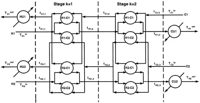
The stagewise superstructure proposed by Yee and Grossmann3,4is applied to construct the configuration
of a heat-exchange network, as it is suitable for formu-lating a simultaneous solution that involves the con-sideration of total utility consumption, the total number of matches, and the total area of heat-exchange units. A two-stage superstructure with two hot and two cold streams is shown in Figure 2 for reference; the mean-ings of relevant notations in the structure can be found in either Yee and Grossmann3,4or the Nomenclature
section.
Instead of directly considering all possible combina-tions of uncertain input temperatures and heat capacity flow rates for the flexible network synthesis, only a finite number of extreme operating conditions are taken into account for network design to reduce the search space. The mathematical programming formulation for mini-mizing the total annual cost, TAC, which includes the Figure 1. Proposed strategy for flexible HEN synthesis.
average costs of hot and cold utility consumption over a finite number of operating points and the annual costs of installation and material of the heat-exchange units, can be summarized as follows3,4,15
where x and Ω denote the design variables and the feasible search space comprising all material/energy balance constraints and relevant logical constraints, respectively. VT ) {0, 1, ..., NV} is the index set, in
which zero denotes the nominal conditions (or the base case), for numbering a limited number of extreme operating conditions used for finding the optimal final structure. These possible operating vertexes are applied here to help reduce the search space in the design stage.
Here, LMTDijkis the log-mean approaching temperature
for the matching of hot stream i and cold stream j at the kth stage. Chen’s approximation is used for LMT-Dijk.16 LMTDi,cu and LMTDhu,j are defined and
ap-proximated similarly.
Note that the inclusion of each of the extreme periods increases the total number of continuous variables; therefore, the designer should make a tradeoff between the number of variables and the search space. There are a total of 4NH+NC vertexes for an HEN synthesis
problem with NHhot and NCcold streams that can vary
in temperatures and flow rates. It is impractical to include simultaneously all of those operating extremes for resilient network design because of the dramatic increase of the number of continuous variables for each of these extreme situations. Marselle et al.7suggested
considering the states that tend to maximize the need for exchangers, coolers, and heaters, which are deter-mined as follows. The case of all streams with the maximum heat capacity flow rates and with the maxi-mum (minimaxi-mum) supply temperatures for all hot (cold) streams tends to result in a network configuration with the maximum heat-exchange area. The instance of the highest cooling requirement (i.e., all hot streams have the upper-bound temperatures and heat capacity flow rates) and the lowest cooling capability (all cold streams have the upper-bound temperatures and the lower-bound heat capacity flow rates) tends to be a network consuming the maximum cooling utility. A network in which the highest heating requirement for the cold streams (minimum temperatures and maximum flow rates) is paired with the lowest heating capability for hot streams (minimum temperatures and flow rates) needs the maximum heating utility. As pointed out by Marselle et al.,7a network that can handle these three
extreme periods does not necessarily imply that all states within the disturbance range can be operated adequately. Although a quantitative flexibility analysis is still relevant to clarify the feasible operating range of the network, the network combining these three extreme periods represents a highly resilient network candidate. Other vertexes are seldom applied for design in the literature except for problems considering uncer-tain supply temperatures only.17
4. Flexibility Analysis
The solution of eq 2 is a heat-exchange network with a minimum TAC under a specific configuration that satisfies multiple extreme operating conditions. When the resulting network is applied to a process with the consideration that the source-stream temperatures and heat capacity flow rates can vary in the full range of uncertainty, its flexibility can be measured by the flexibility index proposed by Swaney and Grossmann.9
To carry out the flexibility analysis, all relevant equality min x∈Ω TAC ) 1 NV+ 1 (
∑
∀n∈VT∀∑
i∈HP Ccuqcui(n)+∑
∀n∈VT∀∑
j∈CP Chuqhuj(n)) +∑
∀i∈HP∀∑
j∈CP∀∑
k∈ST Cij[
max ∀n∈VT(
qijk(n) UijLMTDijk(n))
]
(2) +∑
∀j∈CP Chu,j[
max ∀n∈VT(
qhuj (n) Uhu,jLMTDhu,j (n))
]
+∑
∀i∈HP Ci,cu[
max ∀n∈VT(
qcui(n) Ui,cuLMTDi,cu (n))
]
x≡{
zijk, zcui, zhuj; tik (n) , tjk (n) , ti,N(n)T+1, tj,N(n)T+1; dtijk (n) , dtij,N(n)T+1, dtcui (n) , dthuj (n) ; qijk (n) , qcui (n) , qhuj (n) ; ∀i∈ HP, j ∈ CP, k ∈ ST, n ∈ VT
}
(3) LMTDijk) (tik- tjk) - (ti,k+1- tj,k+1) ln tik- tjk ti,k+1- tj,k+1 (5) ≈[
(tik- tjk)(ti,k+1- tj,k+1)×(
tik+ ti,k+1 2 -tjk+ tj,k+1 2)
]
1/3and inequality constraints for the heat-exchange net-work model can be reorganized as described in eqs 6 and 7. It should be noted that the overall heat balances are not included because they can be obtained by combining other independent equalities.
The variables in these equations are classified into four categories. θ is the vector of uncertain parameters (i.e., temperatures and flow rates defined in eq 1). The design variables d, obtained from the synthesis step, define the network structure and the sizes of the heat-exchange units. The control variables u represent the degrees of freedom in the operation of the network. w, the state variables, can be expressed as implicit functions of control variables u and uncertain parameters θ by solving the independent equality constraints.
Thus, the inequalities of the network can be represented by the following equation, where CI is the index set of condensed inequalities
By rearranging the related equations, the flexibility index problem of a network can be formulated as the following mixed-integer nonlinear programming prob-lem10,11,15
In these equations, F represents the quality of flexibility level, where an F with value of less than 1 means that the network is not operable within the full range of definite uncertain parametric bounds; sm are slack
variables; λm are Kuhn-Tucker multipliers; ym ) 1
indicates active constraints; V is a sufficiently large real number; and nuis the number of control variables u.
Details of the above MINLP formulation can be found in the literature.10,11
The active set strategy, illustrated in eq 10 for solving the mixed-integer optimization problem, consists of three basic steps.10,11 First, the active candidate sets
Figure 2. Two-stage superstructure.
h(d,u,w,θ) )
{
∑
∀j∈CP qijk- (tik- ti,k+1)FCpi∑
∀i∈HP qijk- (tjk- tj,k+1)FCpj qcui- (ti,NT+1- Ti out )FCpi qhuj- (Tjout- tj1)FCpj Tiin- ti1 Tjin- tj,N T+1}
) 0 (6) g(d,u,w,θ) ){
ti,k+1- tik tj,k+1- tjk Ti out- t i,NT+1 tj1- Tjout ∆Tmin+ tjk- tik ∆Tmin+ tj,NT+1- ti,NT+1 ∆Tmin+ TCU out- t i,NT+1 ∆Tmin+ tj,1- THU out}
e 0 (7) h(d,u,w,θ) ) 0 f w ) w(d,u,θ) (8) gm[d,u,w(d,u,θ),θ] ) fm(d,u,θ) e 0 ∀m∈ CI (9) F ) min θ,u,sm,λm,ym,δ δ s.t. sm+ fm(d,u,θ) ) 0∑
∀m∈CI λm ∂fm ∂u ) 0∑
∀m∈CI λm ) 1 λm- ym e 0}
f (10) sm- V(1 - ym) e 0∑
∀m∈CI ym) nu+ 1 θ∈ P(δ), ym∈{0, 1} δ, λm, smg 0, ∀m∈ CIshould be identified. Let NAS){1, ..., nAS}denote the
index set of all possible combinations for the active constraints and AS(k) represent the kth index set of the active constraints. Then, a value of δkfor the kth active
candidate set can be obtained by solving the following nonlinear programming (NLP) problem11
The solution of the flexibility index problem is given by
Notice that, for problems in which there is no control variable (i.e., nu) 0), the flexibility analysis problems
are much simpler.10 In such a case, the stationary
conditions in eq 10, that is, the three relations marked with a f and the associated Kuhn-Tucker multipliers λm, can be eliminated. In this condensed formulation,
only one constraint is allowed to be active for each active set. Equation 10 can thus be decomposed in terms of each individual constraint, that is, AS(k) ){k}, ∀k∈ NAS. The flexibility index problem is therefore simplified
significantly.
5. Integer Cuts for Excluding the Disqualified Networks
If an HEN resulting from the previous formulation is not qualified in the flexibility test, a different HEN should be proposed as the new candidate. To avoid coming up with a same HEN structure that has been eliminated in the previous nRiterations, one should add
some constraints in the (nR+ 1)st synthesis formulation.
Herein, two kinds of networks are guaranteed to be brand-new: one that has at least one different unit from any earlier eliminated network and one that whose units are only part of those of any earlier eliminated network. These two conditions can be expressed by the following logic constraints for the (nR+ 1)st network
and
and
Here, z•l and nSNl denote the associated integer value
and the total number of selected units, respectively, of the l th eliminated network, l ) 1, ..., nR. Let a new
binary variable zdl denote the toggle switch of these two acceptable conditions, i.e., zdl ) 1 for case 1 and zdl ) 0 for case 2. Then, the above logic constraints can be expressed as
These two expressions can be further combined into a single integer cut equation. These integer cuts in the search space can guarantee that a network candidate different from all previously disqualified configurations is attained
6. Numerical Examples
Examples adapted from Floudas and Grossmann11are
used here to demonstrate the efficiency of the proposed strategy. To solved the MINLP for HEN models, the General Algebraic Modeling System (GAMS)18is used
as the main solution tool. The MINLP and NLP solvers are SBB and CONOPT3 for both examples.
Example 1. A Two-Hot/Two-Cold Streams Prob-lem. The first example involves two hot and two cold
streams (NH) 2, NC) 2) along with steam and cooling
water, respectively, as the heating and cooling utilities. The data for the problem, including the nominal operat-ing conditions as well as three periods of extreme operating conditions, are listed in Tables 1 and 2. Under δk) min θ,u,δ δ s.t. fm(d,u,θ) ) 0 θ∈ P(δ) (11) δ g 0 ∀m∈ AS(k) ⊆ CI F ) min ∀k∈NAS δk (12) Case 1
∑
∀i∈HP∀∑
j∈CP∀k∑
∈ST (1 - zijkl )zijk nR+1+∑
∀i∈HP (1 - zi,cul )zi,cu nR+1+∑
∀j∈CP (1 - zhu,jl )zhu,j nR+1 g 1∑
∀i∈HP∀∑
j∈CP∀k∑
∈ST zijk l zijk nR+1+∑
∀i∈HP zi,cu l zi,cu nR+1+∑
∀j∈CP zhu,jl zhu,jnR+1 e nSN l Case 2∑
∀i∈HP∀∑
j∈CP∀k∑
∈ST (1 - zijkl )zijk nR+1+∑
∀i∈HP (1 - zi,cul )zi,cu nR+1+∑
∀j∈CP (1 - zhu,jl )zhu,j nR+1 g 0Table 1. Cost Data for Example 1
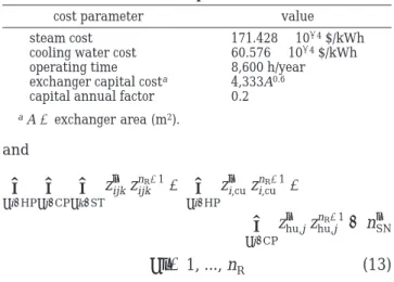
cost parameter value steam cost 171.428× 10⁻⁴$/kWh cooling water cost 60.576× 10⁻⁴$/kWh operating time 8,600 h/year exchanger capital costa 4,333A0.6
capital annual factor 0.2
aA ) exchanger area (m2).
∑
∀i∈HP∀∑
j∈CP∀∑
k∈ST zijkl zijknR+1+∑
∀i∈HP zi,cul zi,cunR+1+∑
∀j∈CP zhu,jl zhu,jnR+1< n SN l ∀l ) 1, ..., nR (13)∑
∀i∈HP∀∑
j∈CP∀∑
k∈ST (1 - zijkl )zijknR+1+∑
∀i∈HP (1 - zi,cul )zi,cunR+1+∑
∀j∈CP (1 - zhu,jl )zhu,jnR+1 g zd l∑
∀i∈HP∀∑
j∈CP∀∑
k∈ST zijkl zijk nR+1+∑
∀i∈HP zi,cul zi,cu nR+1+∑
∀j∈CP zhu,jl zhu,j nR+1 e nSNl - 1 + zdl zdl ∈{0, 1}, l ) 1, ..., nR (14) 2(∑
∀i∈HP∀∑
j∈CP∀∑
k∈ST zijkl zijknR+1+∑
∀i∈HP zi,cul zi,cunR+1+∑
∀j∈CP zhu,jl zhu,j nR+1) - (∑
∀i∈HP∀∑
j∈CP∀k∑
∈ST zijk nR+1+∑
∀i∈HP zi,cu nR+1+∑
∀j∈CP zhu,j nR+1 ) e nSNl - 1 l ) 1, ..., nR (15)the conditions that the expected maximum operating disturbances are (10 K for stream hot-1 and (5 K for stream cold-2 in temperature and (0.4 kW K-1for both streams hot-1 and cold-2 in heat capacity flow rate, the objective is to derive a heat-exchange network config-uration that is feasible for the specified disturbance range and features the minimum TAC. The minimum number of superstructure stages, NT, is set at 2 because
max{NH, NC} ) 2.3 The proposed iterative solution
strategy is illustrated in the following discussion. To show the effect of appending the extreme operating periods mentioned in section 3 and the integer cuts on the reduction of the search space, one extreme period and one integer cut per iteration are added to the model until a feasible solution is achieved.
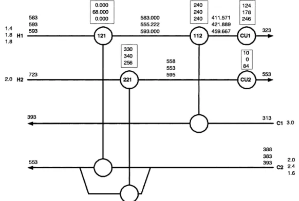
1. Iteration 1. To start, by applying the nominal
conditions to eqs 2-4, a network with a minimum TAC
of $25,958$/year is obtained, and its structure and the data on flow rate and temperature are shown in Figure 3, where the heat-exchange load for each unit is boxed. Let SN1 ) {z
112 1
, z2111 , z2211 , zcu11} denote the set of selected units of the first candidate network. The constraints in eqs 6 and 7 are then utilized to examine this network. Because there are six equations and six unknowns, no variable is left for control (i.e., nu) 0).
Solving the nonlinear programming problem, eq 11, for each active set of constraints results in the flexibility index value of F ) 0.1311 (details of the evaluation can be found in Appendix A). Such a low value of the flexibility index implies that the network structure designed for the base case will be infeasible for some possible input conditions within the disturbance range. Thus, to obtain a better network, an additional param-eter point that embraces the maximum total heat-exchange load (i.e., FH1U, FC2U, TH1U, TC2L ) and the integer cut, eq 15, with SN1and n
SN
1 ) 4 to exclude the current
network configuration are appended to the network synthesis problem.
2. Iteration 2. With the integer cut for excluding the
current network obtained from iteration 1, eqs 2-4 are solved again by also considering the conditions of period 1 as well as the nominal operating case. The resulting network, shown in Figure 4, features a TAC of $35,-219$/year, with the set of selected units SN2 ) {z
122 2 , z2112 , z2212 , zcu12}and nSN2 ) 4. Equations 6 and 7 are then employed to test the operation feasibility of this network structure under the specified operating range. Here, because the numbers of equations and unknowns are the same (six equations and six unknowns), no ad-ditional control variable is left (nu) 0). The solution of
the nonlinear programming problem, eq 11, again shows that F ) 0.1847 is still less than 1, and therefore, the network is again unqualified. Appendix A shows the detailed evaluation procedures. Once again, a new parameter point that embraces the maximum cooling load (i.e. FH1U, FC2L , TH1U , TC2U) and the integer cuts to rule out the same networks obtained from the first and the second iterations are introduced into the search space. Next comes the third iteration.
3. Iteration 3. From the same eqs 2-4 with the
application of the nominal operating conditions and
Table 2. Nominal and Multiperiod Operating Conditions for Example 1a process streams heat-capacity flow rate FCp (kW/K) input temperature Tin(K) output temperature Tout(K)
nominal conditions (base case)
hot stream 1 (H1) 1.4 583 323 hot stream 2 (H2) 2.0 723 553 cold stream 1 (C1) 3.0 313 393 cold stream 2 (C2) 2.0 388 553 hot utility (HU) - 573 573 cold utility (CU) - 303 323
period 1 (maximizing exchange area)
hot stream 1 (H1) 1.8 593 323 hot stream 2 (H2) 2.0 723 553 cold stream 1 (C1) 3.0 313 393 cold stream 2 (C2) 2.4 383 553
period 2 (including maximum cooling load) hot stream 1 (H1) 1.8 593 323 hot stream 2 (H2) 2.0 723 553 cold stream 1 (C1) 3.0 313 393 cold stream 2 (C2) 1.6 393 553
period 3 (including maximum heating load) hot stream 1 (H1) 1.0 573 323 hot stream 2 (H2) 2.0 723 553 cold stream 1 (C1) 3.0 313 393 cold stream 2 (C2) 2.4 383 553
a∆T
min) 10 K. U ) 0.08 (kW m-2K-1) for all matches.
periods 1 and 2 and the integer cuts for excluding the networks obtained from iterations 1 and 2, a new configuration is generated as shown in Figure 5. It features a TAC of $37,274$/year and the set of selected units SN3 ) {z 112 3 , z 121 3 , z 221 3 , zcu 1 3, zcu 2 3}with n SN 3 ) 5.
Note that one additional cooler is joined because of the inclusion of maximizing the cooling load. To test for the feasibility of operation of this network, we found that there are seven equations and eight unknowns in constraint eqs 6 and 7; accordingly, one variable, say, qcu2, is selected as the control variable. A flexibility
index value of F ) 0.6358 is found by solving the nonlinear programming problem, eq 11, for each pos-sible active set of constraints. Seeing that the network configuration is still less than feasible, in preparation for the next iteration, a new parameter point with the
maximum heating load (i.e., FH1L , FC2U, TH1L , TC2L ) is added, and the integer cuts are implemented to exclude networks 1-3 from consideration. The fourth iteration is then performed.
4. Iteration 4. Taking the nominal operating
condi-tions and periods 1-3 into consideration simultaneously and including the three integer cuts for excluding networks 1-3 in solving eqs 2-4 leads to the network shown in Figure 6. The TAC is $41,876$/year, and SN4
) {z1124 , z1214 , z2214 , zcu14, zcu24, zhu14} with nSN4 ) 6. Notably, one heater is added because of the additional consideration of maximizing the heating load. This time, there are eight equations and 10 unknowns in eqs 6 and 7 for flexibility test; thus, two control variables are selected, say, qcu1and qcu2. Then, solving the nonlinear
Figure 4. HEN structures for example 1 when considering the nominal conditions and period 1 for synthesis.
programming problem, eq 11, for each active set of constraints results in F ) 1.7134. This value indicates that the network structure derived from the fourth synthesis step is not only economical, but also feasible for the overall operating space, which terminates the whole search process. The annual capital cost, the operating cost, the total annual cost, and the flexibility of resulting networks for example 1 are reported in Table 3 for comparison.
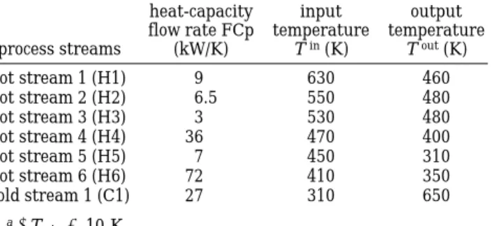
Example 2. A Six-Hot/One-Cold Streams Prob-lem. This problem consists of six hot streams and one
cold stream (NH) 6, NC) 1), along with fuel and cooling
water as utilities. The problem data are listed in Tables 4 and 5. Overall heat-transfer coefficients for process matches, Uij[kW/(m2K)], are U11) 0.6, U21) 0.4, U31
) 0.3, U41) 0.4, and U61) 0.3, and those for cold utility
matches, Ucui, are Ucu1) 0.1, Ucu5) 0.3, and Ucu6)
0.4. The minimum number of superstructure stages is NT) 6, as suggested.3The desired range for uncertain
disturbances are assigned to be FCp ) FCp(0) ( 10%
and Tin) Tin(0)( 10 K for all hot/cold streams. Solving
eqs 2-4 for the base case gives a network with a TAC of $863,071$/year and selected units of SN1 ) {z
111 1 , z2111 , z3121 , z4131 , z6141 , zcu11, zcu51, zcu61, zhu11}, as shown in Figure 7. Constraint eqs 6 and 7 are then used to scrutinize the flexibility of this network. Given that there are 13 equations and 15 unknowns, two control variables (nu) 2) can be selected, say, qcu1and qcu6. A
satisfactory value of F ) 1.2014 is obtained from solving the nonlinear programming problem, eq 11, for each active set of constraints, so this network structure derived from the synthesis step is both economical and feasible for the full disturbance range. The costs and the flexibility of the network obtained via simultaneous design are reported in Table 6 for comparison with the result of sequential design.11
Figure 6. HEN structures for example 1 when considering the nominal conditions and periods 1-3 for synthesis. Table 3. Comparison of the Annual Capital Costs,
Operating Costs, Total Annual Costs, and Flexibilities of the Resulting Networks for Example 1
annual capital
cost operatingcost total annual
cost flexibility
nominal 19,019 6,981 26,000 0.1311
nominal + period 1 27,092 8,127 35,219 0.1847 nominal + periods 1 and 2 26,125 11,149 37,274 0.6358 nominal + periods 1-3 30,104 11,772 41,876 1.7134 sequential 39,380 10,499 49,879 1.0 Table 4. Cost Data for Example 2
cost parameter value
fuel cost 204.732× 10⁻⁴$/kWh
cooling water cost 60.576× 10⁻⁴$/kWh operating time 8,600 h/year exchanger capital costa 4,333A0.6
furnace cost 191.94(qhu)0.7
capital annual factor 0.2
aA ) exchanger area (m2).
Table 5. Nominal Conditions for Example 2a
process streams heat-capacity flow rate FCp (kW/K) input temperature Tin(K) output temperature Tout(K) hot stream 1 (H1) 9 630 460 hot stream 2 (H2) 6.5 550 480 hot stream 3 (H3) 3 530 480 hot stream 4 (H4) 36 470 400 hot stream 5 (H5) 7 450 310 hot stream 6 (H6) 72 410 350 cold stream 1 (C1) 27 310 650 a∆T min) 10 K.
Table 6. Comparison of the Capital Costs, Operating Costs, Total Annual Costs, and the Flexibilities of the Resulting Networks for Example 2
annual capital cost operating cost total annual cost flexibility simultaneous 107,991 755,080 863,071 1.2014 sequential 126,566 744,244 870,810 1.0
7. Conclusion
In this paper, a new strategy has been proposed to synthesize flexible heat-exchange networks that in-volves uncertain source-stream temperatures and flow rates. The design problem is decomposed into iterative steps: First, the MINLP formulation is applied for the synthesis of a network configuration that bears the minimum total annual cost, with consideration of a finite number of extreme operating points that tend to maximize the need for heat exchangers, coolers, and heaters. Second, the active set strategy is employed for the flexibility analysis to test the operational feasibility of the resulting network over the full range of expected variations of the source-stream temperatures and flow rates. If the network structure does not meet the assigned flexibility target, then the current network is excluded by appending some integer cuts to the feasible network search space, and then the search process reverts to the synthesis step to find a new candidate network. Sometimes, several iterations are required to determine the final qualified network. By means of the two aforementioned numerical examples, we demon-strate that the proposed new demon-strategy can generate a feasible network for uncertain supply temperatures and flow rates in a relatively more efficient way.
Acknowledgment
This work is supported by the National Science Council (ROC) under Contract NSC91-ET-7-002-004-ET. Partial financial support of the Ministry of Eco-nomic Affairs under Grant 92-EC-17-A-09-S1-019 is also acknowledged.
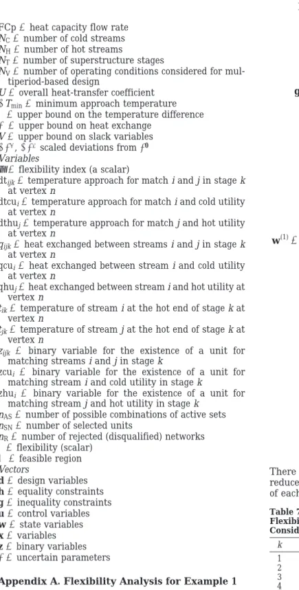
Nomenclature Indices
i ) hot process stream j ) cold process stream k ) superstructure stage
n ) multiperiod limiting operating conditions Sets
AS(k) ) kth index set of active constraints CI ) index set of condensed inequalities CP ) set of cold process stream
HP ) set of hot process streams
NAS) set of all possible combinations of active constraints SN ) set of selected units
ST ) set of superstructure stages
VT ) set of multiperiod operating conditions (base case included)
Parameters
Tin) inlet temperature of stream
Tout) outlet temperature of stream
FCp ) heat capacity flow rate NC) number of cold streams
NH) number of hot streams
NT) number of superstructure stages
NV) number of operating conditions considered for mul-tiperiod-based design
U ) overall heat-transfer coefficient ∆Tmin) minimum approach temperature Γ ) upper bound on the temperature difference Λ ) upper bound on heat exchange
V ) upper bound on slack variables ∆θ-, ∆θ+scaled deviations from θ0
Variables
F ) flexibility index (a scalar)
dtijk) temperature approach for match i and j in stage k
at vertex n
dtcui) temperature approach for match i and cold utility
at vertex n
dthuj) temperature approach for match j and hot utility
at vertex n
qijk) heat exchanged between streams i and j in stage k
at vertex n
qcui) heat exchanged between stream i and cold utility
at vertex n
qhuj) heat exchanged between stream i and hot utility at
vertex n
tik) temperature of stream i at the hot end of stage k at
vertex n
tjk) temperature of stream j at the hot end of stage k at
vertex n
zijk ) binary variable for the existence of a unit for
matching streams i and j in stage k
zcui ) binary variable for the existence of a unit for
matching stream i and cold utility in stage k
zhui ) binary variable for the existence of a unit for
matching stream j and hot utility in stage k nAS) number of possible combinations of active sets
nSN) number of selected units
nR) number of rejected (disqualified) networks
δ ) flexibility (scalar) Ω ) feasible region Vectors d ) design variables h ) equality constraints g ) inequality constraints u ) control variables w ) state variables x ) variables z ) binary variables θ ) uncertain parameters
Appendix A. Flexibility Analysis for Example 1 1. Iteration 1. The equalities/inequalities, state
variables, and reduced inequalities for the network of example 1 when considering the nominal conditions for synthesis are as follows
There are 10 possible active sets in this case. The reduced inequalities and the associated flexibility index of each active set are listed in Table 7.
2. Iteration 2. The equalities/inequalities, state
variables, and reduced inequalities for the network of example 1 when considering the nominal conditions and period 1 for synthesis are as follows
h(1)(d,u,w,θ) )
{
q112- (TH1 in - t H1,3)FCpH1 q112- (tC1,2- 313) × 3 q211- (393 - tC1,2)× 3 q221- (553 - TC2 in )FCpC2 q211+ q221- (723 - 553) × 2 qcu1- (tH1,3- 323)FCpH1}
) 0 (16) g(1)(d,u,w,θ) ){
tH1,3- TH1 in 323 - tH1,3 tC1,2- 393 313 - tC1,2 TC2in - 553 ∆Tmin+ tC1,2- TH1 in ∆Tmin+ 313 - tH1,3 ∆Tmin+ 323 - tH1,3 ∆Tmin+ tC1,2- 723 ∆Tmin+ TC2 in - 553}
e 0 (17) w(1)){
w1 w2 w3 w4 w5 w6}
){
q221 q211 tC1,3 q112 tH1,3 qcu1}
){
(553 - TC2in)FCpC2 (723 - 553)× 2 - w1 393 -w2 3 (w3- 313) × 3 TH1in - w4 FCpH1 (w5- 323)FCpH1}
(18) f(1)(d,u,θ) ){
w5- TH1in 323 - w5 w3- 393 313 - w3 TC2 in - 553 ∆Tmin+ w3- TH1 in ∆Tmin+ 313 - w5 ∆Tmin+ 323 - w5 ∆Tmin+ w3- 723 ∆Tmin+ TC2 in - 553}
e 0 (19)Table 7. Reduced Inequalities and the Associated Flexibility Index of Each Active Set for Example 1 When Considering the Nominal Data in Network Synthesis
k AS(k) δk k AS(k) δk 1 f1 3.3156 6 f6 4.7610 2 f2 0.6957 7 f7 0.6957 3 f3 0.1311 8 f8 0.6358 4 f4 3.3156 9 f9 5.3105 5 f5 33.000 10 f10 33.000 h(2)(d,u,w,θ) )
{
q122- (TH1in - tH1,3)FCpH1 q122- (tC2,2- TC2in)FCpC2 q211+ q221- (723 - 553) × 2 q211- (393 - 313) × 3 q221- (553 - tC2,2)FCpC2 qcu1- (tH1,3- 323)FCpH1}
) 0 (20)The reduced inequalities and the associated flexibility index of each active set are reported in Table 8.
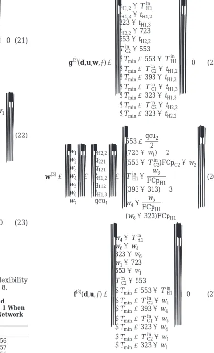
3. Iteration 3. The equalities/inequalities, state
variables, and reduced inequalities for the network of example 1 when considering the nominal conditions and periods 1 and 2 for synthesis are as follows
The signs of the sensitivities for these reduced inequali-ties to the control variable, the inequaliinequali-ties, and the associated flexibility index of each active set are re-ported in Tables 9 and 10.
4. Iteration 4. The equalities/inequalities, state
variables, and reduced inequalities for the network of example 1 when considering the nominal conditions and
g(3)(d,u,w,θ) )
{
tH1,2- TH1 in tH1,3- tH1,2 323 - tH1,3 tH2,2- 723 553 - tH2,2 TC2in - 553 ∆Tmin+ 553 - TH1in ∆Tmin+ TC2in - tH1,2 ∆Tmin+ 393 - tH1,2 ∆Tmin+ TC1in - tH1,3 ∆Tmin+ 323 - tH1,3 ∆Tmin+ TC2in - tH2,2 ∆Tmin+ 323 - tH2,2}
e 0 (25) w(3)){
w1 w2 w3 w4 w5 w6 w7}
){
tH2,2 q221 q121 tH1,2 q112 tH1,3 qcu1}
){
553 +qcu2 2 (723 - w1)× 2 (553 - TC2in)FCpC2- w2 TH1in - w3 FCpH1 (393 - 313)× 3 w4- w5 FCpH1 (w6- 323)FCpH1}
(26) f(3)(d,u,θ) ){
w4- TH1in w6- w4 323 - w6 w1- 723 553 - w1 TC2 in - 553 ∆Tmin+ 553 - TH1in ∆Tmin+ TC2in - w4 ∆Tmin+ 393 - w4 ∆Tmin+ TC1in - w6 ∆Tmin+ 323 - w4 ∆Tmin+ TC2in - w1 ∆Tmin+ 323 - w1}
e 0 (27)Table 9. Signs of Dfm/Dqcu2for Example 1 When
Considering the Nominal Data and Periods 1 and 2 in Network Synthesis ∂fm/∂qcu2 >0 <0 )0 f3 f1 f2 f4 f5 f6 f8 f12 f7 f9 f13 f10 f11 g(2)(d,u,w,θ) )
{
tH1,3- TH1 in 323 - tH1,3 TC2in - tC2,2 tC2,2- 553 ∆Tmin+ tC2,2- TH1 in ∆Tmin+ TC2 in - t H1,3 ∆Tmin+ 323 - tH1,3 ∆Tmin+ tC2,2- 553}
e 0 (21) w(2)){
w1 w2 w3 w4 w5 w6}
){
q211 q221 tC2,2 q122 tH1,3 qcu1}
){
(393 - 313)× 3 (723 - 553)× 2 - w1 553 - w2 FCpC2 (w3- TC2in)FCpC2 TH1in - w4 FCpH1 (w5- 323)FCpH1}
(22) f(2)(d,u,θ) ){
w5- TH1 in 323 - w5 TC2in - w3 w3- 553 ∆Tmin+ w3- TH1 in ∆Tmin+ TC2 in - w 5 ∆Tmin+ 323 - w5 ∆Tmin+ w3- 553}
e 0 (23)Table 8. Reduced Inequalities and the Associated Flexibility Index of Each Active Set for Example 1 When Considering the Nominal Data and Period 1 in Network Synthesis k AS(k) δk 1 f1 3.3156 2 f2 0.6957 3 f3 3.3156 4 f4 -5 f5 4.6033 6 f6 0.1847 7 f7 0.6358 8 f8 20.000 h(3)(d,u,w,θ) )
{
q121- (TH1in - tH1,2)FCpH1 q112- (tH1,2- tH1,3)FCpH1 q112- (393 - 313)FCpC1 q221- (723 - tH2,2)× 2 q121+ q221- (553 - TC2 in )FCpC2 qcu1- (tH1,3- 323)FCpH1 qcu2- (tH2,2- 553)FCpH2}
) 0 (24)periods 1-3 for synthesis are as follows The signs of the sensitivity function for these inequali-ties to the control variable are reported in Tables 9-12. With two control variables, there are more than 100 possible combinations of active sets. The inequalities and the associated flexibility indices of the active sets are listed in Table 12.
Literature Cited
(1) Linnhoff, B.; Hindmarsh, E. The pinch design method for heat exchanger networks. Chem. Eng. Sci. 1983, 38, 745.
(2) Floudas, C. A.; Ciric, A. R.; Grossmann, I. E. Automatic Synthesis of Optimum Heat Exchanger Network Configurations.
AIChE J. 1986, 32, 276.
(3) Yee, T. F.; Grossmann, I. E.; Kravanja, Z. Simultaneous optimization models for heat integration-I. Area and energy targeting and modeling of multi-stream exchangers. Comput.
Chem. Eng. 1990, 14, 1151.
(4) Yee, T. F.; Grossmann, I. E. Simultaneous optimization models for heat integration-II. Heat exchanger network synthesis.
Comput. Chem. Eng. 1990, 14, 1165.
(5) Grossmann, I. E.; Caballero, J. A.; Yeomans, H. Mathemati-cal programming approaches to the synthesis of chemiMathemati-cal process systems. Korean J. Chem. Eng. 1999, 16 (4), 407.
(6) Furman, K. C.; Sahinidis, N. V. A critical review and annotated bibliography for heat exchanger network synthesis in the 20th century. Ind. Eng. Chem. Res. 2002, 41, 2335.
g(4)(d,u,w,θ) )
{
tH1,2- TH1 in tH1,3- tH1,2 323 - tH1,3 tH2,2- 723 553 - tH2,2 313 - tC1,2 tC1,2- 393 ∆Tmin+ 553 - TH1in ∆Tmin+ TC2in - tH1,2 ∆Tmin+ tC1,2- tH1,2 ∆Tmin+ 313 - tH1,3 ∆Tmin+ 323 - tH1,3 ∆Tmin+ TC2in - tH2,2 ∆Tmin+ 323 - tH2,2 ∆Tmin+ tC1,2- 573}
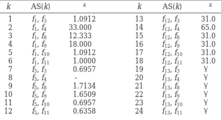
e 0 (29)Table 10. Reduced Inequalities and Associated Flexibility Indexes of Each Active Set for Example 1 When Considering the Nominal Data and Periods 1 and 2 in Network Synthesis k AS(k) δk k AS(k) δk 1 f1, f3 1.0912 13 f12, f3 31.0 2 f1, f4 33.000 14 f12, f4 65.0 3 f1, f8 12.333 15 f12, f8 31.0 4 f1, f9 18.000 16 f12, f9 31.0 5 f1, f10 1.0912 17 f12, f10 31.0 6 f1, f11 1.0000 18 f12, f11 31.0 7 f5, f3 0.6957 19 f13, f3 -8 f5, f4 - 20 f13, f4 -9 f5, f8 1.7134 21 f13, f8 -10 f5, f9 1.6509 22 f13, f9 -11 f5, f10 0.6957 23 f13, f10 -12 f5, f11 0.6358 24 f13, f11 -h(4)(d,u,w,θ) )
{
q121- (TH1 in - t H1,2)FCpH1 q221- (723 - tH2,2)× 2 q121+ q221- (553 - TC2in)FCpC2 q112- (tH1,2- tH1,3)FCpH1 q112- (tC1,2- 313)FCpC1 qcu1- (tH1,3- 323)FCpH1 qcu2- (tH2,2- 553)FCpH2 qhu1- (393 - tC1,2)FCpC1}
) 0 (28) w(4)){
w1 w2 w3 w4 w5 w6 w7 w8}
){
tH1,3 tH2,2 q221 q121 tH1,2 q112 tC1,2 qhu1}
){
323 + qcu1 FCpH1 553 +qcu2 2 (723 - w2)× 2 (553 - TC2in)FCpC2- w3 TH1in -w4 FCpH1 (w5- w1)FCpH1 313 +w6 3 (393 - w7)× 3}
(30) f(4)(d,u,θ) ){
w5- TH1 in w1- w5 323 - w1 w2- 723 553 - w2 313 - w7 w7- 393 ∆Tmin+ 553 - TH1in ∆Tmin+ TC2in - w5 ∆Tmin+ tC1,2- w5 ∆Tmin+ 313 - w1 ∆Tmin+ 323 - w1 ∆Tmin+ TC2in - w2 ∆Tmin+ 323 - w2 ∆Tmin+ w7- 573}
e 0 (31)Table 11. Signs of Dfm/Dqcu1and Dfm/Dqcu2for Example 1
When Considering the Nominal Data and Periods 1-3 in Network Synthesis ∂fm/∂qcu1 ∂fm/∂qcu2 >0 <0 )0 >0 <0 )0 f2 f3 f1 f2 f1 f3 f6 f7 f4 f4 f5 f8 f10 f5 f6 f7 f11 f11 f8 f9 f13 f12 f12 f9 f10 f14 f15 f13 f15 f14
Table 12. Reduced Inequalities and Associated Flexibility Indexes for Some Active Sets for Example 1 When Considering the Nominal Data and Periods 1-3 in Network Synthesis k AS(k) δk 1 f1, f5, f9 -2 f2, f5, f9 1.7134 3 f3, f5, f9 1.7134 4 f4, f5, f9 -5 f5, f6, f9 1.7134 6 f5, f7, f9 5.5310 7 f5, f9, f10 5.5354 8 f5, f9, f11 1.7134 9 f5, f9, f13
(7) Marselle, D. F.; Morari, M.; Rudd, D. F. Design of resilient processing plants-II: Design and control of energy management systems. Chem. Eng. Sci. 1982, 37, 259.
(8) Grossmann, I. E.; Halemane, K. P.; Swaney, R. E., Optimi-zation strategies for flexible chemical process. Comput. Chem. Eng.
1983, 439.
(9) Swaney, R. E.; Grossmann, I. E. An index for operational flexibility in chemical process design. Part I. Formulation and theory. AIChE J. 1985, 31, 621.
(10) Grossmann, I. E.; Floudas, C. A. Active constraint strategy for flexibility analysis in chemical processes. Comput. Chem. Eng.
1987, 11, 675.
(11) Floudas, C. A.; Grossmann, I. E. Synthesis of flexible heat exchanger networks with uncertain flowrates and temperatures.
Comput. Chem. Eng. 1987, 11, 319.
(12) Aaltola, J. Simultaneous synthesis of flexible heat ex-changer network. Appl. Therm. Eng. 2002, 22, 907.
(13) Halemane, K. P.; Grossmann, I. E. Optimal process design under uncertainty. AIChE J. 1983, 29, 425.
(14) Floudas, C. A. Nonlinear and Mixed-Integer
Optimiza-tion: Fundamentals and Applications; Oxford University Press:
New York, 1995.
(15) Biegler, L. T.; Grossmann, I. E.; Westerberg, A. W.
Systematic Methods of Chemical Process Design; Prentice Hall:
Upper Saddle River, NJ, 1997.
(16) Chen, J. J. J. Letter to the editor: Comments on improve-ment on a replaceimprove-ment for the logarithmic mean. Chem. Eng. Sci.
1987, 2488.
(17) Konukman, A. E. S.; Camurdan, M. C.; Akman, U. Simultaneous flexibility targeting and synthesis of minimum-utility heat-exchanger networks with superstructure-based MILP formulation. Chem. Eng. Process. 2002, 41, 501.
(18) Brooke, A.; Kendrick. D.; Meeraus, A.; Raman, R.; Rosenthal, R. E. GAMS: A User’s Guide; Scientific Press: Redwood City, CA, 1998.
Received for review September 2, 2003 Revised manuscript received May 28, 2004 Accepted June 9, 2004