High-order MS_CMAC neural network

High-Order MS_CMAC Neural Network

J. C. Jan and Shih-Lin Hung

Abstract—A macro structure cerebellar model articulation controller (CMAC) or MS_CMAC was developed by connecting several one-dimensional (1-D) CMACs as a tree structure, which decomposes a multidimensional problem into a set of 1-D subprob-lems, to reduce the computational complexity in multidimensional CMAC. Additionally, a trapezium scheme is proposed to assist MS_CMAC to model nonlinear systems. However, this trapezium scheme cannot perform a real smooth interpolation, and its working parameters are obtained through cross-validation. A quadratic splines scheme is developed herein to replace the trapezium scheme in MS_CMAC, named high-order MS_CMAC (HMS_CMAC). The quadratic splines scheme systematically transforms the stepwise weight contents of CMACs in MS_CMAC into smooth weight contents to perform the smooth outputs. Test results affirm that the HMS_CMAC has acceptable generalization in continuous function-mapping problems for nonoverlapping association in training instances. Nonoverlapping association in training instances not only significantly reduces the number of training instances needed, but also requires only one learning cycle in the learning stage.

Index Terms—Cerebellar model articulation controller (CMAC), high-order MS_CMAC, macro structure cerebellar model articulation controller (MS_CMAC), quadratic splines.

I. INTRODUCTION

T

(CMAC), a supervised neural-network learning model developed by Albus [1], [2], is employed mainly in the control domain [3]–[5]. The original Albus CMAC (or the simple CMAC as it will be subsequently termed) produces a linear interpolation by using the binary basis function as a generalization scheme. Consequently, the output is constant within each quantized state and the derivative information is not preserved. For precisely modeling continuous functions, Moody [6] proposed using the graded neighborhood response functions (linear basis functions) in CMAC to perform con-tinuous interpolation. Meanwhile, Lane et al. [7] developed a higher order CMAC neural network which uses the B-spline functions to replace the binary basis functions. In employing these functions, the method of updating weights distributes errors among the assigned weights according to the intensity of the B-spline functions. Additionally, Chiang and Lin [8] employed Gaussian basis functions as a generalization scheme. The Gaussuan basis function CMAC has been affirmed to be capable of learning both functions and function derivatives.

Generally, the CMAC requires extensive memory for map-ping multidimensional functions. Lin and Li [9] proposed a CMAC structure comprising numerous small CMACs to learn a

Manuscript received September 3, 1999; revised May 25, 2000 and December 18, 2000.

The authors are with the Department of Civil Engineering, National Chiao Tung University, Hsinchu, Taiwan 300, R.O.C.

Publisher Item Identifier S 1045-9227(01)03715-8.

multi-dimensional function-mapping problem. In doing so, they intended to solve the fast size-growing problem and the learning difficulty in currently available types of neural networks. In their work, the network structure is always a three-layer tree structure. The root is the sum of the outputs of the nodes in the second level, called the submodules. Submodules are the multiplication of the outputs from the third level, which is a set of combinative small CMACs. Recently, Hung and Jan [10] developed a macro structure CMAC (MS_CMAC) neural network in structural engineering. The MS_CMAC represents a tree-based aggregate of one-dimensional (1-D) simple CMACs, where the ensemble is trained with a simplified time inversion technique borrowed from Albus’ work [2]. The topology of the tree structure depends on a set of combinative training instances. Rather than employing a high-order basis function to enhance the prediction accuracy of MS_CMAC in nonlinear systems, a trapezium scheme is proposed in MS_CMAC. The trapezium scheme modifies the stepwise weight contents of CMACs in MS_CMAC into the trapezium-wise weight contents once each CMACs linear optimization process is complete. The trapezium scheme has been demonstrated to be able to provide pseudosmooth outputs in mapping continuous functions [10]. However, their scheme is limited to a cross-val-idation working parameter.

This work presents a quadratic splines scheme to upgrade the MS_CMAC, and called the high-order MS_CMAC (HMS_CMAC) neural-network model. The proposed scheme systematically alters the stepwise weight contents of CMACs in MS_CMAC into the smooth weight contents. The aim is not only to obtain smooth outputs but also to use a few training instances to achieve acceptable training. An illus-trative example, three-variable functional mapping problem, demonstrates the effectiveness of the learning performance of the HMS_CMAC models. The HMS_CMAC model is implemented with MATLAB [11] on a personal computer.

II. SIMPLECMACANDTIMEINVERSIONCMAC

A. Simple CMAC

The simple CMAC learning algorithm is implemented mainly via three sequential mappings in four multidimensional spaces: input state space , association memory space , phys-ical memory space , and output space . The learning stage in a simple CMAC progresses via three sequential mappings as follows. The first mapping is between input space and association memory space . In this step, the vector in space is mapped to an association vector in space . The vector contains elements, where is termed generalization size. The next mapping is between association memory space and physical memory space . Any vector in is mapped to an active physical memory . The third mapping is between

physical memory space and output space . In a simple CMAC neural network, a function of linear combinations of the physically addressed memory in is used in this mapping. Therefore, the output is calculated by summing the physically addressed memory in as follows:

(1)

where denotes the th vector of . Similar to other su-pervised neural network learning models, the computed output is compared to the desired output . If the difference be-tween the computed and desired outputs exceeds a predefined threshold, the in (1) is updated [1]. The learning phase is terminated when the predefined stopping criterion is satisfied. After the learning stage is completed, the output of any given instance is directly computed via (1).

The simple CMAC produces a nonsmooth response owing to its binary basis function. High-order basis functions, such as the B-spline function [7], have been used in generalization schemes to obtain smoother weight contents. This approach attempts to find a smooth weight content in physical memory which pro-vides a superior generalization in continuous functional map-ping problems.

B. Time Inversion CMAC

Albus [2] proposed a time inversion technique to optimize the simple CMAC in multidimensional problems. Herein, the time inversion CMAC is developed using a simplified time inversion technique borrowed from Albus’ work [2]. For example, given a set of instances with the six input variables and corresponding output , plus an unsolved instance (verification instance) with the input , then the time inversion CMAC, combined by sequentially connecting two simple CMACs, can be briefly

described as follows. 1) and are

used to train the first simple CMAC of the time inversion CMAC according to the aforementioned three sequential mappings. The weight of the first simple CMAC is then obtained after the CMAC is successfully trained. 2) Compute the outputs corresponding to some specific instances of

input through the first CMAC with

weight . Herein, the instances

are termed transition instances. 3) These transition instances, , are then used for training the second simple CMAC in the time inversion CMAC. Consequently, the weight of the second simple CMAC is obtained. Finally,

the output corresponding to can be

computed through the second CMAC with weight . III. HMS_CMAC

A. MS_CMAC

The underlying notion of MS_CMAC is to decompose a multidimensional problem into a set of 1-D subproblems [10]. The MS_CMAC learning algorithm is briefly reviewed below. Assume a set of combinative training instances is

given. denotes the input, and the

corresponding output comprises -data. Each input element where

and the subscript represents the number of elements in the combination of . According to these training instances, the topology of the MS_CMAC neural network, an -level tree structure, is then determined [10]. To further depict the tree structure, a three-input combinative example is utilized to illustrate how to construct the MS_CMAC tree structure. In this example, represents a training instance. The following combinations of three elements for , , and , respectively, are considered as training instances:

where and where and where and

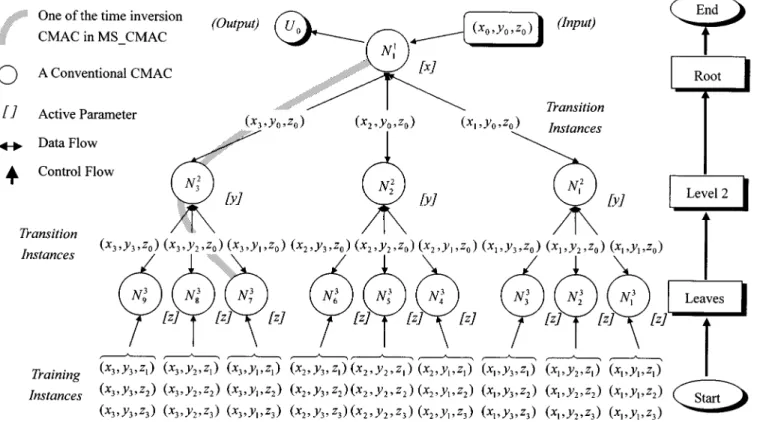
Now, an MS_CMAC with a three-level tree structure is em-ployed for the case, and is illustrated in Fig. 1. Thee nodes ( , and ) exist in the second level and nine nodes ( ) in the third level. Once the tree structure is set, the corresponding output of any new instance can be solved via the MS_CMAC neural network through the following steps:

Step 1) Instance is used as a verification instance in the node (root). The training instances are divided into groups and fed to nodes (leaves).

Herein, denotes the

th training instance chosen from the training in-stance base for node . The input element for is defined as:

for to for to

The subscript is determined as follows:

for downto if then else if else (2) In Fig. 1, the three training instances ,

and are assigned to

, the three training instances ,

and are assigned to

, and so on. Notably, the and elements are identical in leaves. Consequently, the leaves are practically to solve a one-dimensional problem ( -element). Herein, the -element is defined as the

active parameter in the third level.

Step 2) Generate transition instances for the nodes from levels to 2. Each node in the tree has a transition instance, except for the root. The transition instance

Fig. 1. The topology of a three-level MS_CMAC neural-network model.

is used to verify and train the node and the node’s parent, respectively. The transition instance of (for to 2) is defined as follows:

(3)

where

identity matrix;

input of any training instance of node ; input of the verification instance of the root; input of the transition instance of node .

The and variables of the transition instance corre-sponding to are the same as those of the training instances in , and the variables of the tran-sition and verification instances are also the same. Similarly, the variables of the transition instance and the training instances corresponding to are identical, and the and variables of the transition instance are the same as those of the verification in-stance. Consequently, the active parameters for the first and second levels are the -element and -ele-ment, respectively.

Step 3) Perform the learning and verification stages for all CMACs (nodes) from leaves to root, sequentially.

B. Quadratic Splines Scheme for Smoothing Weight Contents

Our previous work [10] adopted a trapezium scheme to assist MS_CMAC to model nonlinear systems instead of using high-order basis functions. The trapezium scheme attempts to modify stepwise weight content of CMACs in MS_CMAC after

the linear optimization processes of CMACs are completed. The trapezium scheme has been confirmed to be effective in enhancing the prediction accuracy of MS_CMAC in nonlinear function-mapping problems [10]. However, obtaining proper working parameters for all 1-D CMACs in MS_CMAC is very difficult. Additionally, the trapezium scheme is only an approx-imate method and does not produce truly smooth outputs.

Accordingly, a quadratic splines scheme is developed to re-place the trapezium scheme. Assume that the value of modi-fied physical memory is defined as a quadratic spline

in the interval and . The constants , , and in any quadratic spline could be determined via the following conditions.

For to , the boundary conditions for each quadratic spline are as follows:

1) The areas between the interval of and must be equal for both the quadratic spline and the step function:

.

2) The function must be continuous across each spline boundary; that is, the function values at (for to

) must be equal: .

3) The function must be smooth at the boundary of two con-junct splines; that is, the first derivatives at (for

to ) must be equal: .

Hence, boundary conditions are derived. The linear system has unknowns, but only independent equa-tions are available. Two more boundary condiequa-tions are required to solve the linear system of equations. Herein, and are assumed to be equal to zero. Consequently, the physical memory is now modified as a set of quadratic spline functions.

(a) (b)

(c) (d)

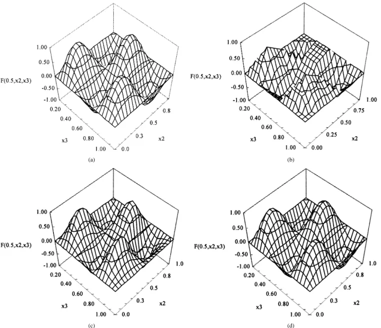
Fig. 2. (a) The plots ofF (0:5; x ; x ). (b) The computed output of F (0:5; x ; x ) in MS_CMAC ( = 0). (c) The computed output of F (0:5; x ; x ) in MS_CMAC ( = 0:8). (d) The computed output of F (0:5; x ; x ) in HMS_CMAC.

Since the weight content is transformed from a discrete-type into a continuous type, the output is computed via the following equation:

(4)

C. Flow of HMS_CMAC

Herein, the HMS_CMAC is constructed via a tree-based structure CMAC with a quadratic splines scheme. Assume that one input set of combinative training data is given and defined

as , then the set is transformed

into the integer space as . Where

term is the generalization size. Notably, the value of can be arbitrarily defined ( ) in an HMS_CMAC. Moreover, nonoverlapping association memory exists between training instances.

The computation in HMS_CMAC progresses from leaves to root and includes two stages in each node, the learning stage and the operation stage (1-D simple CMAC). The learning stage involves two steps. First, perform linear optimization. Second, after the linear optimization process is complete, smooth step-wise weight content via the quadratic splines scheme. Mean-while, the operation stage involves calculating outputs using (4). The flow of HMS_CMAC for mapping an -variable function is listed as follows.

1) Construct an -level tree-based structure CMAC ac-cording to a set of combinative training instances. 2) Divide training instances into several groups for the

leaves using (2).

3) Generate transition instances via (3). 4) Perform learning stages in leaves off-line. 5) Execute the operation stage in leaves on-line.

6) Perform learning and operation stages from level to root on-line.

TABLE I

COMPARISON OFCMAC MODELS

IV. ILLUSTRATIVEEXAMPLE

An illustrative example, mapping a three-variable nonlinear function, is employed to demonstrate the effectiveness of the learning performance of the HMS_CMAC model. The three-variable function is defined as follows:

for

Assume that the values of the three elements , , and are in the interval 0 to 1, respectively, and are linearly transformed into the inputs , , and in the integer interval 0 to 100. Consequently, a total of 1 030 301 ( ) distinct data exist in the learning domain. To train the neural network, the following combinations of three inputs are selected as training instances:

The 216 ( ) training instances are used to train the

HMS_CMAC for mapping the function .

Additionally, a set of 200 instances is randomly selected for verification. According to the combinative training instances, the topology of the HMS_CMAC neural network is a three-level tree structure including one node in level 1 (root), six nodes in level 2, and 36 nodes in level 3. The active parameters for levels 1 to 3 are set as , , and , respectively.

For comparison, two MS_CMAC with trapezium scheme ( and ) are also used to map the function. Herein, the learning performance of HMS_CMAC is measured using the root mean square (rms) error and the ratio of computation time. The ratio of time for two CMAC models is defined as the ratio of computing time required by simple CMAC or MS_CMAC with trapezium scheme to that required by HMS_CMAC. Fig. 2(a) presents the plots of the function with . Fig. 2(b)–(d) show the plots corresponding to the computed output for the MS_CMAC (with

), MS_CMAC (with ), and HMS_CMAC,

respec-tively. The HMS_CMAC clearly achieves the best prediction in this example. The output of HMS_CMAC is completely smooth. In addition, Table I compares the computational time of the various models. The HMS_CMAC requires much more computational time than a simple CMAC in multidimensional function-mappings given an identical number of training instances and generalization size. The ratio of computational

time is around 0.35. However, the prediction accuracy of HMS_CMAC is significantly exceeds that of other models. To improve the prediction accuracy, an additional set of 200 training instances are randomly selected to train the simple CMAC. Thus, the number of training instances is increased to 416. Consequently, the learning time is exponentially increased, but the prediction accuracy remains poorer than that of the HMS_CMAC.

V. CONCLUSION

The work presents a novel CMAC model, named the HMS_CMAC, by utilizing a quadratic spline scheme to en-hance the prediction accuracy after the weights are updated. The quadratic splines scheme systematically alters the stepwise weight contents of CMACs in MS_CMAC into smooth weight contents to perform smooth outputs. Based on the testing results in this study, we conclude the following:

1) The quadratic splines scheme provides a novel approach to obtain the smooth weight content in a one-dimensional CMAC. The quadratic splines scheme is directly used to modify stepwise weight content, which is yielded after the simple CMAC is successfully trained, into a set of splines. 2) The linear optimization process can be completed in just one-iteration in each node of an HMS_CMAC, due to the situation of no association overlap in the learning stage. Testing results indicate that the HMS_CMAC is confirmed to have a good capacity for generalization in continuous function-mapping problems when the situation of no association memory overlap is set in the learning stage.

3) The proposed scheme reduces the number of instances re-quired for training an HMS_CMAC. Consequently, the total computational time can be significantly reduced, al-though the tree structure CMAC and splines quadratic scheme may increase computational time.

REFERENCES

[1] J. S. Albus, “A new approach to manipulator control: The cerebellar model articulation controller (CMAC),” J. Dyn. Syst., Measurement,

Contr., vol. 97, no. 3, pp. 220–227, 1975.

[2] , “Data storage in the cerebellar model articulation controller,” J.

Dyn. Syst., Measurement, Contr., vol. 97, no. 3, pp. 228–233, 1975.

[3] C. S. Lin and K. Hyongsuk, “CMAC-based adaptive critic self-organized control,” IEEE Trans. Neural Networks, vol. 2, pp. 530–533, May 1991. [4] T. W. Miller, R. P. Hewes, F. J. Glanz, and L. G. Kraft, “Real-time dy-namic control of an industrial manipulator using a neural-network-based learning controller,” IEEE Trans. Robot. Automat., vol. 6, pp. 1–9, 1990.

[5] P. C. Parks and J. Militzer, “A comparison of five algorithm for the training of CMAC memories for learning control systems,” Automat.

Remote Contr., vol. 50, pp. 254–286, 1989.

[6] J. Moody, “Fast learning in multiresolution hierarchies,” Advances

Neural Inform. Processing Syst. I, pp. 29–39, 1989.

[7] S. H. Lane, D. A. Handelman, and J. J. Gelfand, “Theory and develop-ment of higher-order CMAC neural networks,” IEEE Contr. Syst. Mag., vol. 12, no. 2, pp. 23–30, 1992.

[8] C. T. Chiang and C. S. Lin, “CMAC with general basis functions,”

Neural Networks, vol. 9, no. 7, pp. 1199–1211, 1996.

[9] C. S. Lin and C. K. Li, “A new neural structure composed of small CMACs,” in Proc. ICNN, vol. 3, Washington, DC, Jun. 1996, pp. 1777–1783.

[10] S. L. Hung and J. C. Jan, “MS_CMAC neural-network learning model in structural engineering,” J. Computing in Civil Engrg., ASCE, vol. 13, no. 1, pp. 1–11, 1999.