A Robust Adaptive Generalized Sidelobe Canceller
With Decision Feedback
Yinman Lee, Student Member, IEEE, and Wen-Rong Wu, Member, IEEE
Abstract—Conventional generalized sidelobe canceller (GSC) is
sensitive to a mismatch between the estimated and actual direc-tion of arrival (DOA) of the desired signal. Such a mismatch in-duces signal cancellation in the GSC, and it severely degrades the beamforming performance. In this paper, we propose a new de-cision feedback (DF) technique to increase the robustness against the DOA mismatch. Our new scheme introduces a blind equal-izer and a feedback filter in the GSC structure. We first derive Wiener solutions for the DF-GSC with perfectly matched and mis-matched DOA and show that the problem of signal cancellation can be avoided. Then, we consider the adaptive GSC implemen-tation in which the least-mean-square (LMS) algorithm is used for weight adaptation. In addition to the improved robustness, the pro-posed scheme also remedies the slow convergence problem inherent in the conventional adaptive GSC structure. The convergence be-havior of the LMS-based DF-GSC is fully analyzed and the ana-lytic signal-to-interference-plus-noise ratio (SINR) is also derived. Finally, simulation results demonstrate that while the proposed structure can considerably enhance the overall performance, it has greatly improved robustness as compared to other existing robust adaptive beamformers.
Index Terms—Decision feedback, generalized sidelobe canceller
(GSC), least-mean-square (LMS), robust adaptive beamforming.
I. INTRODUCTION
B
EAMFORMING technology [1]–[3] plays an important role in radar, sonar, microphone array speech processing, and, more recently, wireless communications [4], [5]. The lin-early constrained minimum variance (LCMV) considered by Frost [6] is a commonly used criterion for a beamformer to sup-press interference and noise. The generalized sidelobe canceller (GSC) proposed in [7] makes the implementation of the LCMV much more efficient. It can effectively reduce the computational cost, especially implemented with adaptive algorithms. How-ever, the conventional GSC is known to be quite sensitive even to a slight mismatch of the desired signal’s direction of arrival (DOA), which can easily occur in practice as a consequence of signal pointing errors. When a mismatch exists, the GSC tends to misinterpret the desired signal component in input as interfer-ence and to suppress this component by nulling instead of main-taining distortionless response toward it. This phenomenon is called signal cancellation and may cause severe degradation of the beamforming performance [8]. The conventional approach to the design of a beamformer assumes that the desired signal Manuscript received December 17, 2004; revised April 1, 2005. This work was supported by the National Science Council of R.O.C. under Grant NSC 93-2213-E-009-104.The authors are with the Department of Communication Engineering, National Chiao Tung University, Hsinchu, Taiwan, R.O.C. (e-mail: yinman.cm91g@nctu.edu.tw; wrwu@faculty.nctu.edu.tw).
Digital Object Identifier 10.1109/TAP.2005.858851
is absent in the training period. In such a case, the beamformer is known to be sufficiently robust against mismatch errors in the array response [9]. Unfortunately, in typical applications, in-cluding wireless communications, the signal-free training snap-shots are difficult to obtain or even not available. It makes the instinctive robustness absent from these applications.
In [10], a spatial domain notch filter has been incorporated into the conventional GSC to exclude the desired signal com-ponent in the beamformer input. Robustness is then guaranteed because of the signal-free operation. It also lessens the deviation between the adaptive and optimum weights, and improves the convergence rate. The main disadvantage of this approach is the need of a sharp notch filter and a slave array for recovering the desired signal. There are several ad hoc approaches to the design of robust adaptive array, e.g., exploiting the eigenspace-based structure [11], [12], main beam constraints [13]–[15], diagonal loading [16], and matrix tapers [17] (see also [9] and [18] for a good summary). Other well-defined methods for designing ro-bust adaptive array include modifying the original optimization problems [19], [20]. They employ additional constraints in op-timization and, hence, the beamforming capabilities lessen. In [21], the signal cyclostationarity was exploited for providing ro-bustness for array processing; however, the implementation of the algorithm needs a priori information on some auxiliary pa-rameters, and suffers from high computational complexity. A mathematically tractable method called the worst-case permance optimization (WCPO) was proposed recently, and for-mulated by the second-order cone (SOC) programming [22]. Later, a more general approach of the algorithm was analyzed and the online implementation complexity was reduced to the order of [23], where is the dimension of the beam-former. Unfortunately, the WCPO approach cannot be applied to the GSC scheme directly. Also, the computational complexity is still rather high.
To reduce the implementation complexity, the weights in the GSC can be estimated using adaptive methods and these re-sult in adaptive beamforming structures. The least-mean-square (LMS) algorithm is widely used in adaptive processing. It is well known for its simplicity and robustness [24]. However, due to the special structure inherent in the GSC, the error signal, which is used in the LMS adaptation, consists of the output desired signal and residual noise components (even in steady state). This nonzero signal magnifies the mean-squared error (MSE). In order to reduce the MSE, the step size, a parameter controlling the LMS convergence, must be small and it essen-tially makes the LMS converge slowly. Although we can use the recursive least-squares (RLS) algorithm to improve the conver-gence rate, the computational complexity will be substantially 0018-926X/$20.00 © 2005 IEEE
increased. In [25]–[27], a more sophisticated direct data-do-main least-squares algorithm solved by the conjugate-gradient method was proposed for adaptive beamforming. With reduced computational complexity, this method can still provide fast re-sponse to dynamic environments.
In this paper, we present a decision feedback (DF) GSC to overcome the insufficient robustness and slow convergence problems mentioned previously. In wireless communications, the transmitted symbols have discrete values. We can then take advantage of this characteristic and employ a DF scheme. We introduce a blind equalizer and a feedback filter in the GSC structure. This structure can eliminate the desired signal com-ponent from the error signal. With this modified error signal, the proposed DF-GSC can avoid the signal cancellation problem and provide extra robustness against a DOA mismatch. The computational complexity can be kept on the order of . Meanwhile, the modified error signal allows the use of a large step size and the convergence rate of the LMS algorithm can be greatly accelerated.
This paper is organized as follows. In Section II, the signal model of a narrowband GSC beamformer and its classic solu-tion are described. In Secsolu-tion III, we propose the DF-GSC struc-ture and derive its optimum solution. In Section IV, we give the mismatch model and analyze the behavior of both the GSC and DF-GSC with a DOA mismatch. Section V analyzes the conver-gence behavior of both the adaptive GSC and adaptive DF-GSC (with the LMS algorithm). The weakness of the GSC structure in this adaptive implementation and the amendment by the DF technique is examined. Finally, simulation results and conclu-sions are given in Sections VI and VII, respectively.
II. BACKGROUND
A. Signal Model
Consider a uniform linear array (ULA) of antenna ele-ments. Let a desired signal from far field impinge on the array from a known DOA along with uncorrelated interfering signals from unknown DOAs , respectively. With the first element as the reference point, the 1 desired signal’s steering vector is given by
(1)
where and , in which is
the element spacing and is the signal wavelength. Similarly,
( )
corresponds to the interference arriving from direction , with . Then, the th snapshot of the 1 received equivalent baseband signal vector at the ULA can be written as
(2)
where denotes the desired signal, ( )
the th interfering signal, ,
, and the additive noise vector in the array. Each noise component is assumed here to be spatially
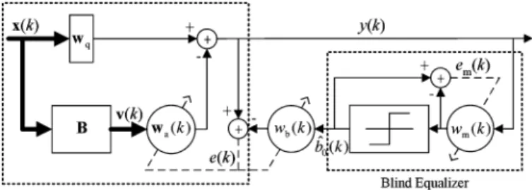
Fig. 1. Block diagram of adaptive DF-GSC.
white and Gaussian with a variance of . As shown in (2), we have decomposed the received signal into three components: desired signal, interference, and noise. For communication applications, corresponds to the channel output which is a convolution of the channel response and the original transmitted symbol sequence. For simplicity, we only con-sider quadrature phase-shift keying (QPSK) modulation and flat-fading channel environments in this paper. Thus, we can
have , where is the channel response
and is the desired transmitted symbol. The channel response can be further expressed as , where is the amplitude response and is the phase response.
B. GSC Implementation
The narrowband beamformer output at time instant , i.e.,
, can be expressed as , where is the
weight vector, and the superscript denotes the Hermi-tian operation. The LCMV beamformer determines by minimizing the interference and noise output power under appropriate linear weight constraints, which is given as
(3)
where is the input
correlation matrix of interference-plus-noise, is an
constraint matrix, and is a 1 response vector, with being the number of constraints. Several different philosophies can be employed for choosing the constraint matrix and the response vector [18]. In many communication applications, the correla-tion matrix is usually not available. Consequently, the
input correlation matrix in the receiver
is used instead. The optimization problem then becomes (4) which is called the linearly constrained minimum power (LCMP) criterion [18]. The following development will be based on this workable criterion. It is not difficult to see that the optimum weight vectors solved by (3) and (4) yield the same gain and the same output spectrum when the signal is perfectly matched and the distortionless constraint is imposed [18].
The GSC is an alternative formulation of the LCMV/LCMP beamformer. It has been shown that the GSC can convert the constrained optimization in (3) or (4) into an unconstrained one [7]. The structure of the conventional GSC is illustrated in the left part of Fig. 1. As shown in the figure, the upper path includes the quiescent signal matched filter . The lower path includes the blocking matrix and the interference cancelling filter .
Ideally, the span of is in the null space of . From the left part of Fig. 1, we can obtain the output of the GSC expressed as
(5)
where is of dimension 1, of dimension ,
and of dimension 1. Using the constraint in (4), we can solve as
(6) Let denote a cost function of MSE. The con-strained optimization problem in (4) can then be rewritten as the following unconstrained optimization problem
(7) Then, we can find the optimum as
(8)
Let . The minimum mean-squared
error (MMSE) for (7), denoted as , is calculated as
(9) It is simple to see that is just the minimum GSC output power, denoted as . When the number of antennas is larger than the number of interfering sources, i.e., the degrees of freedom (DOFs) are high enough, and the distortionless constraint is set to the desired signal’s DOA, all interference tends to be cancelled in the GSC output [6]. The MMSE will then be dominated by the output desired signal power.
(10) where and denote the desired signal power (variance) in the beamfomer input and output, respectively.
The output signal-to-interference-plus-noise ratio (SINR) is a widely accepted performance measure for beamforming. The optimum SINR can be written as
(11) For the conventional GSC, the numerator of the SINR expres-sion is just the power of the desired signal in the output, as shown in (10), and the denominator of the SINR is the power of the in-terference-plus-noise in the output, which can be found to be
(12) The general expression for the optimum SINR can then be sum-marized as
(13)
Since and are known a priori, can be calculated of-fline using (6). The optimum , however, depends on the input correlation matrix which cannot be known in advance. A simple alternative to find the optimum is to use an adaptive training method. The LMS algorithm, being one of the stochastic gra-dient methods, is known to be a simple yet effective adaptive al-gorithm [24]. Using the cost function in (7), we can calculate the stochastic gradient with respect to . The LMS update equa-tion for is written as
(14) where is the estimate of at the th snapshot,
is the filter input vector (the output vector from the blocking matrix), is the step size controlling the convergence rate, and is an error signal between the desired and actual outputs. For GSC applications, we have .
As mentioned, the conventional GSC is sensitive to a DOA mismatch which can easily occur in practical circumstances. Also, as seen from (14), the update term of the LMS algorithm involves , which will approach the output desired signal ideally. This indicates that the stochastic gradient in (14), i.e., , will not be close to zero even for optimum weights. As a result, the excess MSE induced by the LMS al-gorithm will be large. It has been shown that the excess MSE is roughly proportional to [24], where is the MMSE value in (9). To reduce the excess MSE, we then have to use a small step size and this slows the convergence of the conven-tional LMS-based adaptive GSC.
III. DECISIONFEEDBACKGSC (DF-GSC)
In this section, we propose a new DF scheme to improve the robustness and performance of the conventional GSC. Fig. 1 shows the whole structure of the proposed DF-GSC. The idea is to introduce a blind equalizer and a feedback filter to modify the GSC output , which is then used as the error signal in the LMS adaptation. The purpose of the blind equalizer is to equalize the channel and the DOA mismatch effect, and the feedback filter is to cancel any desired signal component in the LMS error signal. Due to the scenario we considered, we only need one weight for the equalizer and one weight for the feed-back filter. Note that the blind equalizer and the feedfeed-back filter are trained by different error signals. The equalizer is trained by the error signal between the output and input signals of the decision device while the feedback filter is trained by the error signal between the GSC and the feedback filter outputs. The ad-vantage of this structure is that there will be no coupling effect between these two filters. The blind equalizer can recover with a phase ambiguity and we will show that this is sufficient for our use. Although any other blind equalization algorithms can be applied, we found that they may not be more effective for the scenario considered here. The optimum weight for the blind equalizer is obtained by minimizing an MSE criterion shown here
where , with being the detected symbol and being the equalizer tap weight. Taking the sto-chastic gradient of in (15) and applying the LMS algorithm, we can obtain the update equation for as
(16) where is the step size controlling the convergence behavior of . It can be easily shown that the tap weight in (16) can equalize the channel effect up to a phase ambiguity of , where 1, 2, 3 for QPSK modulation. Since our purpose is just to cancel the desired signal component in the GSC output, knowledge of the exact transmitted symbol is not required. We now state the reason: Let denote the feedback tap weight and denote the optimum choice for it. We assume that and the decision is correct, i.e., . Then, let the decision have a phase ambiguity of , i.e., . It is simple to see that if we make , the output of the feedback filter will remain exactly the same.
With the proposed feedback structure, the cost function for the DF-GSC is changed to
(17)
As aforementioned, may have a phase ambiguity with re-spect to , but this will not affect the final result. For con-venience, we simply assume that the decision is correct, i.e., in the following analysis. Similarly, the channel effect does not have any impact in our analysis and is as-sumed to be . We may write the detected desired signal
as . With the point
distortion-less constraint, the minimization of the cost function in (17) can be written as (18) in which we let (19) (20) and (21) where denotes a zero vector with dimension 1. It is simple to see that is the same as that in the conventional GSC. Taking the derivative of the cost function with respect to
and setting the result to zero, we can obtain the optimum
(22) Thus,
(23) Utilizing the special structure of , we can decompose back into the two weights
(24) (25) With , , , and the result in (9), the minimum of (17) (which is not the minimum output power in this case) for the DF-GSC becomes
(26) We can see that the desired signal component is totally excluded from the MMSE expression for the DF-GSC and the resultant MMSE can thus be small. From the equations given above, we find three notable features of the DF-GSC.
• The expression of in (24) is the same as that in the conventional GSC.
• The effect of the additional feedback tap weight is only to reduce the minimum value of the cost function. Since and remain the same, the minimum output power is not affected.
• From (25), the output of the optimum feedback filter can be shown to equal , which is exactly the desired signal component in the output upon ideal error-free conditions.
Equation (13) is still valid for expressing the optimum output SINR for the DF-GSC, where used is the minimum output power as given in (9). Therefore, the optimum GSC performance is not enhanced by the DF operation. However, when there is a DOA mismatch or the LMS is used to estimate those optimum weights, the performance can be greatly im-proved by the DF structure. This will be elaborated in the next two sections. Similarly, the LMS update equations for the tap weights of the DF-GSC can be written as
(27) (28) where is the step size for , is the step size for ,
is the filter input vector, and .
Un-like the conventional GSC, the steady-state will exclude the desired signal component and hence can be quite small. It is where the improvement of the DF-GSC stems from. The deriva-tions given above are based on the assumption that the decision is correct. Actually, decision errors occur sometimes. In gen-eral, they can be seen as some sparse noise added to the error
signal . If the error rate is low, this will only increase the MSE slightly. We will show by simulation that even when the decision error rate is high [signal-to-noise ratio (SNR) is low], the overall performance of the DF-GSC is still better than (or at least the same as) that of the conventional GSC.
IV. DOA MISMATCHANALYSIS
A. Mismatch Signal Model
From Section II, we have defined the expression of the signal steering vector under perfectly matched conditions. If there is a mismatch between the actual and presumed desired signal’s DOA, i.e., , where is the estimated DOA and is the mismatch value, we may rewrite the steering vector as
(29) with . With modern DOA estimation methods [4], [18], is generally small (if existed). Thus, we can have
(30) We may approximate the mismatch steering vector as
(31) in which each element in the mismatch steering vector is composed of an ordinary steering term multiplied by another mismatch steering term. Without loss of generality, we let the system be presteered, i.e., is adjusted to 0 . The mismatch steering vector can then be simplified to
(32) We use (32) as the desired signal’s steering vector for the fol-lowing analysis. Then, , being equal to ,
be-comes .
B. Mismatch Analysis With GSC and DF-GSC
With an estimation error of the desired signal’s DOA, is not matched to the desired signal’s steering vector, and cannot obstruct the desired signal entering the input of the interference cancelling filter. If there are enough DOFs, the filter will cancel the desired signal from the quiescent filter output. The so-called signal cancellation occurs. In the case of the conventional GSC, even with the optimum weight vector (under distortionless con-straint), it does not provide the ability to maximize the SINR anymore [8]. The expression of the optimum output SINR for the conventional GSC is again the same as given in (13), but
now changes. The output desired signal power in the con-ventional GSC becomes
(33) which is different from (10) because is not zero now. The actual amount of signal attenuation depends upon the power of the signal and the amount of error [28]. The minimum output power for calculating the optimum output SINR of the conventional GSC in mismatch is the same as (9).
On the other hand, we can show that the signal cancellation phenomenon is avoided in the DF-GSC. Since a correlation ex-ists between the two signal paths in the GSC structure whenever a mismatch exists, the optimum solutions for and in the DF-GSC are coupled together. From (23), we have
(34) with
(35) and
(36)
where , which is the correlation between
the blocking matrix output and the decision . By using the inversion identity for subblock matrices [29], we can find the inverse of and so in (34). For reference, we give the inversion form used here as
(37)
where is the Schur complement of .
After some manipulation, we have
(38) and thus the coupled and can be written as
(39) (40) The MMSE of the DF-GSC with mismatch can then be solved to be
It is equivalent to say that the error signal contains no desired signal. This result can also be seen as the fact that from (40), the output of the optimum feedback filter is equal to , which is again exactly the output de-sired signal. It makes the interference cancelling filter have no means to cancel the desired signal in the GSC output. Here, we notice that the optimum weights are modified. From (24) and (39), we observe that the only difference between the two solu-tions of is that the correlation matrix involved is changed from to . The expression in (39) can be explained as the solution of the originally unreachable LCMV optimization problem given in (3), or its GSC implementation as
(42) As said previously, this criterion is generally not workable in practical situations for wireless communications because is not available in the receiver. However, the proposed method can equivalently minimize this criterion. This is where the robustness comes from and why signal cancellation can be avoided.
Although the optimum interference cancelling filter is changed, the expression in (13) is still valid for calculating the optimum output SINR for the DF-GSC. The power of the desired signal in the output is the same as (33), but for the DF-GSC in mismatch, the minimum output power should be calculated as
(43) In Section VI, we will use simulation results to depict the output SINR difference between the conventional GSC and DF-GSC.
C. A Blind Approach for DF-GSC With Mismatch
In the LMS-based adaptive implementation, a remaining problem is how to acquire correct decisions initially whenever a DOA mismatch occurs. In this situation, the desired signal may be too weak to initiate the blind equalizer. A straightforward method is to use training. From experiments, we find that the number of training snapshots needed is usually small for both the feedback filter and equalizer. An alternative method is to add derivative constraints, which is a classic approach for providing robustness against mismatch. With suitably chosen derivative constraints, the DF-GSC can exclude the use of training snapshots and acquire correct decisions chiefly. The disadvantage of this approach is that the DOFs are reduced and so the interference and noise suppression ability degrades.
We now develop a scheme which can let the DF-GSC skip the use of training symbols in the initial phase and reach the good SINR performance through adaptation. The idea is to use enough number of derivative constraints for the DF-GSC ini-tially and then release the constraints gradually. The iniini-tially broadened main beam can tolerate a certain amount of DOA mismatch value and ensure that there is enough desired signal strength in the quiescent filter output. Then, the equalizer can effectively converge without training. After convergence, the DF-GSC may release the constraints one by one. This incre-ment in the DOFs makes the beamformer have the opportunity to strengthen the interference and noise suppression capability.
The detailed operation of this blind approach is stated as fol-lows. For illustration, we assume that the number of point-plus-derivative constraints is changed from to , and so the
DOFs increase from to . We denote the
blocking matrix, the quiescent signal matched filter, and the in-terference cancelling filter when the DOFs are as , and . With 0 presteering, can be calculated beforehand with any DOFs and can be arbitrarily chosen ac-cording to the subspace constraints. To add the blocking matrix only one column and increase the DOFs one at a time, we need the following preliminaries.
Initialization:
1) Prepare the projection matrix for as
(44) 2) Calculate the projection of the ready to throw away column of the derivative
constraint in onto the subspace spanned
by columns of as
(45) 3) Prepare a vector holding the difference between the new and old quiescent weight vector
(46) add a zero tap weight to form the new in-terference cancelling filter
(47)
and define a sequence with elements
monotonically increasing from 0 to 1,
e.g., , where is the
sequence length. We may use a simple
se-quence , with
.
Note that the length indicates the number of snapshots during the transition. The longer the length is, the smoother the transition becomes. As a rule of thumb, it may be proportional to the average time constant of the LMS algorithm, which is ap-proximated as [24]
(48) where is the average eigenvalue for the underlying corre-lation matrix. Since the transient response settles in about four times of this average time constant, the length of can be chosen to be somewhat larger than , e.g., . It guaran-tees that there is enough smoothness and no waste of snapshots during transition. After the initialization, the DF-GSC can adopt the new adaptation settings as stated.
Transition:
1) Estimate the new weight vector iteratively according to the new blocking matrix and quiescent weight vector as
(49) (50)
with acting as the th element in the
sequence used for the th snapshot.
2) Repeat step 1) until .
Using the above procedure, the DF-GSC can skip the use of training without degrading the SINR performance eventually.
V. CONVERGENCEANALYSIS
In this section, we give the convergence analysis for both the adaptive GSC and adaptive DF-GSC.
A. MSE in Steady State
Let the MSE in steady state of the LMS algorithm be denoted
as . Then
(51) where is the MMSE solved by Wiener equations and is the excess MSE caused by the LMS adaptation. Also define the weight-error vector as
(52) Using the the direct averaging method [24], we have
(53) where denotes the error signal produced with the op-timum weights. Define the correlation matrix of the weight-error vector as
(54) Invoking the independence assumption [24], we can obtain the recursive relation of as
(55) Under this premise, the excess MSE is written as
(56) where is the trace of the matrix in brackets. As , the excess MSE is given by
(57)
where indicates the th eigenvalue of .
Hence, the excess MSE is roughly proportional to the resultant MMSE and the step size used.
B. SINR in Steady State
The output SINR in steady state is used as the performance measure for the adaptive GSC and adaptive DF-GSC. The tran-sient SINR of both schemes can be written as
(58) Without mismatch, as , the numerator of the SINR ex-pression is the same as given previously in (10); however, the denominator of the SINR is changed to
(59) where specifically denotes the minimum output power as given in (9). Thus, the steady-state SINR with the LMS algo-rithm can be summarized as
(60) Equation (60) shows how affects the steady-state SINR. The smaller the excess MSE value is, the larger the steady-state SINR becomes. From (57), we can see that is propor-tional to . For the conventional GSC and DF-GSC, their MMSEs are shown in (9) and (26), respectively. It is apparent that the MMSE of the DF-GSC is much smaller. As a result, with the same step size, the output SINR of the adaptive DF-GSC is higher than that of the conventional adaptive GSC.
In the DOA mismatch case, we define as the excess MSE of the leaky desired signal component present in the lower path. The corresponding correlation matrix of this component is
where . Using (57), we can have
(61) since only one eigenvalue of is nonzero. The expres-sion of the steady-state output SINR with mismatch is then slightly modified as
(62) In (62), for both the conventional GSC and DF-GSC and for the DF-GSC should be changed to (33) and (43), re-spectively. Another well-known adaptive algorithm is the nor-malized LMS (NLMS) algorithm. It has the advantages of better step size control and faster convergence. However, its computa-tional complexity is also higher. Though the convergence be-havior of the NLMS algorithm is similar to that of the LMS al-gorithm, the theoretical analysis is more involved.
Fig. 2. Learning curves for GSC and DF-GSC with same step size.
VI. SIMULATIONS
Computer simulations are conducted to verify our an-alytic results and demonstrate the effectiveness of the proposed algorithm. In all cases, we assume a ULA with spaced half a wavelength apart. The transmitted symbols are randomly generated from . We consider one desired source and three uncorre-lated interfering sources coming from 0 , 20 , 50 and , respectively. The total interference-to-noise ratio (INR) is 60 dB, with 20 dB per interference. The SNR is 0 dB and the step size for is 1 , unless specified otherwise. The step size for is fixed at 0.01. In all figures, 200 simulation runs are averaged to obtain each simulated result.
A. Exactly Known Desired Signal’s DOA
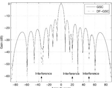
In this set of simulations, only the point distortionless con-straint is considered. The flat-fading channel coefficients for those signal vectors are independently and randomly generated, and remain unchanged in each simulation run. For comparison purpose, all these coefficients are scaled to let the average INR and SNR stick to the requirements. Since the desired signal’s DOA is exactly known (no mismatch), no training is needed for the DF-GSC. First, we use the same step size for both the con-ventional adaptive GSC and adaptive DF-GSC and observe their convergence and steady-state SINR. Fig. 2 shows the learning curves of both algorithms. Also shown is the optimum SINR value calculated with the Wiener solution. From Fig. 2, we see that the adaptive DF-GSC can achieve higher SINR than the conventional adaptive GSC, and both algorithms are compa-rable in convergence rate. As expected, the DF-GSC can ap-proach the optimum SINR much closely, which means that the effect of the excess MSE induced by the LMS algorithm is small. Fig. 3 reveals the beam patterns of both adaptive schemes after 200 snapshots. It is clear that the adaptive DF-GSC per-forms better than the adaptive GSC in nulling the interference. The difference between the two schemes is almost 10 dB for each interfering source.
We then fix a target SINR, i.e., 11 dB, and choose suitable step sizes for both schemes ( and
Fig. 3. Beam patterns of GSC and DF-GSC in Fig. 2 after 200 snapshots.
Fig. 4. Learning curves for GSC and DF-GSC with same SINR target.
for the conventional adaptive GSC and the adaptive DF-GSC, respectively). It is to compare the convergence rate of both al-gorithms. Fig. 4 demonstrates the results. As we can see, the DF-GSC converges around 150 snapshots while the GSC con-verges around 350 snapshots. The DF-GSC concon-verges much faster.
Next, we present the steady-state SINR achievable by the con-ventional adaptive GSC and the adaptive DF-GSC under dif-ferent SNR environments. Fig. 5 shows the results. We see that the achievable SINR for the DF-GSC is proportional to the SNR and that for the GSC is saturated when the SNR is high. The per-formance gap becomes significant in high SNR regions.
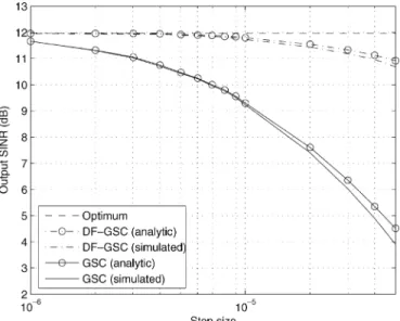
Afterward, we show the SINR performance with different step sizes used for in the LMS algorithm. Fig. 6 gives the simulation results. It is clear that the larger the step size, the lower the SINR performance. However, we notice that the SINR degradation due to large step sizes in the adaptive DF-GSC is much smaller than that in the conventional adaptive GSC. For this reason, the DF-GSC can work with a large step size to achieve fast convergence, which is very useful in time-varying environments. From all these figures described earlier, we can
Fig. 5. Steady-state SINR performance in different SNR environments.
Fig. 6. Steady-state SINR performance with different step sizes.
conclude that when the LMS algorithm is used for adaptation, the DF-GSC can achieve higher SINR for the same convergence rate or faster convergence rate for the same SINR. We also see that our theoretical SINR analysis is quite accurate.
B. Desired Signal’s DOA Mismatch
Here, a scenario with a DOA mismatch is considered. We as-sume that there is a 2 difference between the estimated and ac-tual desired signal’s DOA. Here, the step size for is chosen to be 5 for fast convergence. Fig. 7 shows the learning curves for the conventional adaptive GSC with different con-straint settings. From the figure, with the point concon-straint only, the SINR will eventually degrade to around . It means that the desired signal is almost entirely cancelled out by the interference cancelling filter. Again, in the same figure, we see that with the additional first-order derivative constraint, the con-ventional GSC exhibits some robustness against the mismatch, but the signal cancellation still occurs. The steady-state SINR for this case is about 2 dB.
Fig. 7. Learning curves for GSC with DOA mismatch utilizing point (pt) constraint only and point and first-order derivative (pt & 1d) constraints.
Fig. 8. Learning curves for DF-GSC with DOA mismatch utilizing point (pt) constraint only and point and first-order derivative (pt & 1d) constraints.
We repeat the same experiment described previously with the adaptive DF-GSC and show the results in Fig. 8. Here, the first 50 snapshots are used as training for the scenario with the point constraint only and no training is required for the scenario with the point and first-order derivative constraints. We see that these schemes with the two different constraint settings achieve SINR about 9 and 7.5 dB, respectively. No signal cancellation seems to occur. Adding the additional constraint lowers the SINR for the DF-GSC because DOFs are reduced. We conclude that the proposed algorithm can provide notable robustness for the GSC structure. From Figs. 7 and 8, we also notice that the simulated curves match the analytic ones well.
From the experiment in Fig. 8, we observe that for the 2 DOA mismatch, the point and first-order derivative constraints are enough for the adaptive DF-GSC to bypass the training pe-riod. However, the output SINR lessens. To keep the blind na-ture for the DF-GSC strucna-ture and achieve higher SINR, we may adopt the approach described in Section IV-C. Fig. 9 shows the
Fig. 9. Learning curves for DF-GSC with transition from point and first-order derivative (pt & 1d) constraints to point (pt) constraint only.
Fig. 10. Steady-state SINR performance for DF-GSC and other robust adaptive beamforming approaches in different SNR environments.
learning curve of the blind approach for our mismatch example. The DF-GSC works with the point and first-order derivative constraints at the beginning. After 100 snapshots, it smoothly switches to use the point constraint only. The duration of tran-sition is set to 80 snapshots (about ). We see that the DF-GSC converges after about 200 snapshots without using any training snapshots.
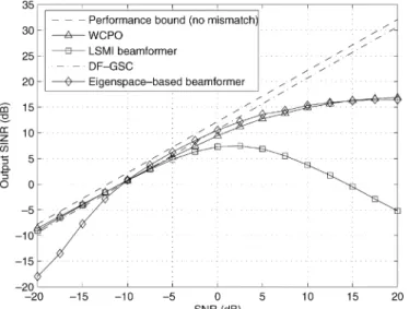
Finally, we compare the performance for the DF-GSC with some well-known robust adaptive beamforming schemes against the DOA mismatch. The step size for is chosen to be 1 here. The loaded sample matrix inversion (LSMI) al-gorithm, WCPO alal-gorithm, and eigenspace-based beamformer are chosen for comparison. The number of training snapshots required by these robust methods is set to 100, which is large enough for providing good performance [22]. The diagonal loading factor for the LSMI is taken to be , where is the noise power in a single antenna element. The parameter in the WCPO algorithm is selected to provide nearly the optimum performance [22]. Fig. 10 shows the simulation results. From the figure, we observe that the performance of the DF-GSC is
almost the same as the WCPO and LSMI algorithms in low SNR regions, but the DF-GSC outperforms all other algorithms in middle to high SNR regions. Based on the results, we conclude that the DF-GSC is the only robust algorithm whose performance is consistently close to the optimum from low to high SNR regions.
VII. CONCLUSION
In this paper, a new LMS-based adaptive DF-GSC has been proposed. The DF-GSC introduces a blind equalizer and a feed-back filter in the GSC structure. We theoretically show that the optimum interference cancelling filters for both the DF-GSC and conventional GSC are the same with perfectly known DOA. Robustness analysis for the two schemes with a DOA mismatch is also given. We derive the Wiener solution for the interfer-ence cancelling filter when the DF-GSC is in mismatch and show that the signal cancellation phenomenon can be avoided. On the other hand, when the optimum weights are estimated by the LMS algorithm, the DF-GSC gives significantly better results than that of the conventional GSC. We have examined the convergence behavior of the conventional adaptive GSC and the proposed adaptive DF-GSC under perfectly matched and mismatched DOA scenarios. Simulation results verify that the DF-GSC can achieve higher SINR value for the same conver-gence rate or faster converconver-gence for the same SINR, and the DF-GSC can keep the high SINR performance even in mis-match. In this paper, we confine ourselves in the flat-fading channel and QPSK modulation environments. For general mul-tipath fading channels, the equalizer and the feedback filter must be extended to tap-delay-line structures. Also, for high-order signal constellation modulation such as quadrature amplitude modulation (QAM), other sophisticated blind equalization al-gorithms may be required. Research in these topics is now un-derway.
REFERENCES
[1] R. A. Monzingo and T. W. Miller, Introduction to Adaptive
Ar-rays. New York: Wiley, 1980.
[2] B. D. Van Veen and K. M. Buckley, “Beamforming: A versatile approach to spatial filtering,” IEEE Acoust., Speech, Signal Process. Mag., vol. 5, pp. 4–24, Apr. 1988.
[3] T. K. Sarkar, M. C. Wicks, M. S. Palma, and R. J. Bonneau, Smart
An-tennas. New York: Wiley-IEEE, 2003.
[4] L. C. Godara, “Applications of antenna arrays to mobile communica-tions, Part II: Beam-forming and direction-of-arrival consideracommunica-tions,”
Proc. IEEE, vol. 85, pp. 1195–1245, Aug. 1997.
[5] Adaptive Antennas for Wireless Communications, G. V. Tsoulos, Ed.,
Wiley-IEEE, New York, 2001.
[6] O. L. Frost III, “An algorithm for linearly constrained adaptive array processing,” Proc. IEEE, vol. 60, pp. 926–935, Aug. 1972.
[7] L. J. Griffiths and C. W. Jim, “Alternative approach to linear constrained adaptive beamforming,” IEEE Trans. Antennas Propag., vol. AP-30, pp. 27–34, Jan. 1982.
[8] B. Widrow, K. M. Duvall, R. P. Gooch, and W. C. Newman, “Signal cancellation phenomena in adaptive antennas: Causes and curse,” IEEE
Trans. Antennas Propag., vol. AP-30, pp. 469–478, May 1982.
[9] A. B. Gershman, “Robust adaptive beamforming in sensor arrays,” Int.
J. Electron. Commun., vol. 53, pp. 305–314, Dec. 1999.
[10] T. Takao and C. S. Boon, “Importance of the exclusion of the desired signal from the control of a generalized sidelobe canceller,” Proc. Inst.
Elect. Eng., pt. F, vol. 139, pp. 256–272, Aug. 1992.
[11] D. D. Feldman and L. J. Griffiths, “A projection approach to robust adap-tive beamforming,” IEEE Trans. Signal Process., vol. 42, pp. 867–876, Apr. 1994.
[12] D. D. Feldman, “An analysis of the projection method for robust adaptive beamforming,” IEEE Trans. Antennas Propag., vol. 44, pp. 1023–1030, Jul. 1996.
[13] K. C. Huarng and C. C. Yeh, “Performance analysis of derivative constraint adaptive arrays with pointing errors,” IEEE Trans. Antennas
Propag., vol. 40, pp. 975–981, Aug. 1992.
[14] S. Park and T. K. Sarkar, “Prevention of signal cancellation in adaptive nulling problem,” Digital Signal Process., vol. 8, no. 2, pp. 95–102, Apr. 1998.
[15] Y. Chu and W. H. Fang, “A novel wavelet-based generalized sidelobe canceller,” IEEE Trans. Antennas Propag., vol. 47, pp. 1485–1494, Sep. 1999.
[16] H. Cox, R. M. Zeskind, and M. H. Owen, “Robust adaptive beam-forming,” IEEE Trans. Signal Process., vol. 35, pp. 1365–1376, Oct. 1987.
[17] J. R. Guerci, “Theory and application of covariance matrix tapers for robust adaptive beamforming,” IEEE Trans. Signal Process., vol. 47, pp. 977–985, Apr. 1999.
[18] H. L. Van Trees, Detection, Estimation, and Modulation Theory:
Op-timum Array Processing. New York: Wiley, 2002, pt. 4.
[19] M. H. Er, “A unified approach to the design of robust narrow-band an-tenna array processors,” IEEE Trans. Anan-tennas Propag., vol. 38, pp. 17–23, Jan. 1990.
[20] A. Cantoni, X. G. Lin, and K. L. Teo, “A new approach to the optimiza-tion of robust antenna array processors,” IEEE Trans. Antennas Propag., vol. 41, pp. 403–411, Apr. 1993.
[21] J. H. Lee and Y. T. Lee, “Robust adaptive array beamforming for cyclo-stationary signals under cycle frequency error,” IEEE Trans. Antennas
Propag., vol. 47, pp. 233–241, Feb. 1999.
[22] S. A. Vorobyov, A. B. Gershman, and Z. Q. Luo, “Robust adaptive beam-forming using worst-case performance optimization: A solution to the signal mismatch problem,” IEEE Trans. Signal Process., vol. 51, pp. 313–324, Feb. 2003.
[23] S. Shahbazpanahi, A. B. Gershman, Z. Q. Luo, and K. M. Wong, “Robust adaptive beamforming for general-rank signal models,” IEEE
Trans. Signal Process., vol. 51, pp. 2257–2269, Sep. 2003.
[24] S. Haykin, Adaptive Filter Theory, 3-rd ed. Englewood Cliffs, NJ: Prentice-Hall, 1996.
[25] T. K. Sarkar, E. Arvas, and S. M. Rao, “Application of FFT and the conju-gate gradient method for the solution of electromagnetic radiation from electrically large and small conducting bodies,” IEEE Trans. Antennas
Propag., vol. AP-34, pp. 635–640, May 1986.
[26] T. K. Sarkar and N. Sangruji, “An adaptive nulling system for a narrow-band signal with a look-direction constraint utilizing the conjugate gra-dient method,” IEEE Trans. Antennas Propag., vol. 37, pp. 940–944, Jul. 1989.
[27] T. K. Sarkar, J. Koh, R. Adve, R. A. Schneible, M. C. Wicks, S. Choi, and M. S. Palma, “A pragmatic approach to adaptive antennas,” IEEE
Antennas Propag. Mag., vol. 42, pp. 39–55, Apr. 2000.
[28] H. Cox, “Resolving power and sensitivity to mismatch of optimum array processors,” J. Acoust. Soc. Amer., vol. ASSP–54, pp. 771–785, Sep. 1973.
[29] G. H. Golub and C. F. Van Loan, Matrix Computation, 3rd ed. Balti-more, MD: The Johns Hopkins Univ. Press, 1996.
Yinman Lee received the B.Eng. degree in
com-munication engineering from National Chiao Tung University, Hsinchu, Taiwan, R.O.C., in 1997, and the M.Phil. degree in information engineering from the Chinese University of Hong Kong, Shatin, Hong Kong, in 1999.
He is currently working toward the Ph.D. degree in the Department of Communication Engineering, National Chiao Tung University. His research in-terests include wireless communications, adaptive signal processing, and space-time processing.
Wen-Rong Wu received the B.S. degree in
mechan-ical engineering from Tatung Institute of Technology, Taiwan, R.O.C., in 1980. He received the M.S. degree in mechanical engineering, the M.S. degree in elec-trical engineering, and the Ph.D. degree in elecelec-trical engineering from the State University of New York, Buffalo, in 1985, 1986, and 1989, respectively.
Since August 1989, he has been a faculty member with the Department of Communication Engineering, National Chiao Tung University, Taiwan, R.O.C. His research interests include statistical signal processing and digital communications.