Contributed Paper
Manuscript received October 19, 2004 0098 3063/05/$20.00 © 2005 IEEE
A Robust Digital Image Stabilization Technique Based
on Inverse Triangle Method and Background Detection
Sheng-Che Hsu, Sheng-Fu Liang, and Chin-Teng Lin
Abstract — In this paper, a novel robust digital imagestabilization (DIS) technique is proposed to stably remove the unwanted shaking phenomena in the image sequences captured by hand-held camcorders without affecting moving objects in the image sequence and intentional motion of panning condition, etc. It consists of a motion estimation unit and a motion compensation unit. To increase the robustness in adverse image conditions, an inverse triangle method is proposed to extract reliable motion vectors in plain images which are lack of features or contain large low-contrast area, etc., and a background evaluation model is developed to deal with irregular images which contain large moving objects, etc. In the motion compensation unit, a CMV estimation method with an inner feedback-loop integrator is proposed to stably remove the unwanted shaking phenomena without losing the effective area of the image in panning condition. We also propose a smoothness index (SI) to quantitatively evaluate the performances of different image stabilization methods. The experimental results are on-line available to demonstrate the remarkable performance of the proposed DIS technique.1,2
Index Terms — Background-Based Evaluation, Digital Image Stabilizer (DIS), Inverse Triangle Method, Representative Point Matching (RPM), Smoothness Index (SI).
I. INTRODUCTION
Digital video sequences acquired by compact and lightweight video cameras are usually affected by undesired motion produced by unstable camera holding or platform moving. The unwanted positional fluctuations of the video sequence will affect the visual quality and impede the subsequent processes for various applications such as motion coding, video compression, feature tracking, etc. The challenge of image stabilization systems is how to compensate the unwanted shacking of the camera without affecting moving objects in the image sequence and intentional motion of panning condition.
The image stabilization systems can be classified into three major types: the electronic, the optical, and the digital stabilizers. The electronic image stabilizer (EIS) stabilizes the
1 Sheng-Che Hsu is with Electrical and Control Engineering Department, National Chiao-Tung University, Hsin-Chu, Taiwan. He is also with Ta-Hwa Institute of Technology.
Sheng-Fu Liang and Chin-Teng Lin are both with Brain Research Center, University System of Taiwan and also with Electrical and Control Engineering Department, National Chiao-Tung University, Hsin-Chu, Taiwan. (Corresponding Author: Chin-Teng Lin (e-mail): [email protected]).
2 This work was supported by Ministry of Education, Taiwan, under Grant EX-91-E-FA06-4-4
image sequence by employing motion sensors to detect the camera movement for compensation. The optical image stabilizer (OIS) employs a prism assembly that moves opposite the shaking of camera for stabilization [1, 2]. Because both EIS and OIS are hardware dependant, the applications are restricted to device built-in on-line process. The digital image stabilization (DIS) is the process of removing the undesired motion effects to generate a compensated image sequence by using digital image processing techniques without any mechanical devices such as gyro sensors or fluid prism [4]. The major advantages of DIS are (1) not restriction of on/off-line applications, and (2) suitable for miniature hardware implementation (since the mechanical device is not required for compensation) [3]. The DIS can be performed either as post-processing after the video sequence was acquired, or in real-time during the acquisition process, depending on the applications. Archive films with undesired shaking effects require post-processing for the video sequences while camcorders require real-time compensation process.
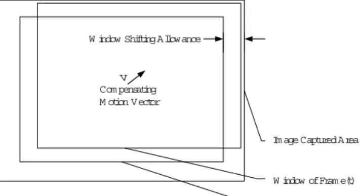
The DIS system is generally composed of two processing units: the motion estimation unit and the motion compensation unit. The purpose of motion estimation unit is to estimate the reliable global camera movement through the acquired image sequence. Following the motion estimation, the motion compensation unit generates the compensating motion vector and shifts the current picking window according to the compensating motion vector to obtain a smoother image sequence. Fig. 1 shows the motion compensation schematics. The window of frame(t-1) is the previous compensated image. The compensating motion vector v is generated by the DIS technique according to the global motion vector between two consecutive images. The position of picking window on the frame(t) is according to the compensating motion vector v to minimize the shaking effect.
Com pensating M otion V ector W indow Shifting Allow ance
W indow of Fram e(t-1) W indow of Fram e(t) Im age Captured A rea v
Various algorithms had been developed to estimate the local motion vectors such as representative point matching (RPM) [3][8], edge pattern matching (EPM) [5-6], bit-plane matching (BPM) [4][7] and others [9-13]. The major objective of these algorithms is to reduce the computational complexity, in comparison with full-search block-matching method, without losing too much accuracy and reliability. In general, the RPM can greatly reduce the complexity of computation in comparison with the other methods. However, it is sensitive to irregular conditions such as moving objects and intentional panning, etc. [7]. Therefore, the reliability evaluation is necessary to screen the undesired motion vectors for the RPM method. In [8], a fuzzy-logic-based approach was proposed to discriminate the reliable motion vector from the local motion vectors. This method produced two discriminating signals based on some image information such as contrast, moving object, and scene changing to determine the global motion vector. However, these two signals cannot cover widely various irregular conditions such as the lack of features or containing large moving objects in the images, and it is also hard to determine an optimum threshold for discrimination in various conditions. In this paper, a reliable local motion vector extraction method is proposed to determine the global motion vectors for practical real-life applications.
In the motion compensation of DIS, accumulated motion vector estimation [5] and frame position smoothing (FPS) [15-17,21] are the two most popular approaches. The accumulated motion vector estimation needs to compromise stabilization and intentional panning preservation since the panning condition causes a steady-state lag in the motion trajectory [15,21]. The FPS accomplished the smooth reconstruction of an actual long-term camera motion by filtering out jitter components based on the concept of designing the filter with appropriated cut-off frequency [15] or adaptive fuzzy filter to continuously improve stabilization performance [21].
In this paper, a novel robust DIS technique is proposed. The background detection model is integrated with the RPM method to estimate the reliable global motion vector. The accumulated motion vector estimation combined with an integrator in the inner feedback-loop is also proposed to remove the shaking effect without losing the effective area of the images in the panning condition. Video sequences with various irregular conditions have been used for testing and the experimental results demonstrate that the proposed algorithm can perform very well in such conditions. A smoothness index
(SI) is also proposed in this paper to quantitatively evaluate the performances of different image stabilization methods.
This paper is organized as follows. Section II describes the system architecture of the DIS and the proposed motion estimation method. Section III proposes motion compensation method and the quantitative evaluation. Section IV presents the experimental results for demonstrations. Section V gives conclusions of this paper.
II. SYSTEM ARCHITECTURE OF THE DIS AND MOTION
ESTIMATION
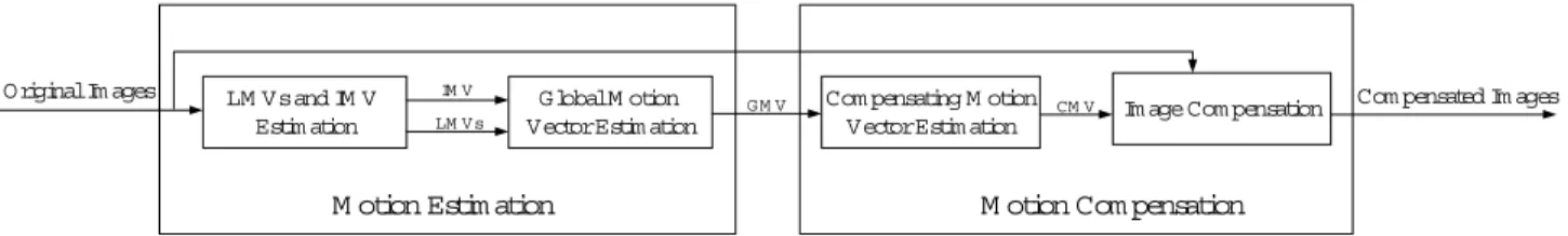
The system architecture of the proposed DIS technique is shown in Fig. 2, which includes two processing units: the motion estimation unit and the motion compensation unit. The motion estimation unit consists of three estimators: the local motion vectors (LMVs), the ill-conditioned motion vector (IMV), and the global motion vector (GMV) estimators. The motion compensation unit consists of the compensating motion vector (CMV) estimation and image compensation. The two incoming consecutive images (frame (t-1) and frame (t)) will be firstly divided into four regions as shown in Fig. 4. A LMV will be derived in each region by the representative point matching (RPM) algorithm [3][8]. The motion estimation unit also contains a reliability detection function that will generate an ill-conditioned motion vector for the irregular image conditions such as the lack of features or containing large low-contrast area, etc. The GMV estimation determines a global motion vector among LMVs, the IMV, and other pre-selected motion vectors through background-based evaluation function. Finally, the compensating motion vector (CMV) is generated according to the resultant GMV and the image sequences will be compensated based on the CMV in the motion compensation unit. The rest of this section will focus on the details of the motion estimation unit of the proposed DIS technique. The details of the proposed motion compensation unit will be presented in the next section.
A. Motion Estimation
The motion estimation unit shown in Fig. 2 contains the LMVs, IMV, and GMV estimators. As shown in Fig. 3, the LMVs and IMV estimation is to generate the LMVs and IMV for global motion vector estimation. The LMVs can be obtained from the correlation between two consecutive images by the representative point matching (RPM) algorithm [3][8][23]. The IMV can be obtained from LMVs by evaluating the corresponding confidence indices through the
Global M otion Vector Estim ation LM Vs and IM V
Estim ation
IM V LM V s
Com pensating M otion Vector Estim ation
G M V CM V Im age Com pensation
Original Im ages Com pensated Im ages
M otion Estim ation M otion Com pensation
Contributed Paper
Manuscript received October 19, 2004 0098 3063/05/$20.00 © 2005 IEEE irregular condition detection and the proposed IMV
generation algorithm.
B. RPM and Local Motion Estimation
First, the image is divided into four regions as shown in Fig. 4. Each region is further divided into 30 sub-regions (each with side of 5 rows
×
6 columns). The central pixel of each sub-region is selected as the representative point(X Yr, r) to represent the pattern of this sub-region. The correlation calculation of RPM is by 1 ( , ) ( 1, , ) ( , , ) N i r r r p r q r R p q I t X Y I t X + Y+ = =
¦
− − , (1)whereNis the number of representative points in one region,
( 1, r, r)
I t− X Y is the intensity of the representative point
(X Yr, r) at frame t− , and 1 R p qi( , ) is the correlation measure for a shift
(
p
,
q
)
between the representative points in region i at frame t− and the relative shifting points at 1frame
t
. Assuming RiMin is the minimum correlation value in region i, i.e.,, ( ( , ))
iMin i
p q
R =Min R p q , the shift vector
v
i that produces the minimum correlation value for region i represents the local motion vector of this region, i.e.( , ), for ( , )
i i iMin
v = p q R p q =R . (2)
C. Irregular Condition Detection
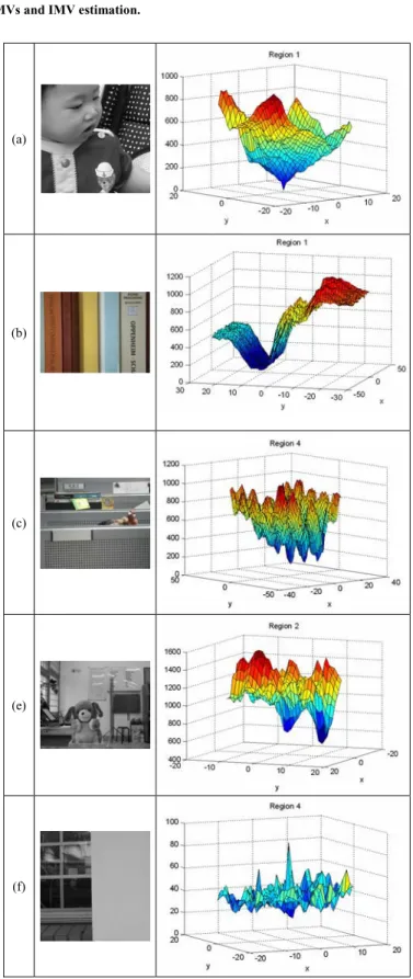
Analyzing the curves of correlation values corresponding to image sequences with various conditions, it is found that the curve of correlation values is related to the reliability of motion detection. Fig. 5 shows the various correlation curves corresponding to different sample image sequences with different conditions. Fig. 5(a) shows a normal condition that the peak is obvious in region 1. In Fig. 5(b), the curve looks like a valley in region 1; it means only one dimension of correlation data (y direction) is reliable and it lacks for feature of x (vertical) direction. Fig. 5(c) shows an example with repeated patterns and it causes multiple peaks in the curves of
(X Yr,r) (Xr p+,Yr q+)
: local motion vector( 1, 2, 3, 4)
i v i= 1 v v3 4 v 2 v
Fig. 4. Division of image for local motion vector estimation.
(a)
(b)
(c)
(e)
(f)
Fig. 5. Various correlation curves corresponding to image sequences with different conditions.
region 4. A character pattern is also viewed as repeated pattern by the RPM method. Fig. 5(d) represents moving object conditions; a bear moves from the left side to the right side of the image sequence. It causes double peaks in the curve of region 2 and the value of RiMin is larger than that in the normal images such as Fig. 5(a). The example shown in Fig. 5(e) contains a large low-contrast area on the right side of the image. Obviously, it is very hard to distinguish the peak from the correlation curves in region 4.
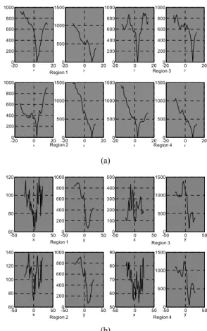
Although the curve of correlation values is related to the reliability of motion detection, it is still too complex to directly use these curves to evaluate the reliability of motion detection. In this paper, we propose a strategy that combines the minimum projections of correlation curve in x and y directions (minimum projections) and the inverse triangle method to detect the irregular conditions from each region. The mathematical expression of minimum projections can be written as
_ min( ) min ( , ) _ min( ) min ( , ) i i q i i p x p R p q y q R p q = = , (3)
where xi_ min( )p and yi_ min( )p are the minimum projections of correlation curve in x and y directions in region
i
, respectively. Fig. 6 shows the examples of minimum projections of correlation curve in x and y directions from the regular and the ill-conditioned image sequences. Fig. 6(a) shows the minimum projection of Fig. 5(a) that is regular and the determination of motion vector in each region is clear and consistent. Fig. 6(b) shows the minimum projection of Fig. 5(b) that lacks for the feature in x direction (vertical). According to Fig. 7(b) and 5(b), the value of minimum projection of correlation curve in x direction is located within a small range and the projection curve is erratic with multiple peaks which makes the determination of the minimum value very hard.In order to determine the reliability of motion vector easily, the feature extraction of reliability is performed by the proposed inverse triangle method applied into the minimum projections in x and y directions to obtain the reliability indices. Fig. 7 shows the illustration of the inverse triangle method. The concept derives from the intuitional sense that the high reliable curve for determining the LMV has a sharp and obvious peak, and no other equivalent peaks appeared in the same curve. Base on this criterion, the algorithm is designed as follows: In the first step, we find Ti_ min that represents the global minimum of the minimum projection curve in region
i
and can be calculated by (4). In the second step, we calculate S and xi S by (5), where offset is the yi altitude of the inverse triangle, n and xi n are defined as the yi numbers of S and xi S , respectively (see (6)), yi d and xi d are yi defined as the distances of two vertexes of the base of inverse triangle obtained by (7). The confidence level of x and y directions are calculated by (8). Since the condition of multiple peaks seriously degrades and affects the determination of reliability, the penalty of multiple peaks istaken into account by (8) to improve the discrimination of
reliability. The example shown in Fig. 8 is a curve with twin peaks which will get the penalty of dxi−nxi. In the third step, we determine the confidence indices of x and i y in region i i through a threshold denoted as TH . The smaller value of confidence level represents the higher reliability. In the final step, summing up the counts of reliable motion components of x and y in four regions as (9), we get Num x( )i and
( ), 1 ~ 4i
Num y i= . The follows describe the procedure:
-200 0 20 200 400 600 800 1000 x -200 0 20 500 1000 1500 y -200 0 20 200 400 600 800 1000 x -200 0 20 200 400 600 800 1000 y -200 0 20 200 400 600 800 1000 x -200 0 20 500 1000 1500 y -200 0 20 500 1000 1500 x -200 0 20 500 1000 1500 y Region 1 Region 3 Region 2 Region 4 (a) -50 0 50 60 80 100 120 x -50 0 50 0 200 400 600 800 1000 y -50 0 50 0 100 200 300 400 500 x -50 0 50 0 500 1000 1500 y -50 0 50 60 80 100 120 140 -50 0 50 0 200 400 600 800 1000 y -50 0 50 50 60 70 80 90 x -50 0 50 0 500 1000 1500 y Region 1 Region 3 Region 2 Region 4 x (b)
Fig. 6. Examples of minimum projections of correlation curve from x
and y directions in four regions. (a) Regular image sequence.
(b) Ill-conditioned image sequence.
xi d xi n offset _ min i T
Step 1.
Find global minimum _ minTi from _ min( )xi p oryi_ min( )q .
_ min min( _ min( ))
i p i
T = x p orTi_ min min( _ min( ))= q yi q . (4) Step 2.
Calculate the confidence level,xi_conf andyi_conf .
{ | _ min( ) _ min } { | _ min( ) _ min } xi i i yi i i S p x p T offset S q y q T offset = < + ⎧⎪ ⎨ = < + ⎪⎩ , (5) number of number of xi xi yi yi n S n S = ⎧⎪ ⎨ = ⎪⎩ , (6) max min max min xi P xi P xi yi q yi q yi d S S d S S = − ⎧⎪ ⎨ = − ⎪⎩ , (7) _ 2 _ 2 i xi xi i yi yi x conf d n y conf d n = − ⎧⎪ ⎨ = − ⎪⎩ . (8) Step 3.
Set the threshold,TH, for determining the reliability indices. If _xi conf < TH Then x is reliable, i
Elsex is unreliable, i End if.
If _yi conf < TH Then y is reliable, i Elsey is unreliable, i
End if. Step 4.
Calculate the numbers of
x
iandy
iin four regions. ( ) sum of ( is reliable) ( ) sum of (y is reliable) i i i i Num x x Num y = ⎧ ⎨ = ⎩ , (9) 1 ~ 4i= .D. Generation of Ill-Conditioned Motion Vector
Irregular motion vectors can be detected and excluded using minimum projection and inverse triangle method; however, image sequence with ill-condition such as lack of feature, large low-contrast area, moving object or repeated pattern, may contain fewer available MVs (most of the MVs are irregular) in four regions. Therefore, recombination of these available regular MVs is necessary to form an ill-conditioned motion vector (IMV). To solve this problem, a median function is used to extract a motion vector with respect to each direction for ill condition. The calculation to determine the IMV is described as follows in details.
Case 1. If Num x t( ( )) 4i = then
_ ( ) ( _ ( ), _ ( ), _ ( ), _ ( ), ( 1))
ill x a x b x c x d x x
V t =Med V t V t V t V t GMV t− ,
Case 2. IfNum x t( ( )) 3i = then
_ ( ) ( _ ( ), _ ( ), _ ( ))
ill x a x b x c x
V t =Med V t V t V t ,
Case 3. IfNum x t( ( )) 2i = then
_ ( ) ( _ ( ), _ ( ), ( 1))
ill x a x b x x
V t =Med V t V t GMV t− , (10)
Case 4. If Num x t( ( )) 1i = then
_ ( ) _ ( )
ill x a x
V t =V t ,
Case 5. If Num x t( ( )) 0i = then
_ ( ) ( 1)
ill x avgx
V t = ×γ GMV t− ,
whereNum x t is the number of x component of reliable ( ( ))i LMVs, Vill x_ ( )t is the x component of IMV, Va x_ ( )t , Vb x_ ( )t ,
_ ( )
c x
V t , and Vd x_ ( )t represent x components of reliable LMVs in different region, respectively, Med( ) is the function of median operation, GMV tx( −1) is the x component of last previous GMV,
t
is frame number,γ
is attenuation coefficient, 0< < . The γ 1 GMVavgx( )t can be calculated by ( ) ( 1) (1 ) ( ), 0< <1. avgx avgx x GMV t ζGMV t ζ GMV t ζ = − + − (11) Then we apply the similar process to obtain Vill y_ ( )t . Theresultant IMV is represented by _ _ ( ) ( ) ( ) ill x ill ill y V t V t V t ⎡ ⎤ = ⎢ ⎥ ⎣ ⎦. (12)
E. Global Motion Vector Estimation
The LMV in each region may represent global motion vector, moving object motion vector, or even error vector. The error vector may be caused by the ill condition or the mixture of global motion and moving object motion. Although the reliable global motion vector is essentially selected from LMVs and IMV, however, in the worst case, i.e. estimations of LMVs and IMV are all fault due to high noise image sequence, it will induce artificial shaking result due to adopt an error GMV. Therefore, if the evaluation includes the zero motion vector (ZMV), it can prevent the occurrence of this case. Similarly, for a high noise image sequence with panning, the last previous GMV will be the best choice if the estimations of LMVs and IMV are all fault. In the proposed DIS technique, the seven motion vectors including four LMVs, the IMV, the ZMV, and the last previous GMV, referred as pre-selected motion vectors ( pre MV ), are employed to estimate the GMV of the _ current frame. In general, one of LMVs is the highly probable GMV for the regular image; the IMV is the highly probable GMV for ill-conditioned image; the ZMV can prevent worse compensation result caused by the fault MVs; and the last previous GMV is useful for panning condition.
In addition, if the image sequence contains a large moving object, the determination of global motion is troublesome because the determined motion vector probably switches between background and large moving object or is totally dominated by the large moving object. In this case, it will lead to artificial shaking and cause an important challenge in DIS. In this paper, a background-based evaluation function is proposed to overcome this problem. Fig. 8 shows the areas
for background-based evaluation. Five regions are selected to evaluate the result, which are located on the surroundings of the image. The reason is that, in most cases, the foreground object is located on the center of the image, so the
surroundings of the image are the best candidates for background detection. The estimation of the GMV is calculated by the summation of absolute difference (SAD),
, , ( 1, , ) ( , , ) , 1 5, 1 7, i i B c c c X Y B SAD I t X Y I t X X Y Y i c ∈ = − − + + ≤ ≤ ≤ ≤
∑
(13)where (I t−1, , )X Y is the intensity of the point ( , )X Y at frame t-1, B is the i-th background region in the image, i
,
c c
X Y are the components of the seven pre-select motion vectors (pre MV ) in x and y directions. _ c
Eachpre MV can obtain it’s _ c SADB ci, in each region. The smaller SADB ci, represents the higher probability of the desired motion vector among theses pre-selected motion vectors. The score for eachpre MV in region _ c
i
is denoted asS , which is the order of the i c, SADB ci, value, and the higher,
i
B c
SAD indicates the higher score. The total score for each
_ c
pre MV can be obtained by 5 , 1 c i c i S S = =
∑
. (14)Five-region peer-to-peer evaluation can prevent the situation that some partial high-contrast image regions dominate the evaluation result. In this algorithm, each region
has an equal priority to determine the result. In (14), S is the c index to determine the GMV. The pre MV with the _ c smallest S is the desired GMV and it can be expressed as c GMV=pre MV , for _ i arg(min c)
c
i= S . (15)
According to these sophisticated evaluation areas, the evaluation function can detect attributed background motion vector precisely in most circumstances.
III. MOTION COMPENSATION AND EVALUATION
A. Compensating Motion Vector (CMV) Estimation The first step of motion compensation is to generate the compensating motion vectors (CMVs) for removing the undesired shaking motion but still keeping the steady motion of the image sequence. The conventional compensating motion vector estimation was given by [5]
( ) ( ( 1)) ( ( ) (1 ) ( 1))
CMV t =k CMV t− + αGMV t + −α GMV t− ,(16)
where t represents the frame number, 0< <k 1 and 0≤ ≤ . The increase in k causes the decrease in unwanted α 1 shaking effect but increase in the value of CMV, which means the effective area of images is reduced if we want to maintain the consistent image size for the whole image sequence. To illustrate this phenomenon, the motion trajectories can be calculated to analyze the problem. The motion trajectories can be obtained by 1 ( ) t ( ) o i MTraj t GMV i = =
∑
, (17) 1 ( ) t ( ( ) ( )) c i MTraj t GMV i CMV i = =∑
− , (18)where ( )MTraj t and o MTraj t are the original and the c( ) compensated motion trajectories of the image sequence at frame t.
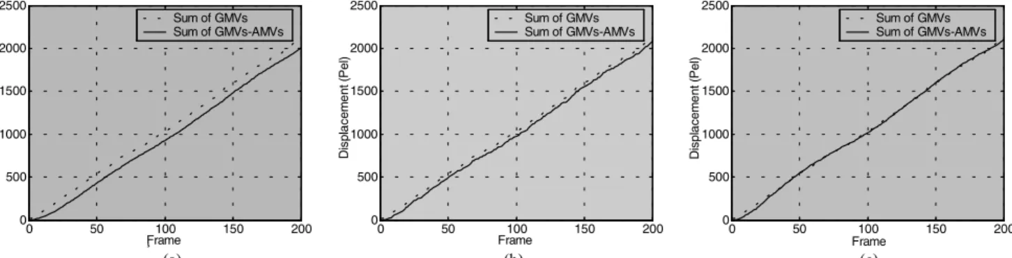
Fig. 9 shows the performance comparison of three different CMV generation methods applied to a video sequence with panning and hand shaking. There are two trajectories in each subfigure; one is the original trajectory calculated by (17) and the other one is the compensated trajectory calculated by (18). The CMVs in Fig. 9(a) are generated by the conventional method shown in (16). Obviously, MTraj t has tremendous c( )
2 4
1 5 3
50x150 pels 50x150 pels 150x50 pels 100x100 pels 150x50 pels
640x480 pels
Fig. 8. Areas for background detection and evaluation.
0 50 100 150 200 0 500 1000 1500 2000 2500 ¸Frame D isp la ce m e n t ( P e l) Sum of GMVs Sum of GMVs-AMVs 0 50 100 150 200 0 500 1000 1500 2000 2500 Frame D isp la ce m e n t ( P e l) Sum of GMVs Sum of GMVs-AMVs 0 50 100 150 200 0 500 1000 1500 2000 2500 Sum of GMVs Sum of GMVs-AMVs D isp la ce m e n t ( P e l) Frame (a) (b) (c)
Fig. 9. Performance comparison of three different CMV generation methods applied to a video sequence with panning and hand shaking. (a) CMV generation method in (16). (b) CMV generation method in (16) with clipper in (19). (c) The proposed method in (20).
lag compared to MTraj t due to the steady panning effect. o( ) It will reduce the available effective image area. The CMVs in Fig. 9(b) are generated by (16) with clipper function as
(
)
( ) ( ( )) 1 ( ) ( ) , 2 CMV t clipper CMV t CMV t l CMV t l = = + − − (19)where l is boundary limitation, i.e. maximum window shift allowance. In this case, the lag can be reduced to a certain range; however it will also decrease the performance of shaking compensation due to the picking window operating near the boundary area.
In order to deal with the above problem, Vella, et al. used the passive method of ceasing for correction [9]. That implied that the undesired shaking effect can not be eliminated in the panning condition. To attack this drawback, we combine the inner feedback-loop integrator with clipper function to reduce the steady-state lag for steady motion as well as to keep the CMV to operate in the appropriated range. Fig. 10 shows the block diagram of the proposed CMV generation method. There is an integrator in the inner feedback loop, which can eliminate the steady-state lag of the CMV in panning condition. That means, by employing the integrator, shaking components of images with constant panning as well as those in regular images can be stabilized. It is noted that the CMV computation procedure is applied to x and y components separately. That is, parameters corresponding to x and y directions can be set as different values. Generally, the panning condition usually occurs in horizontal direction such that the shaking patterns are different in the both directions. The proposed CMV computation procedure is presented by
( ) ( 1) [ ( ) (1 ) ( 1)] _ ( 1) _ ( ) _ ( 1) ( ) ( ) ( ( )) CMV t CMV t GMV t GMV t CMV I t CMV I t CMV I t CMV t CMV t clipper CMV t = • − + • + − • − − • − = − + = k Į Į ȕ , (20) where 0 , , 1 0 1 ⎡ ⎤≤ ≤⎡ ⎤ ⎢ ⎥ ⎢ ⎥
⎣ ⎦ k Į ȕ ⎣ ⎦ ,
•
denotes array multiplication, and ( clipper ) is defined in (19).Fig. 9(c) shows the compensated motion trajectory generated by the proposed method. Compared with Figs. 9(a) and (b), Due to the inner feedback-loop integrator absorb the DC value, the proposed method can reduce the steady-state lag of the compensated motion trajectory in panning condition as well as keep CMVs in an appropriate range.
B. Quantitative Evaluation
The shaking effect of images can be evaluated by the summation of absolute differences of momentums within every two consecutive frames. The mass of an image can be set as a constant such as one for simplicity, or a value from zero to one according to the degree of shaking in the images measured by human visual perception. The smoothness index (SI) is proposed to quantitatively evaluate the performance of different DIS algorithms and it is define as
2 2 1 ( ) 1 1 ( ) ( 1) 1 N t N t SI m t N m GMV t GMV t N = = = Δ − = × − − −
∑
∑
, (21)where t is the frame number, N is the number of total frames, m is the mass of the image, and
Δ
m
(t
)
is the change rate of the absolute value of momentum. The lower SI means less shaking components in the image sequence and it represents the better smooth effect.IV. EXPERIMENTAL RESULTS
In this section, the performance of the proposed DIS technique is evaluated and compared to other existing DIS methods based on the performance indexes of motion estimation and motion smoothing, respectively. To do this, four fluctuated real video sequences with various irregular conditions are used for testing. Each video sequence contains 200 frames with resolution of 640x480. The VS#1 is a video taken of books on the bookshelf with constant and intermittent panning in horizontal direction. Obviously, it lacks for features in the vertical direction. The VS#2 is a video taken of forest with constant panning and hand shaking effect in both horizontal and vertical directions. The VS#3 is a video taken of a child, which contains large moving object and hand shaking effect. The VS#4 is a video taken of a car with poor image quality and tremendous fluctuation. The motion estimation performance is evaluated based on the root mean square error (RMSE) between the algorithmically estimated motion vectors and the desired motion vectors evaluated by human visual perception as well as considering the background factor frame by frame. The RMSE is given by
2 2 1 1 N ( ) ( ) n dn n dn n RMSE x x y y N = ⎡ ⎤ =
∑
⎣ − + − ⎦, (22)where (xdn,ydn) is the desired motion vectors and ( , )x y is n n the motion vectors generated from the evaluated DIS algorithms.
The proposed method is compared to a RPM approach with fuzzy set theory (RPM_FUZZY) [8]. The motion estimation results of these two methods are summarized in Table I. The result with respect to VS#1 shows that the proposed method is superior to the RPM_FUZZY since the proposed technique applies the minimum projection approach and inverse triangle method to detect the irregular components of LMVs and then
CM V
GM V Conventional Accum ulated
M otion Vector Estim ation
1 β− _ + l l Clipper
recombines available MVs to form an IMV. The result with respect to VS#3 shows that the GMV evaluated by the proposed background evaluation scheme can avoid the influence of large motion object. In VS#4, the higher RMSE indicates that some frames of the tremendous fluctuation image sequence are out of the MV detection range and include more rotation components as well. However, the proposed technique still performs better than the RPM_FUZZY on this video sequence. According to these experiments, the proposed technique is more robust than RPM_FUZZY in dealing with video sequences with irregular conditions such as lack of feature, with large moving object, and poor image quality.
The motion smoothing performance is evaluated by the smoothness index (SI) proposed in Section III. Table II shows the SI comparisons of three CMV generation methods presented in Fig. 9. The generation of CMV without clipper is impractical since the CMV can not control in a specified range; i.e., the compensation will lose too much effective image area. The proposed CMV generation method dramatically reduces the SI value from 5.6482 to 0.9346 compared with the CMV generation without integrator. The reason is that the effect of the inner feedback-loop integrator greatly reduces the steady-state lag in the panning image sequence.
We also evaluate the CMV generation methods by three GMV sets generated from real video sequences (GMV sets #1~3) and one GMV set generated by simulation (GMV set #4) combining a constant motion vector and random noise (to
simulate hand shaking effect). Fig. 11 shows the comparison of original and compensated motion trajectories by using two different CMV generation methods, (16) with clipper and (20), with respect to these four GMV sets. The parameters in (16) with clipper and (20) are set as
0.95 1 0.001 , , for (20), 0.95 1 0.01 k=⎡⎢ ⎤⎥ α =⎡ ⎤⎢ ⎥ β=⎡⎢ ⎤⎥ ⎣ ⎦ ⎣ ⎦ ⎣ ⎦ 0.95 1 , for (16), 0.95 1 k=⎡⎢ ⎤⎥ α =⎡ ⎤⎢ ⎥ ⎣ ⎦ ⎣ ⎦
clipper is bounded within 47pels (vert.), 53pels(hor.). ± ± In each subfigure, the dotted line, solid line, and dashed line indicate the original trajectory and compensated CMV trajectories by (20) and (16) with clipper, respectively. The GMV sets #1 and #2 (Fig. 11(a) and (b)) are estimated from video sequences with different panning speeds. The GMV set#3 (Fig. 11 (c)) is estimated from VS#2. According to the results, the compensated horizontal motion trajectories generated by the proposed CMV generation method are very close to the original horizontal motion trajectories. It means that the proposed method can reduce the steady-state lag and provides more space to absorb the shaking effect of image sequences without violating the physical range limitation. Table III shows the SI comparisons corresponding to Fig. 11. The original SI can be regarded as smoothness index of the original sequence with intentional panning and undesired shaking components. In general, the proposed CMV generation method has better motion smoothing performance than the approach without integrator on the compensation of most real video sequences with panning. From the result with respect to GMV set #4, it is obvious that the method without integrator cannot properly filter out the undesired shaking components due to the panning effect. However, the proposed method can effectively filter out these components by eliminating the steady-state lag to reduce SI down to 1.0803. The high SI value in GMV set #4 also indicates that the simulated shaking components is larger than those in real video sequences and it is easier to compare the compensation performances of these two different approaches. The experimental results show that the proposed method can deal with various circumstances and has better performance in quantitative evaluations (such as RMSE and SI), and human visual evaluation. Some original and compensated video sequences for visual assessment are on-line available at [19, 20].
Table I
RMSE comparisons of RPM_FUZZY and the proposed method with respect to four real video sequences.
Real video sequences . Method VS#1 VS#2 VS#3 VS#4 RPM_FUZZY 2.5729 2.4166 2.3958 6.0469 The proposed method 0.2449 0.7280 1.2369 2.5632 Table II
SI comparisons of three CMV generation methods..
Methods SI value (pels) Max. CMV Eq. (16) 0.7990 134 Eq. (16) with clipper 5.6482 47
The proposed CMV generation method
(Eq. (20))
0.9346 47 Note: The original SI is 7.4372. The clipper is bounded
0 50 100 150 200 -50 -40 -30 -20 -10 0 10 20 30 40 50 Frame D ispl acem ent ( P el ) Original w.integrator w/o integrator Vertical 0 50 100 150 200 0 500 1000 1500 2000 2500 3000 Frame D ispl acem ent ( P el ) Original w.integrator w/o integrator Horizontal (a) 0 50 100 150 200 -50 -40 -30 -20 -10 0 10 20 30 40 50 Frame D ispl acem ent ( P el ) Original w.integrator w/o integrator Vertical 0 50 100 150 200 0 200 400 600 800 1000 1200 Frame D ispl acem ent ( P el ) Original w.integrator w/o integrator Horizontal (b) 0 50 100 150 200 -60 -40 -20 0 20 40 Frame D ispl acem ent ( P el ) Original w.integrator w/o integrator Vertical 0 50 100 150 200 -600 -500 -400 -300 -200 -100 0 Frame D ispl acem ent ( P el ) Original w.integrator w/o integrator Horizontal (c) 0 50 100 150 200 -20 0 20 40 60 80 100 120 140 Frame D ispl acem ent ( P el ) Original w.integrator w/o integrator Vertical 0 50 100 150 200 0 500 1000 1500 2000 2500 Frame D ispl acem ent ( P el ) Original w.integrator w/o integrator Horizontal (d)
Fig. 11. Comparisons of original and compensated motion trajectories by two different CMV generation methods (with and without integrator) with respect to (a) GMV set #1, (b) GMV set #2, (c) GMV set #3, (d) GMV set #4.
V. CONCLUSIONS
How to derive reliable global motion vectors (GMVs) from the video sequence captured in various conditions and how to derive appropriate compensating motion vectors (CMVs) to smooth the shaking effect without influencing the effective image area are two challenges for a digital image stabilization (DIS) system. In this paper, a robust DIS technique is proposed to attack these two challenges. The inverse triangle method combined with the background evaluation scheme can generate a reliable GMV for image sequences with various irregular conditions such as lack of features, containing large low-contrast area, containing large moving objects, etc. For motion compensation process, the proposed CMV estimation method with an inner feedback-loop integrator can reduce the steady-state lags to improve the stabilization effect for image sequences with panning condition. According to the experimental results, the proposed technique demonstrates the remarkable performance in both quantitative and qualitative (human vision) evaluations compared with the existing approaches. It can be implemented as software and hardware solutions for both on-line and off-line video stabilization applications.
ACKNOWLEDGMENT
We would like to acknowledge Wen-Hsiang Tsai, who provides the valuable opinions and resources which was supported by Ministry of Economic Affairs, Taiwan, under Grant 93-EC-17-A-02-S1-032.
VI. REFERENCES
[1] M. Oshima, et al., “VHS camcorder with electronic image stabilizer,”
IEEE Trans. Consumer Electronics, vol. 35, no. 4, pp. 749-758, Nov.
1989.
[2] K. Sato, et al., “Control techniques for optical image stabilizing system,” IEEE Trans. Consumer Electronics, vol. 39, no. 3, pp. 461-466, Aug. 1993.
[3] K. Uomori, et al., “Automatic image stabilizing system by full-digital signal processing,” IEEE Trans. Consumer Electronics, vol. 36, no. 3, pp. 510-519, Aug. 1990.
[4] S. J. Ko, S. H. Lee, and K. H. Lee, “ Digital image stabilizing algorithms based on bit-plane matching,” IEEE Tran. Consumer
Electronics, vol. 44, no. 3, pp. 617-622, Aug. 1998.
[5] J. K. Paik, Y. C. Park, and D. W. Kim, “An adaptive motion decision system for digital image stabilizer based on edge pattern matching,”
IEEE Trans. Consumer Electronics, vol. 38, no. 3, pp. 607-616, Aug.
1992.
[6] J. K. Paik, Y. C. Park, and S. W. Park, “An edge detection approach to digital image stabilization based on tri-state adaptive linear neurons,”
IEEE Tran. Consumer Electronics, vol. 37, no. 3, pp. 521-530, Aug
1991.
[7] S. W. Jeon, et al., “Fast digital image stabilizer based on Gray-coded bit-plane matching,” IEEE Trans. Consumer Electronics, vol. 45, no. 3, pp. 598-603, Aug. 1999.
[8] Y. Egusa, et al., “An application of fuzzy set theory for an electronic video camera image stabilizer,” IEEE Transactions on Fuzzy Systems, vol. 3, no. 3, pp. 351-356, Aug. 1995.
[9] F. Vella, et al., “Digital image stabilization by adaptive block motion vectors filtering,” IEEE Trans. Consumer Electronics, vol. 48, no. 3, pp. 796-801, Aug. 2002.
[10] S. Erturk, “Digital image stabilization with sub-image phase correlation based global motion estimation,” IEEE Trans. Consumer
Electronics, vol. 49, no. 4, pp. 1320-1325, Nov. 2003.
[11] J. Y. Chang, et al., “Digital image translational and rotational motion stabilization using optical flow technique,” IEEE Trans. Consumer
Electronics, vol. 48, no. 1, pp. 108-115, Feb. 2002.
[12] J. S. Jin, Z. Zhu, and G. Xu, “A stable vision system for moving vehicles,” IEEE Trans. Intelligent Transportation Systems, vol. 1, no. 1, pp. 32-39, Mar. 2000.
[13] G. R. Chen, et al., “A novel structure for digital image stabilizer,”
Proc. of 2000 IEEE Asia-Pacific Conference on Circuits and Systems,
pp. 101-104, 2000.
[14] M. K. Kim, et al., “An efficient global motion characterization method for image processing applications,” IEEE Trans. Consumer
Electronics, vol. 43, no. 4, pp. 1010-1018, Nov. 1997.
[15] S. Erturk, “Image sequence stabilisation: motion vector integration (MVI) versus frame position smoothing (FPS),” Proc. of the 2nd
International Symposium on Image and Signal Processing and Analysis, pp. 266-271, 2001.
[16] M. K. Gullu and S. Erturk, ”Fuzzy image sequence stabilization,”
Electronics Letters, vol. 39, no. 16, pp. 1170-1172, Aug. 2003.
[17] M. K. Gullu, E. Yaman, and S. Erturk, “Image sequence stabilization using fuzzy adaptive Kalman filtering,” Electronics Letters, vol. 39, no. 5, pp. 429-431, March 2003.
[18] S. Erturk, “Translation, rotation and scale stabilisation of image sequences,” Electronics Letters, vol. 39, no. 17, pp. 1245-1246, Aug. 2003.
[19] http://falcon3.cn.nctu.edu.tw/~liang/dis/dis.htm [20] http://www.ee.thit.edu.tw/~kenhsu/dis/dis.htm
[21] M. K. Gullu and S. Erturk, “Membership function adaptive fuzzy filter for image sequence stabilization” IEEE Trans. Consumer Electronics, vol. 50, no. 1, pp. 1-7, Feb. 2004.
[22] Jesse S. Jin, Zhigang Zhu and Guangyou Xu, “Digital video sequence stabilization based on 2.5D motion estimation and inertial motion filtering,” Real-Time Image 7, pp. 357-365, 2001, Academic Press. [23] K. Uomori, A. Morimura and H. Ishii, “Electronic image stabilization
system for video cameras and VCRs,” J. Soc. Motion Pict. Telev. Eng., Vol. 101, pp. 66-75, 1992.
[24] Stephen B. Balakirsky and Rama Chellappa, “Performance characterization of image stabilization algorithms” Real-Time Image 2, pp. 297-313, 1996, Academic Press.
Sheng-Che Hsu received the B.S. degree in 1980 in
Electrical Engineering from Chung-Yuan Christian University, Taiwan and the M.S. degree in 1989, in Electrical Engineering from New Jersey Institute of Technology, U.S.A. He is now a Ph.D. candidate in Electrical and Control Engineering at National Chiao-Tung University, Taiwan. From 1982 to 1987, he was an associate researcher of Industry Technology Research Institute. From 1989 to 1992, he joined Flow Asia Cooperation as a senior engineer. In 1992, he joined the faculty of Ta- Hwa Institute of Technology in Electrical Engineering Department till now. His research interests are in the areas of block matching, pattern recognition, and image processing.
Table III
SI comparisons of two different CMV generation methods with respect to four different GMV sets.
SI Video sequences Eq. (16)
with clipper Eq.(20)
Original SI GMV set #1 2.8794 0.7237 3.2111 GMV set #2 2.0151 0.7085 3.4271 GMV set #3 1.3352 0.8153 4.2129 GMV set #4 6.3933 1.0803 10.1004
Sheng-Fu Liang was born in Tainan, Taiwan, in 1971.
He received the B.S. and M.S. degrees in control engineering from the National Chiao-Tung University (NCTU), Taiwan, in 1994 and 1996, respectively. He received the Ph.D. degree in Electrical and Control Engineering from NCTU in 2000. Currently, he is a Research Assistant Professor in Electrical and Control Engineering, NCTU. Dr. Liang has also served as the executive secretary of Brain Research Center, NCTU Branch, University System of Taiwan since September 2003. His current research interests are neural networks, fuzzy neural networks (FNN), brain-computer interface (BCI) and multimedia signal processing.
Chin-Teng Lin received the B.S. degree in control
engineering from the National Chiao-Tung University (NCTU), Hsinchu, Taiwan in 1986 and the M.S.E.E. and Ph.D. degrees in electrical engineering from Purdue University, U.S.A., in 1989 and 1992, respectively.
Since August 1992, he has been with the College of Electrical Engineering and Computer Science, National Chiao-Tung University, Hsinchu, Taiwan, where he is currently the Associate Dean of the college and a professor of Electrical and Control Engineering Department. Dr. Lin has also served as the Director of Brain Research Center, NCTU Branch, University System of Taiwan since September 2003. He served as the Director of the Research and Development Office of the National Chiao-Tung University from 1998 to 2000, and the Chairman of Electrical and Control Engineering Department from 2000 to 2003. His current research interests are neural networks, fuzzy systems, cellular neural networks (CNN), fuzzy neural networks (FNN), neural engineering, algorithms and VLSI design for pattern recognition, intelligent control, and multimedia (including image/video and speech/audio) signal processing, and intelligent transportation system (ITS). He is the book co-author of Neural Fuzzy Systems— A Neuro-Fuzzy Synergism to Intelligent Systems (Prentice Hall), and the author of Neural Fuzzy Control Systems with Structure and Parameter Learning (World Scientific). Dr. Lin has published over 75 journal papers in the areas of neural networks, fuzzy systems, multimedia hardware/software, and soft computing, including 56 IEEE journal papers.
Dr. Lin is a member of Tau Beta Pi, Eta Kappa Nu, and Phi Kappa Phi honorary societies. He is also a member of the IEEE Circuit and Systems Society (CASS), the IEEE Neural Network Society, the IEEE Computer Society, the IEEE Robotics and Automation Society, and the IEEE System, Man, Cybernetics Society. Dr. Lin is also the member and Secretary of Neural Systems and Applications Technical Committee (NSATC) of IEEE CASS, and members of the Cellular Neural Networks and Array Computing (CNNAC) Technical Committee and the Nano-Giga Technical Committee of IEEE CASS. Dr. Lin is the Distinguished Lecturer representing the NSATC of IEEE CASS from 2003 to 2005. Dr. Lin has been very active in IEEE International Symposium on Circuits and Systems (ISCAS) by serving as the Review Committee member of ISCAS 2003 in Thailand, the Technical Program Committee (TPC) member as the special-session organizer for Nano-Giga Technical Committee of ISCAS 2004 in Canada, the Organizing Committee member as the International Liaison of ISCAS 2005 in Japan, and the Organizing Committee member as the Special Session Co-Chair of ISCAS 2006 in Greece. He was also the Technical Program Vice co-Chair of International Workshop on Nanoelectronic Circuits and Systems (IWNCAS 2003), IEEE CASS, Taiwan, 2003. Dr. Lin was also appointed to serve as Technical Program Chair of the 8th Cellular Neural Networks and Applications (CNNA) International Workshop, IEEE CASS, to be held in Taiwan in 2005 (for the first time to be outside Europe).
Dr. Lin has been the Executive Council member (Supervisor) of Chinese Automation Association since 1998. He was the Executive Council member of the Chinese Fuzzy System Association Taiwan (CFSAT), from 1994 to 2001. Dr. Lin is the Society President of CFSAT since 2002. He was the Chairman of IEEE Robotics and Automation Society, Taipei Chapter from 2000 to 2001. Dr. Lin has won the Outstanding Research Award granted by National Science Council (NSC), Taiwan, since 1997 to present, the Outstanding Electrical Engineering Professor Award granted by the Chinese Institute of Electrical Engineering (CIEE) in 1997, the Outstanding Engineering Professor Award granted by the Chinese Institute of Engineering (CIE) in 2000, and the 2002 Taiwan Outstanding Information-Technology Expert Award. Dr. Lin was also elected to be one of the 38th Ten Outstanding Rising Stars in Taiwan, R.O.C., (2000).
Dr. Lin currently serves as the associate editors of IEEE Transactions on Circuits and Systems, Part I: Regular Papers, IEEE Transactions on Circuits and Systems, Part II: Express Letters, IEEE Transactions on Systems, Man, Cybernetics (Part B) (ending on March 31, 2004), IEEE Transactions on Fuzzy Systems (ending on December 31, 2003), International Journal of Speech Technology, and the Journal of Automatica. He is a Senior Member of IEEE.