上市公司邊際債務策略之探討 - 政大學術集成

全文

(1)國立政治大學商學院國際經營管理英語碩士學位學程 International MBA Program College of Commerce National Chengchi University. 碩士論文政治. 大. 立Master’s Thesis. ‧. ‧ 國. 學 sit. y. Nat. 上市公司邊際債務策略之探討 n. al. er. io. Probing the Marginal-Debt Corporate Finance Strategy. Ch. engchi. i n U. v. Student: Cyril Couplet Advisor: Professor Joseph Hu. 中華民國一〇三年七月 July 2014.

(2) 上市公司邊際債務策略之探討 Probing the Marginal-Debt Corporate Finance Strategy. 研究生：孔設毅. Student: Cyril Couplet. 指導教授：扈企平. Advisor: Joseph Hu. 國立政治大學. 學. ‧ 國. 立. 政治大. ‧. 商學院國際經營管理英語碩士學位學程碩士論文. er. io. sit. y. Nat. A Thesis. n. a to International MBA Program Submitted iv l C n U NationalhChengchi University engchi. in partial fulfilment of the Requirements for the degree of Master in Business Administration. 中華民國一〇三年七月 July 2014 .

(3) Acknowledgements I would like to thank Professor Hu for his extremely helpful comments about the structure and wording of my thesis. He contributed a lot in the quality of my syntax. Thanks to him, I learned a lot about how to write an academic paper. Finally, his high involvement and detailed feedback made the long distance easy to handle with. This thesis was a good example of a successful long distance team project.. 立. 政治大. ‧. ‧ 國. 學. n. er. io. sit. y. Nat. al. Ch. engchi. i. i n U. v.

(4) Abstract Probing the Marginal-Debt Corporate Finance Strategy By Cyril Couplet This thesis aims at understanding the corporate finance strategy of companies which have no or an extremely low debt to equity ratio. For this thesis, companies that have a debt-to-equity ratio. 政治大. less than 5% are defined as “marginal-debt” companies. We identify 167 U.S. public companies. 立. which could easily access to the financial market for debt. In order to find some explanations. ‧ 國. 學. for the phenomenon of marginal-debt, we first examine the trade-off theory. According to the theory, it can be hypothesized that an extremely low corporate tax rate or a high marginal cost of. ‧. bankruptcy could explain the minimal presence of debt for those marginal-debt companies.. sit. y. Nat. However, we find no evidence to accept this hypothesis. Marginal-debt companies have an. n. al. er. io. average tax rate of 31.4%, compared to 29.8% for our sample of indebted companies. They also. v. have a generally better financial health, even when deleveraging their financial ratios. Owing to. Ch. engchi. i n U. that, neither bankruptcy cost explains the financial management strategy of marginal-debt. Hence, we expect this phenomenon to be purely behavioral. We therefore propose a survey questionnaire to better analyze the incentives for managers to adopt a marginal-debt strategy... Keywords: Marginal-debt, Capital structure, Low leverage, Trade-off theory, Debt aversion. ii.

(5) TABLE OF CONTENTS 1.. Introduction ...................................................................................................................... 1. 2.. Survey of Literature ......................................................................................................... 3 2.1.. Capital Structure Theories .......................................................................................... 3. 2.1.1. The Modigliani Miller Theory ................................................................................ 3. 立. 政治大. 2.1.2. The Trade-Off Theory............................................................................................. 6. ‧ 國. 學. 2.1.3. The Pecking Order Theory ..................................................................................... 7. ‧. 2.1.4. Summary................................................................................................................. 8. n. al. er. sit. Previous Research on “Marginal Debt” Companies................................................... 9. io. 3.. y. Nat. 2.2.. i n U. v. Hypothesis and Methodology ........................................................................................ 13. Ch. engchi. 3.1.. Definition of Marginal-Debt Companies .................................................................. 14. 3.2.. GICS Sectors Distribution of the Sample ................................................................. 14. 3.3.. The Parameters ......................................................................................................... 16. 3.3.1. The Tax Rate ......................................................................................................... 18 3.3.2. The Bankruptcy Cost ............................................................................................ 18. iii.

(6) 3.4.. 4.. Statistical Method ..................................................................................................... 23. Data and Analysis ........................................................................................................... 25 4.1.. Defining the sample .................................................................................................. 25. 4.2.. Analysis of the Sample Data .................................................................................... 29. 4.2.1. Tax Rate ................................................................................................................ 29. Suggestions on a Survey Questionnaire ........................................................................ 38. y. Nat. Relationship between the Manager and Shareholders .............................................. 38. 5.2.. Benefits of Leverage................................................................................................. 40. n. al. er. sit. 5.1.. io. 6.. Findings and Conclusion of the Analysis ................................................................. 36. ‧. 5.. 學. 4.3.. ‧ 國. 4.2.2.. 政治大 Cost of Bankruptcy ............................................................................................... 30 立. Ch. engchi. i n U. v. 5.3.. Value of Flexibility and Control ............................................................................... 41. 5.4.. Risk-Averse Inclination ............................................................................................ 42. Summary and Conclusions ............................................................................................ 44. References................................................................................................................................ 45. Appendix ................................................................................................................................. 48 . iv.

(7) List of Figures and Tables Figure 1: Distribution of Marginal-Debt Companies as a Percentage of Levered and Unlevered Companies....................................................................................................... 15 Figure 2: Sampling Summary ................................................................................................... 28. Table 1: Differences in Size between the Two Samples ........................................................... 17. 政治大. Table 2: Corporate Tax Rate ..................................................................................................... 30. 立. Table 3: Altman Z-Score........................................................................................................... 31. ‧ 國. 學. Table 4: Deleveraged Altman Z-Score ..................................................................................... 32 Table 5: Operational Cash Flow Volatility ............................................................................... 33. ‧. Table 6: Asset Tangibility ......................................................................................................... 34. sit. y. Nat. Table 7: Available Collateral Ratio ........................................................................................... 35. n. al. er. io. Table 8: Operational Cash Flow Ratio ..................................................................................... 36. Ch. engchi. v. i n U. v.

(8) . 1. Introduction The purpose of this thesis is to study the corporate finance strategy of companies that have less than 5% debt-to-equity ratios. For convenience throughout the discussion in this thesis, these companies are collectively termed “marginal-debt” companies. While some companies have zero or marginal-debt because they do not have an acceptable credit risk level, we identify 167 U.S. public companies which could easily access to debt but made the choice not to subscribe. 政治大. debt or to remain at an extremely low financial leverage level.. 立. In order to find some explanations for this phenomenon, we first examine the trade-off theory. It. ‧ 國. 學. is hypothesized that an extremely low corporate tax rate or a high marginal cost of bankruptcy. ‧. could explain the absence of debt for marginal-debt companies. However, we find no evidence supporting this hypothesis. Marginal-debt companies have a marked average tax rate of 31.4%,. y. Nat. io. sit. against 29.8% for indebted companies. Marginal-debt companies also have an outstanding. n. al. er. financial performance and a healthy balance sheet. Bankruptcy costs therefore also cannot. Ch. i n U. v. explain the marginal-debt phenomenon. These findings lead us to suspect that managers regard. engchi. financial debt differently depending on their perceived relationships with shareholders, perceived risks and benefits of leveraging, perceived management flexibility and control of the companies, and inclination of risk-aversion. Hence, we suggest to quantify and analyze these perceptions by conducting a survey of managers. It is our belief that results of the survey should shed light on understanding why managers of marginal-debt companies have a higher degree of “debt aversion”. The second section of this thesis provides a review of key capital structure theories and literature of recent research on the low-leverage, marginal-debt companies. These theories lead 1.

(9) . to a number of hypotheses explaining the existence of marginal-debt companies. The third section provides the definition, criteria, and parameters of identifying marginal-debt companies. It also sets forth the methodology of testing the hypotheses with the selected parameters. The actual sample of data for the statistical testing and the test results are provided in the fourth section. Since results of the test yield no evidence explaining the behavior of marginal-debt companies, we suggest a survey to study the manager´s behavior in conducting their corporate finance strategies. The suggested survey questionnaire is introduced in the fifth section.. 政治大. Questions for the managers cover four specific topics: relationships with shareholders, benefits. 立. of financial leverage, value of flexibility and control due to financial debt, and inclination to. ‧ 國. 學. risk-aversion. Answers from this survey should help future research better understand why managers of “marginal-debt” companies adopt such a capital structure strategy.. ‧. n. er. io. sit. y. Nat. al. Ch. engchi. 2. i n U. v.

(10) . 2. Survey of Literature 2.1.. Capital Structure Theories. Before conducting the study of zero-leverage companies, it is important to have a detailed knowledge of the most influential capital structure theories. Three majors models will be discussed in this section, the Modigliani Miller theory, the trade off theory, and the pecking order theory. This review of classical theories will help us better understand why zero-leverage. 政治大. companies represent a paradox, but also help us define qualitative parameters to explain the. 立. behavior and expectation of the financial management of marginal-debt companies.. ‧ 國. 學. 2.1.1. The Modigliani Miller Theory. ‧. Since Modigliani and Miller (1958) first cornerstone on capital structure theories, researchers. sit. y. Nat. developed multiple theories to better understand the mechanics of capital structure decisions. n. al. er. io. and their impact on the performance of the company. However, Modigliani Miller work, even if. v. over simplistic, still remains extremely influential and provided a good starting point for further. Ch. engchi. i n U. development. In their first well known paper, the authors made the four following propositions: Proposition 1:. “The value of a company is independent of its funding mix, in other words, the value of a levered firm is the same as the value of an unlevered one” Proposition 2:. “The rate of return on equity re growths linearly with the ratio of debt to equity D/E”. 3.

(11) . Proposition 3:. “The dividend pay-out is irrelevant to determine the value of a company” Proposition 4:. “For any investment decision, the criteria will be whether the rate of return on any additional asset raa is at least equal to the hurdle rate rL, no matter how the additional investment is financed”.. 立. 政治大. In order to conduct their research, Modigliani and Miller made the following assumptions:. ‧ 國. 學. . Assets are a given, and the evolution of these assets is independent from the financing. ‧. decision. Both the firm and the shareholders can borrow at a same rate. . No transaction costs. . No default risk. . No tax. . No limit on availability of funds. . Markets are perfectly efficient. n. er. io. al. sit. y. Nat. . Ch. engchi. i n U. v. According to proposition 1, leverage has no influence on firm value, then it could easily explain why some firm do not have debt. However, the initial theory was quickly outdated as its assumption were far from reality, especially by ignoring corporate tax and default risk. Modigliani and Miller (1963) updated their model by introducing taxes. According to this new principle, firm value can increase due to the tax shield effect. This is true up to a certain level of 4.

(12) . debt where bankruptcy cost and default risk overcome the benefits of marginal tax savings. Modigliani and Miller is summarized by the following formula: VL = VU + TCD Where VL is the value of the levered firm VU is the value of the unlevered firm TC is the corporate tax rate D is the value of debt. 立. 政治大. ‧ 國. 學. Tax is where Modigliani-Miller original work differs from his second theory. Because of the existence of corporate tax, the value of the levered firm can differ from the value of the. ‧. unlevered firm due to the tax shield effect. MacKie-Mason (1990) defends that tax benefits are. sit. y. Nat. a key factor in financing choices and usage of debt. Graham (2000) estimated the potential. io. al. n. 9.7 percent of firm value.. er. outcome of this tax shield effect. He found that the benefit of interest deductibility is equal to. Ch. engchi. i n U. v. While being more than 50 years old, Modigliani-Miller theory is still considered as one of the most influential work on capital structure. Main conclusion is that leverage in a world with corporate tax can affect firm value. Based on this statement which has be verified by many researchers, it is clear that any company could benefit from having debt in their books. Then, as a first hypothesis for our study, we could expect marginal-debt companies to have lower corporate tax rate than their indebted peers. However, even the modified version of Modigliani Miller remains too simplistic to explain the full story. Without any update, especially on default risk and bankruptcy cost, firm would have the incentive to have an unlimited amount of debt on their books. 5.

(13) . 2.1.2. The Trade-Off Theory The trade off theory is an extension of Modigliani Miller second work on capital structure. It includes the likelihood of default of a company (LD), and the loss observed in case of default (LGD) VL = VU + TCD – LD * LGD. 政治大 is the value of the unlevered firm 立. Where VL is the value of the levered firm VU. ‧ 國. 學. TC is the corporate tax rate D is the value of debt. ‧. LD is the likelihood of default. sit. y. Nat. LGD is the loss given default. n. al. er. io. While, Modigliani Miller (1963) suggested that the more indebted a company is, the more. i n U. v. valuable the company would be, the trade off theory suggests that an optimal financial leverage. Ch. engchi. level exists. By having more debt, a company beneficiates from a higher tax shield. However, in the meantime it also increases its probability of default and cost of bankruptcy. Then, the optimal debt to equity level is where the marginal tax benefit equals the marginal bankruptcy cost, that is to say when δ(TC * D)/ δD = δBC / δD or TC = δBC / δD. In this model, the likelihood of default (LD) can be interpreted by the liquidity level of the company while the loss given default (LGD) is mainly related to the solvency of the company. Again, except if the initial marginal bankruptcy cost is so high that any debt level above zero would absorb the tax benefit, the trade off theory suggests that debt can increase firm value. 6.

(14) . When Devos et al. (2012) claim that marginal-debt companies might not have access to debt due to their poor performance and low credit accessibility, it could be translated by the fact that tax benefit from debt is inexistent for those companies because their bankruptcy cost would increase too dramatically. Because this paper focuses on companies with healthy financials, this argument might not be sufficient to explain marginal-debt companies.. 2.1.3. The Pecking Order Theory. 政治大. The pecking order theory is another major capital structure theory initially suggested by. 立. Donaldson in 1961 and then modified by Myers and Majluf in 1984. Main idea of the pecking. ‧ 國. 學. order theory is that companies in general would finance a project by using the cheapest and easiest mean of financing as much as possible, internal financing, then use debt when internal. ‧. financing is not enough, equity financing being the last option. Asymmetric information is the. Nat. sit. y. main reason for this postulate. The signaling effect of using debt rather than equity is the reason. n. al. er. io. why debt financing should be used before equity financing. Using debt proves the. i n U. v. management´s confidence about a project and reflects the management´s sentiment that the. Ch. engchi. stock price is undervalued, while using equity sends the opposite signal to investors. An exception to this postulate has been made for industries where companies have few tangible assets, which leads to higher cost of debt financing. It is particularly true for high tech companies which mostly have intangible assets. Hence, to analyze a company´s behavior and test the pecking order theory, it is important to be aware of the firm´s ability to raise debt, its capacity to generate cash, and its ability to adjust its dividend policy. While the pecking order has been proved in many papers, it is mostly seen as an explanation for small marginal capital structure changes within a company. It explains the managers reaction to cash requirements for small projects but does not provide any long term optimal leverage level. Since Myers and 7.

(15) . Majluf (1984), many papers discussed whether the pecking order theory or the trade off theory was to most relevant one. Fama and French (2005) first called for an end of the debate by not regarding both theories as contradictory, but rather as two complementary tools. Similarly, Barclay and Smith (2005) claims that none of the theory could explain the full story, and that both should rather develop toward an unified model. As explained by Mukherjee and Mahakud (2012), the pecking order theory is not contradictory to the Modigliani Miller theory and its further developments. Both are complementary and help understanding capital structure. 政治大. mechanisms. Cotei and Farhat (2009) find similar results with a sample of US firms. As a. 立. conclusion they find that both theories are efficient to explain Indian companies capital. ‧ 國. 學. structure. They find evidences of a target financial leverage for Indian manufacturing companies. Claiming that even if both theories are valid, the trade off theory might provide a. ‧. better explanation of firm´s capital structure.. sit. y. Nat. io. er. Owing to the short term pattern of the pecking order theory, we decided that it would not be our main focus in this study. Moreover, it does not explain capital structure as much as the trade-off. al. n. v i n C hto keep the pecking theory. However, it is still interesting e n g c h i U order theory in mind. Further studies. could test the pecking order theory for marginal-debt companies in order to see if it holds for them.. 2.1.4. Summary All together, only the pecking order theory might be coherent with the existence of financially healthy zero debt companies. However, as mentioned earlier, the pecking order theory is still compatible with other theories which provide a long term optimal financial leverage target. Tax benefit from debt has been well documented other the last decades. While the exact benefit of 8.

(16) . tax shield is still a debating topic, some researchers pretending that it might have been overstated until now, its existence has not been questioned. From capital structure theories, first possible reason which could explain the absence of debt on the books of some companies is their inability to raise debt. Companies would not be able to raise debt either because their financial health is critical, or because of the absence of tangible assets to secure loans. This study focuses on successful companies. On the next section, the methodology which has been used to select tested companies will be explained. As mentioned there, only financially healthy. 政治大. companies will be studied as they might represent a paradox. Another element to be analyzed in. 立. order to see if those companies have access to debt is a comparison of their tangible assets. ‧ 國. 學. compared to their peers having debt.. ‧. The trade off theory might be consistent with marginal-debt company as soon as they do not use. sit. y. Nat. equity to finance their growth. Low tangible assets companies might represent a special case. io. er. where equity might be used before debt. Hence, the trade off theory should serve as a good tool to explain the behavior of marginal-debt companies. However, this is beyond the scope of this. n. al. Ch. study, and could be analyzed in further research.. 2.2.. engchi. i n U. v. Previous Research on “Marginal Debt” Companies. In an article titled, “Debt-free Zara looks beyond pain in Spain” published in Reuters on October 26, 2008, S. Dowsett studied the financial conditions of Inditex, the leading Spanish clothing retailer. The article highlights the high performance of the retailer despite the severe economical downturn in Spain. As a reason for its outstanding performance, the geographical diversification of the company and well established fast retailing strategy is key. However, the fact that the company self finances its operation and that it does not use debt to finance 9.

(17) . expansion is described as another success factor. According to the article and to some financial analysts interviewed, this debt free capital structure provides Inditex some flexibility which allows the company to better deal with economical shocks, at a cost of slower growth. This explains why Inditex outperformed its competitors in an economic downturn. While capital structure theories tell us that debt is beneficial for the company performance and can either increase company value due to the tax shield effect, Inditex is not an isolated case.. 政治大 order to avoid tax from offshore cash usage. Apple still has large amount of cash on its book. 立. Apple used to be a popular example until it issued debt to buy back shares for $55 billion in. ‧ 國. 學. According to its management, the large cash position allows the company to invest quickly in attractive projects, which would not be the case had debt financing been required. Then, the. ‧. question is now to analyze how those companies perform in the long run, and to try to figure out. sit. y. Nat. elements explaining their performance and behaviors. Actually, many researchers tried to. io. er. understand the low-leverage puzzle by questioning the overestimation of benefits of leverage on company value. Graham (2008), by analyzing the potential outcome of tax shield provided. al. n. v i n C hlarge, liquid, profitable by debt, finds that “Paradoxically, e n g c h i U firms with low expected distress. costs use debt conservatively.” The increase of companies with no debt in their book is a specific case of this phenomenon. Agrawal and Nagarajan (1990) were the first to study the phenomenon. They found 104 all equity firms. All equity companies are defined as US companies having a ratio of book value of long term debt to firm value below 5% for five consecutive years between 1979 and 1983. They compared those all equity firms with an indebted firm from the same industry, and with a similar size. Their objective was to identify shareholding and managerial structures between all equity and indebted companies. They found that managers of all-equity companies had 10.

(18) . significantly larger stockholdings, greater family involvement, and had safer liquidity positions. All together, they pointed out that those all equity companies were more averse to debt, and risk in general, as the company often serves as a source of income for the whole family. Strebulaev and Yang (2012), show that between 1962 and 2009, on average, 10.2% of large (e.g. firms having more than $10M in asset book value) US public companies had neither short term or long term financial debt. This number reached a 19.9% peak in 2005. They define. 政治大 year. They also study companies with zero long term debt, and companies with a book leverage 立 zero-leverage companies as companies having neither short term or long term debt for a given. ‧ 國. 學. ratio below 5%, which they call “almost zero leverage” companies. Strebulaev and Yang then separated their sample into two groups: dividend paying firms , and non dividend paying firms.. ‧. Their study focuses on financial performance variables, and financial debt substitutes (e.g.. sit. y. Nat. pension liabilities) As a result of their study, they show that among zero debt companies, some. io. er. of them are more profitable, pay higher dividend, and have better cash balance. They also find that marginal-debt companies do not have higher financial debt substitutes. Finally, they claim. al. n. v i n that those companies could saveCabout of marketU equity value by issuing some debt to h e 7% i h ngc. increase their financial leverage. Like Agrawal and Nagarajan (1990), they find that family owned companies are more likely to follow the marginal-debt policy. They also find evidence that companies with large CEO ownership and more CEO-friendly boards are more likely to avoid financial debt. Devos et al. (2013) are more restrictive in their definition of marginal-debt companies as they define them as companies having strictly no short-term and long-term financial debt for three consecutive years. Between 1990 and 2008, they compare their marginal-debt sample with companies from the same industry, with a similar size, and similar operating performance. They 11.

(19) . find out that only 4% of their sample matched their marginal-debt definition in 1990, against 5.4% in 1997, and 11.3% in 2008. Like Agrawal and Nagarajan (1990), they study the governance and monitoring of marginal-debt companies. In addition to that, they study the financial health of those marginal-debt companies and their tax variables. As a result, they reject the hypothesis that the zero-leverage policy is due to the manager´s behaviors or preferences. They find no evidence supporting the entrenchment hypothesis and argue that marginal-debt companies have similar corporate governance mechanisms as their indebted. 政治大. peers. On the other hand, Devos et al. (2013) argue that those companies might simply not have. 立. access to debt due to their poor performance and low credit accessibility. Absence of assets. ‧ 國. 學. which could be used as collateral is another factor constraining the access to debt. Also, those companies are younger and/or smaller, which could explain their difficulty to penetrate the debt. ‧. market. This is contradictory with the two previously mentioned papers.. n. er. io. sit. y. Nat. al. Ch. engchi. 12. i n U. v.

(20) . 3. Hypothesis and Methodology As mentioned in the introduction, the main objective of this thesis is to study what we call marginal-debt companies, in order to understand why they do not use debt to enjoy tax shield according to the trade-off theory. To begin with, we will ensure that companies we analyze have a financial health allowing them to access debt financing. This process will be well explained in the data selection section. In addition to the data selection filters, we perform some additional. 政治大. ratio analysis to ensure that our selection was efficient and to get a better understanding of. 立. marginal-debt company performance and structure.. ‧ 國. 學. We use the trade-off theory as tool to find a possible explanation for the small amount of debt in. ‧. our marginal-debt sample. The trade-off theory is summarized by the following formula:. io. y. sit. Nat. VL = VU + TCD – LD * LGD. er. According to the theory, there is an optimal financial leverage for every company. Debt. al. n. v i n increases company value due to the effect. This increase in value is reversed at a point C tax h eshield ngchi U where the marginal amount of debt increases bankruptcy cost more than the benefit coming from the tax shield. In this study, we first assume that the trade-off theory holds. Then, there must be one component of the equation which makes financial leverage not interesting for marginal-debt companies. It should either be the tax shield component or the bankruptcy component. Hence, we test each parameter respectively: the corporate tax, the likelihood of default, and the loss given default. Finding any significant difference in one of those parameters would help us understanding the behavior of marginal-debt companies. However, if it is not the case, we will try to find another explanation in the next section.. 13.

(21) . 3.1.. Definition of Marginal-Debt Companies. In order to define marginal-debt companies, the debt to equity ratio will be used as a key parameter.. We. select. the. data. from. Bloomberg. with. the. mnemonics. RR732. (TOT_DEBT_TO_TOT_EQUITY). This ratio as defined by Bloomberg represents both long term and short term financial debt (e.g. borrowings) of a company divided by its total equity. Total equity includes common equity, preferred equity, and minority interest. While a debt to. 政治大 study to consider companies as being marginal-debt companies as soon as their debt to equity 立 equity ratio equals to zero represents a pure case of zero-debt company, we decided for this. ‧ 國. 學. ratio does not exceed 5%. A 5% debt to equity ratio means that the total financial debt of a company is only equal to 5% of its total equity.. ‧. In order to be considered marginal-debt companies will have to show a debt to equity ratio. Nat. sit. y. lower than 5% over the three years of the study. It will allow us to focus on companies who. n. al. er. io. most likely use the marginal-debt strategy as a long term strategy. The 5% tolerance particularly. i n U. v. helps when studying for some consecutive years. Some companies sometimes marginally. Ch. engchi. deviate from their zero-leverage policy due to the issuance of small portion of short term debt. We want to keep those small deviations anecdotal and avoid them to exclude some marginal-debt companies from the study.. 3.2.. GICS Sectors Distribution of the Sample. Each industry has its own specificities. It is obvious that a car producer will not have the same structure and financial performance than a software company. Financial analysis requires compared companies to be as similar as possible so that the comparison makes more sense and focuses more on the firms performance relative to its competitors than the performance of an 14.

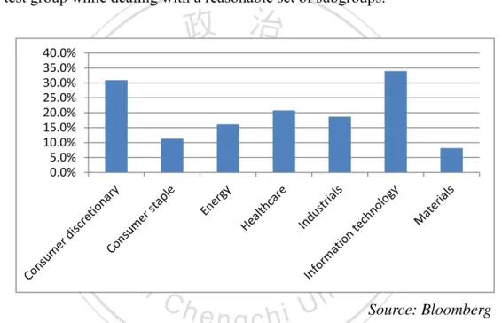
(22) . industry relative to other industries. Then, there is a trade-off between the quality of the study by comparing companies to a closer range of peers, and dealing with the complexity of determining multiple subgroups. Owing to that, companies will be grouped by industries according to the GICS Sector Group classification. The GICS Sector group classifies companies into 10 different segments. Removing financial companies, 9 groups are remaining. This classification will allow us to have a more accurate comparison between the control group and the test group while dealing with a reasonable set of subgroups.. 立. ‧. ‧ 國. 學. 40.0% 35.0% 30.0% 25.0% 20.0% 15.0% 10.0% 5.0% 0.0%. 政治大. n. er. io. sit. y. Nat. al. Ch. engchi. i n U. v. Source: Bloomberg. Figure 1: Distribution of Marginal-Debt Companies as a Percentage of Levered and Unlevered Companies Interestingly, we find no marginal-debt companies in both telecommunication and utilities sectors. Similarly, marginal-debt companies represent less than 10% of the materials sector universe. These three sectors are well known for being extremely capital intensive. This figure tells us that the marginal-debt capital structure strategy might not be compatible with some industries where high capital requirements are essential to be successful.. 15.

(23) . Both the sample of the information technology sector and the consumer discretionary sector represents about 30% of the marginal-debt companies each. They account for 31% and 34%, respectively, of their sector within the full data universe. These industries are well known for being less capital intensive. Moreover, the intangibility of assets in this sector might provide another reason why there is a high proportion of marginal-debt companies.. 3.3.. The Parameters. 政治大. In the scope of the study, we want to check whether any component of the trade-off formula. 立. could explain why some companies do not have debt on their balance sheets. Two main. ‧ 國. 學. elements influence the amount of debt a company should have to optimize its capital structure. The tax shield positively affect the amount of debt. It is defined by the corporate tax rate. ‧. multiplied by the amount of debt. The higher the tax rate is, the more debt a company should. Nat. sit. y. have. The second element is the bankruptcy cost, which is equal to the likelihood of default,. n. al. er. io. multiplied by the loss given default. There are no commonly agreed formula to calculate the. i n U. v. exact value for these parameters. However, we know other easily measurable parameters which. Ch. engchi. consistently affect them. In order to determine whether marginal-debt companies have higher likelihood of default than their indebted peers, we look at the Altman Z-score, a deleveraged version of the Altman Z-score, and the volatility of operational cash flows. Regarding the loss given default, we analyze the asset tangibility, the available collateral to total equity and financial debt, and the operational cash flow to total equity and financial debt. We assume all those criteria to be equally important in explaining the absence of debt in our test sample. A key issue when comparing marginal-debt companies with indebted companies is the capital structure. It might be obvious that companies which do not have debt have a lower chance and 16.

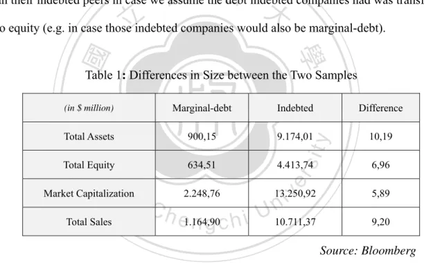
(24) . lower cost of bankruptcy that indebted one. Then, for each ratio we analyze, we try to select and adjust them so that the capital structure has a limited impact in the comparison. The idea is to virtually deleverage ratios from indebted companies to make them comparable to marginal-debt companies. Once indebted companies are virtually deleveraged, the comparison with marginal-debt companies ratios will tell us if there is any difference between the two samples in a situation where they both have no financial debt in their book. The approach can be explained by the following question: Would marginal-debt companies have higher cost of bankruptcy. 政治大. than their indebted peers in case we assume the debt indebted companies had was transformed. 立. into equity (e.g. in case those indebted companies would also be marginal-debt).. ‧ 國. 學. Table 1: Differences in Size between the Two Samples Difference. Total Assets. 900,15. 9.174,01. y. 10,19. Total Equity. 634,51. 4.413,74. 6,96. Nat. io. n. al. Market Capitalization Total Sales. Ch. 2.248,76. e1.164,90 ngchi. er. Indebted. sit. ‧. Marginal-debt. (in $ million). 13.250,92. v. 5,89. 10.711,37. 9,20. i n U. Source: Bloomberg Finally, as shown in the above table, both samples show significant size differences. Then for each financial figure studied, it is essential to find the proper denominator to have comparable ratios. Depending on the case, either sales, total assets, total equity, or market capitalization will be used as size denominator. Our choice for each specific case is explained later.. 17.

(25) . 3.3.1. The Tax Rate In the trade-off theory, the tax shield is the reason why company should take advantage of debt. By increasing their debts, companies can increase their tax shield. The tax shield is equal to the corporate tax rate multiplied by the amount of debt. Because the tax shield effect is directly related to the corporate tax rate, a first hypothesis is that marginal-debt companies might have a corporate tax rate close to zero. It would explain the absence of debt as a corporate tax rate close. 政治大 to have a much lower corporate tax rate than their indebted peers. In order to estimate a 立 to zero would not provide any tax shield. Obviously, we also expect marginal-debt companies. ‧ 國. 學. company´s corporate tax rate, we use the Bloomberg data RR037 (EFF_TAX_RATE). It is defined as the income tax expenses divided by the pretax income.. ‧. 3.3.2. The Bankruptcy Cost. sit. y. Nat. io. er. The bankruptcy cost is the second and last element of the equation to be analyzed. It is defined as the probability of default multiplied by the loss observed in case of default. A high. al. n. v i n bankruptcy cost could be a good C explanation h e n gofcthehexistence i U of marginal-debt companies. The. first component of this parameter, is already filtered with the Altman Z-score. All companies analyzed in the study should have, according to the Altman Z-score, a low probability of default. However, it might still be interesting to analyze the difference in score between marginal-debt and indebted companies. A second approach is to look at the cash flow volatility. To measure it, we look at the operational cash flow volatility. A higher cash flow volatility increases the probability of default of a company because of the uncertainty of its cash generation. While calculating and comparing the average corporate tax between our two samples was intuitive and provides a clear numerical value which could be used to estimate the tax shield 18.

(26) . effect, estimating the cost of bankruptcy is more difficult and less precise. Because this thesis does not aim to calculate an exact value for the cost of bankruptcy, but to determine whether marginal-debt companies have a higher bankruptcy cost than their indebted peers. Then, the study will focus on comparing key parameter affecting the cost of bankruptcy rather than estimating a value for cost of bankruptcy. Probability of default. 政治大. The probability of default is defined as the percent chance that a company goes bankrupt during. 立. a defined time horizon. Most common way to determine the probability of default of a company. ‧ 國. 學. is to look at its credit rating. However, this data is not available for all the data sample. Hence, as mentioned earlier, we use the Altman Z-score as a substitute for credit rating. Companies. ‧. have already been filtered on their Altman Z-score. They all have a score above 3 for three. Nat. sit. y. consecutive years between 2011 and 2013, meaning that they all have the healthy financials. n. al. er. io. which should easily allow them to access debt. In order to go further and check if there is any. i n U. v. difference in terms of likelihood of default between indebted companies and marginal-debt. Ch. engchi. companies, we first compare their Altman Z-score.. As a reminder, the Altman Z-score is calculated with the following formula: 1.2. 1.4. 3.3. 0.6. Where. X . 0.6 ∗ Market Capitalization Total Liabilities. 19.

(27) . In this formula, X4 is equal to the market capitalization divided by the total liabilities. This factor of the equation is the only one which is significantly impacted by the capital structure of the company. Then, to reduce the impact of capital structure in the analysis, we deleverage the Z-score formula by modifying the X4 component as shown in the following formula:. 0.6 ∗ Total Liabilities – . Deleveraged X . /. ∗ Market Capitalization &. 政治大 In order to find the above formula, we virtually turn Short & Long Term Financial Debt into 立. ‧ 國. 學. equity. Owing to that, we removed it from the total liabilities in the denominator. Moreover, we took the assumption that transforming Short & Long Term Financial Debt into equity would. ‧. also increase its market capitalization by the percentage increase of equity resulting from this. sit. y. Nat. operation.. n. al. er. io. In a third approach, we study the volatility of operational cash flow for each company. We. i n U. v. select operational cash flow instead of cash flow as it only focuses of companies operations and. Ch. engchi. allows us to ignore capital structure factors (e.g. debt reimbursement). A higher volatility of cash flow means that the cash generated by a company is not stable, it is more likely that during some years it has an extremely low cash flow generation. It is problematic when this low cash flow generation during some time does not allow the company to reimburse its debt or even finance its own operations. Then, a company with higher cash flow volatility will have a higher likelihood of default. We calculate the volatility of operational cash flow generated by each company during the 3 years period and then divide it by the average operational cash flow generated by the same company over the same period, as described by the formula bellow:. 20.

(28) . %. Where. ̅. is the standard deviation of operational cash flow ̅ %. is the average operational cash flow is the operational cash flow volatility. Dividing the operational cash flow by the average cash flow allows us to express the volatility in terms of percentage, so that we can compare companies regardless of their size.. 立. Loss given default. 政治大. ‧ 國. 學. The loss given default represents the money the lender would lose in case of default of the. ‧. borrowing company. A company with a high amount of tangible assets will have more collateral to sell in case of default, meaning that it reduces its loss given default. Then, we could expect. y. Nat. n. al. er. io. sit. marginal-debt companies to have a lower amount of tangible assets.. i n U. v. When a financial institution lends money to a company it often requires the company to use its. Ch. engchi. assets as collateral to secure the loan. In this case, if the company goes into bankruptcy, the bank can recover a part of the money it let by selling the assets. The amount a company´s worth in case of bankruptcy, called the liquidation value, is mainly represented by the amount of physical assets it owns. Physical assets are real estate, fixtures, equipments and inventories. Bloomberg provides the information for physical assets, called tangible assets. A higher tangible assets values implies a lower bankruptcy cost. We then study the asset tangibility of marginal-debt companies and compare it with their indebted peers. We expect marginal-debt companies to have a lower asset tangibility ratio, meaning that they have a higher proportion of intangible assets, which are much less valuable as collateral. The asset tangibility ratio is 21.

(29) . calculated by dividing tangible assets into total assets. The cash flow represents the amount of cash a company is generating. When applying for debt, it is a key parameter as it indicates the company’s ability to reimburse its debt. Insufficient cash flow compared to the amount of debt a company has. In practice, most banks allow their customers to have debt equals to three times of the free cash flow. The loss given default is defined as the expected loss a borrower will face in case the company. 政治大. he lend money to, goes bankrupt. Tangibility of asset is the first key variable for estimating the. 立. loss given default as tangible assets have a clear value given by the market, while intangible. ‧ 國. 學. assets are more difficult to value and sell. For instance, the value of the real estate a company owns is given by the real estate prices. In case of bankruptcy, we know that these assets can. ‧. easily be sold at a price close to market prices. On the other hand, patents or brand value do not. Nat. sit. er. io. scenario.. y. have clearly defined market value and are much more difficult to sell, especially in a stress. al. n. v i n C h the average netUamount of tangible assets each sample In a second approach, we try to quantify engchi has. This number is calculated by subtracting short and long term financial debt to the amount. of tangible assets the company has. This variable tells how much tangible assets companies have left when selling part of them to reimburse the amount of financial debt they have. The resulting number provides a good indicator of the quantity of collateral which could be used for new debt issuance. Because both our sample have significant size difference, we use total equity as a denominator. It will help us having a sound comparison between the two samples. Moreover, it will help us interpreting the ratio by telling us, as a percentage of equity, how much asset can potentially be used as collateral for new debt issuance. The formula applied here is as 22.

(30) . following:. Tangible Assets Short &. Short &. Beside assets which can be used as collateral to secure the loan in case of bankruptcy, cash flow generated by a company´s operations are the main source of cash used to reimburse debt. The. 政治大 default is. To properly compare the two samples´ cash flow, we divide the operating cash flow 立 higher the cash flow is relative to the amount of debt the company has, the lower the loss given. ‧ 國. ‧. 學. of a company by its total equity and total financial debt as describe in the following formula:. Operational Cash Flow Short &. er. io. sit. y. Nat Statistical Method. al. n. 3.4.. Ch. engchi. i n U. v. For each financial parameter, we extract the data for fiscal year 2011, 2012, and 2013 (FY2011, FY2012, and FY2013). We then calculate the average for the period. When having both samples mean and standard deviation, we test their mean having the following hypothesis: :. ". ". :. ". ". In order to test this hypothesis, we compute a two sided Welch t test. The Welch t test is an adaptation of the classical Student t test when samples are expected to have different standard deviations. The t statistic from the Welch t test is calculated with the following formula: 23.

(31) . ̅ ̅. ⁄ Where. ⁄. ̅ , and ̅ are the sample means , and. are the sample variances. , and. are the sample sizes. We need the degree of freedom to compute the test. The degree of freedom is calculated with the formula bellow:. 立. ‧ 國. . .. ⁄. ⁄ 1. 1. ‧. ̅ , and ̅ are the sample means. y. sit. are the sample variances. er. are the sample sizes. io. , and. Nat. , and. 學. Where. 政治大. al. n. v i n Cwe For all tests conducted in the study, an extremely large value for the degree of freedom. h ehave ngchi U. Hence, we will consider it to be close to infinite. We test all sample means at 90%, 95% and. 99% significance level. Then, H0 will be rejected at all respective significance level in case we find the t statistic superior to 1.645, 1.960, and 2.576. This statistical method has been used in previous literature such as Agrawal and Nagarajan (1990), Strebulav and Yang (2013), and Devos et. Al. (2012).. 24.

(32) . 4. Data and Analysis 4.1.. Defining the sample. The study aims at analyzing US public companies having more than 100 million US dollars in revenues in 2011. This first criterion will allow us to avoid companies which could not access to debt because of their size. Also, big companies might be more aware of capital structure challenges and act according to it. Most of the time, smaller companies do not have a financial. 政治大. department and might not think of their financial strategy carefully.. 立. Because they have an extremely specific structure which might not be analyzed the same way. ‧ 國. 學. as other industries, financial companies will be removed from the study. Most financial ratios. ‧. used in the study are not relevant for financial companies of require some adjustments. Moreover, financial companies are well known for having opaque financials with complex. y. Nat. n. al. er. io. from the study.. sit. network of subsidiaries. Those are the main reasons why financial companies are dismissed. Ch. engchi. i n U. v. Companies will have to show at least 2 years of financial history prior to the test period. Age is actually another key issue when seeking debt financing. We believe that companies with more than 2 years of financial history will have enough to show to financial institutions to easily subscribe debt. After setting those first parameters on Bloomberg, we find 1907 US non financial public companies having more than $100 million revenue in 2011 and at least 2 years of financial history before 2011. Out of those 1907 companies, 313 (16.4%) are marginal-debt companies and 1594 (83.6%) are indebted companies.. 25.

(33) . As mentioned earlier, Devos et al. (2012) find the evidence than most companies do not have debt in their balance sheet due to their inability to raise debt either from banks or financial institutions. It actually sounds normal that companies facing a high bankruptcy risk would have difficulties to convince banks or financial markets to lend them additional money. Then, most marginal-debt companies may be in this situation and have no other choice than not having debt. This phenomenon is logical and well documented in the literature. Indeed, as this study aims at studying marginal-debt companies which use this strategy as a choice, we want to remove. 政治大. companies with high bankruptcy risk from the study. While in real life, each company is a. 立. specific case which involves many different parameters to be taken into account in order to. ‧ 國. 學. assess its capacity to raise debt, this study will use a single variable, the Altman Z-score. Using a single and universal variable avoids any bias in the study. It also helps us avoiding too much. ‧. complexity and restrictions in the data selection. Altman Z-score was introduced by Edward I.. Nat. sit. y. Altman in 1968 in order to predict company bankruptcy. It is widely used in academic studies. n. al. er. io. for analyzing bankruptcy risk and its impact on other financial indicators. In the scope of this. i n U. v. study, we will use the Altman Z-score given under the VM001 (ALTMAN_Z_SCORE). Ch. engchi. mnemonic in Bloomberg and calculated with the following formula : Z Where. 1.2X. 1.4X. 3.3X. 0.6X. 1X. X1 = (Total Current Assets – Total Current Liabilities) / Total assets X2 = Retained Earnings / Total Assets X3 = (Pretax Income + Interest Expense) / Total Assets X4 = Market Capitalization / Total Liabilities X5 = Revenue / Total Assets. 26.

(34) . Using the above formula, a Z-score below 1.81 indicates a high bankruptcy risk while a score above 3 indicates a company in a healthy situation. In this study, companies will be selected if they show a Z-score above 3 from 2011 to 2013. In Altman (2000), using a cutoff score of 2.675 the Altman Z-score proved to be between 82% and 94% accurate predicting bankruptcy one year in advance. Type II errors (declaring that a firm would bankrupt while it actually does not) is between 15% and 20%. Those results are reasonable with the purpose of the study and help eliminated a major proportion of companies which are not able to raise debt. Type II errors will. 政治大. only penalize the study by reducing the sample. This is not a key issue as it should not affect the. 立. results of the study. On the other hand, type I error would penalize the study as it would include. ‧ 國. 學. companies with high bankruptcy risk in the study. This is why, as long as the test sample is not too small, it is better for this study to select a conservative Z-score as a selection parameter. Our. ‧. sample will include companies which have a Z-score above 3 for each consecutive year. Nat. er. io. sit. y. between 2011 and 2013.. In addition to the Altman Z-score, we require companies to have positive net income for each. al. n. v i n consecutive year between 2011Cand With thisUsecond parameter indicating that all h e2013. ngchi companies in our sample should be profitable, there is a much higher probability that all marginal-debt companies in the sample could easily access debt. Using those two financial health criteria, 718 companies are remaining. It represents 37.7% of the total number of US non financial public companies having more than $100 million revenue. in 2011 and at least 2 years of financial history before 2011. The marginal-debt sample contains 167 (23.2%) companies against 551 (76.6%) for the indebted sample. We can notice that indebted companies were much more affected by the financial health criteria that marginal-debt companies. It tells us that, in average, marginal-debt companies are less risky than their 27.

(35) . indebted peers. Among those marginal-debt companies, 100 (60%) companies have strictly no debt from 2011 to 2013, and 74 (44%) have strictly no debt from 2009 to 2013. On the other hand, 43 companies had a debt-to-equity ratio above 5% in 2009, 2010, or both 2009 and 2010. 13 of them have a debt ratio above 20% in 2009, 2010, or both 2009 and 2010. The average debt-to-equity ratio for the period (e.g. from 2011 to 2013) is 0,36%.. 政治大. On the other hand, we have 551 indebted companies having a 56,29% average debt-to-equity. 立. ratio. Sixty three of those indebted companies had a debt-to-equity ratio below 5% in both 2010. ‧ 國. 學. Indebted companies. Marginal-debt companies. sit. y. ‧. TEST GROUP. Nat. CONTROL GROUP. US non financial public companies. io. al. er. and 2009.. v. n. Available information for at least 2 years before the study period. Ch. engchi. i n U. Total revenues > $100M in 2011 Altman Z-score > 3 from 2011 to 2013 Net income > 0 from 2011 to 2013 D/E > 0.05 for at least one year D/E < 0.05 from 2011 to 2013 between 2011 and 2013 Figure 2: Sampling Summary. 28.

(36) . 4.2.. Analysis of the Sample Data. 4.2.1. Tax Rate In order to determine whether marginal-debt companies could benefit from the tax shield, we extracted the effective tax rate of all companies from 2011 to 2013. We find an average effective tax rate of 31.44% for marginal-debt companies, with a 11.32% standard deviation. The average effective tax rate is significantly different from zero at a 99% confidence level. Then,. 政治大 their balance sheet. The tax component of the trade-off theory formula fails at explaining the 立. there is no evidence that marginal-debt should not benefit from the tax shield if they had debt in. ‧ 國. 學. behavior of marginal-debt companies.. More interestingly, we also studied the effective tax rate of indebted companies from 2011 to. ‧. 2013. For those companies, we find an average effective tax rate of 29.78% with a 11.27%. Nat. sit. y. standard deviation. Comparing the two samples average effective tax rate, we find a t-statistic. n. al. er. io. equal to 1.66. At a 95% confidence level, average effective tax rate of indebted companies and. i n U. v. marginal-debt companies do not have any significant difference, while the average effective tax. Ch. engchi. rate of the marginal-debt sample is significantly higher at a 90% significance level. It means that marginal-debt companies could at least have the exact same benefit as indebted companies from the tax shield.. 29.

(37) . Table 2: Corporate Tax Rate Marginal-debt. Indebted mean. Difference. t-statistic. 33%. 31%. 2%. 0,803. Consumer staple. 35%. 32%. 3%. 1,996. Energy. 35%. 30%. 5%. 2,098. Healthcare. 30%. 29%. 1%. 0,445. Industrials. 34%. 31%. 3%. 1,913. Information technology. 28%. 3%. 1,278. Materials. 25%. -6%. -0,783. 2%. 1,661. mean Consumer discretionary. 立31%. Global. 26% 政治 31% 大 30%. ‧ 國. 學 ‧. 4.2.2. Cost of Bankruptcy. Source: Bloomberg. sit. y. Nat. As explained earlier in the sample selection process, only US public companies having more. n. al. er. io. than $100 million in revenues, two years of financial history before the study period, an Altman. v. Z-score above 3 between 2011 and 2013, and positive net income for the full study period are. Ch. engchi. i n U. selected. We believe those criteria are sufficient to support the hypothesis that those companies could easily have access to debt. Because financial health and debt eligibility are key factor for our study, some other financial ratios will be studied to validate our hypothesis. The Altman Z-score provides a good indicator of the likelihood of default of the company. The net income filter ensures that all companies are profitable. In addition to those parameters, we want to have a deeper analysis of the asset structure and the cash flow.. 30.

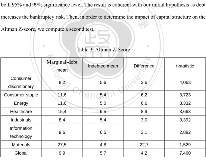
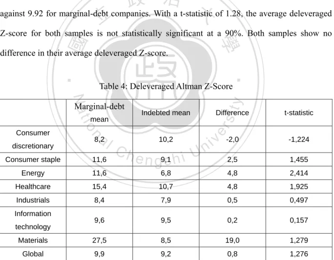
(38) . Likelihood of default We compute the average Altman Z-score for both samples. Marginal-debt companies show a significantly higher Z-score in all GICS sector, ranging from 1.46 times higher in the consumer discretionary sector, to 5.72 times higher in the materials sector. Globally, the average Z-score for marginal-debt companies over the 3 years period is 9.92 against 5.74 for indebted companies. With a t-statistic of 7.46, we can say that the average Z-score of marginal-debt. 政治大 both 95% and 99% significance level. The result is coherent with our initial hypothesis as debt 立. companies is significantly higher than the average Z-score of indebted companies. This holds at. ‧ 國. 學. increases the bankruptcy risk. Then, in order to determine the impact of capital structure on the Altman Z-score, we compute a second test.. al. n. discretionary. 8,2. Ch. y. sit. io. mean. Indebted mean. 5,6. e n g5,4c h i. Difference. er. Nat. Marginal-debt. Consumer. ‧. Table 3: Altman Z-Score. i n U. v. t-statistic. 2,6. 4,063. 6,2. 3,723. Consumer staple. 11,6. Energy. 11,6. 5,0. 6,6. 3,332. Healthcare. 15,4. 6,5. 8,9. 3,663. Industrials. 8,4. 5,4. 3,0. 3,392. 9,6. 6,5. 3,1. 2,882. Materials. 27,5. 4,8. 22,7. 1,529. Global. 9,9. 5,7. 4,2. 7,460. Information technology. Source: Bloomberg. 31.

(39) . As mentioned in the previous section, X4 is equal to the market capitalization divided by the total liabilities. It is the main component affected by the capital structure in the Altman Z-score formula. We isolate this component and compare its average value for both the marginal-debt and the indebted sample. As a result, marginal-debt companies show a 6.72 average value for X4 against 2.26 for indebted companies. This leads to a 4.46 difference between both samples, while marginal-debt companies had a 4.18 higher Z-score.. 政治大 against 9.92 for marginal-debt companies. With a t-statistic of 1.28, the average deleveraged 立. Using the deleveraged X4, we find a 9.16 average deleveraged Z-score for indebted companies. ‧ 國. 學. Z-score for both samples is not statistically significant at a 90%. Both samples show no difference in their average deleveraged Z-score.. ‧. discretionary. al. n. Consumer. 8,2. Ch. sit. io. mean. Indebted mean. 10,2. e n g9,1c h i. Difference. er. Nat. Marginal-debt. y. Table 4: Deleveraged Altman Z-Score. i n U. v. t-statistic. -2,0. -1,224. 2,5. 1,455. Consumer staple. 11,6. Energy. 11,6. 6,8. 4,8. 2,414. Healthcare. 15,4. 10,7. 4,8. 1,925. Industrials. 8,4. 7,9. 0,5. 0,497. 9,6. 9,5. 0,2. 0,157. Materials. 27,5. 8,5. 19,0. 1,279. Global. 9,9. 9,2. 0,8. 1,276. Information technology. Source: Bloomberg. 32.

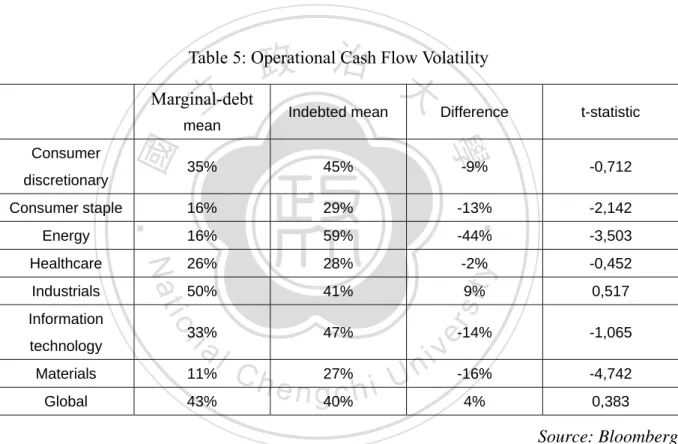
(40) . The indebted company sample shows a 39.5% average operational cash flow volatility while the marginal-debt sample shows a 42.2% average operational cash flow volatility. With a t-statistic of 0.30, we find no statistical difference between the two global samples in terms of average operational cash flow volatility at both 95% and 90% significance level. The materials sector, the energy sector and the consumer staple samples are the only one showing a significantly higher volatility for the marginal-debt sample.. 政治大 Marginal-debt 立 Indebted mean Difference mean. Energy. 16%. 59%. -44%. -3,503. 26%. 28%. -2%. -0,452. 50%. 41%. 0,517. 33%. al. 47%. n. technology. -2,142. io. Information. -13%. Nat. Industrials. 29%. Materials. 11%. Global. 43%. Ch. y. 16%. Healthcare. -0,712. sit. Consumer staple. t-statistic. -9%. 9%. er. 45%. ‧. 35%. discretionary. 學. Consumer. ‧ 國. Table 5: Operational Cash Flow Volatility. n U e n g40% chi 27%. iv. -14%. -1,065. -16%. -4,742. 4%. 0,383. Source: Bloomberg. 33.

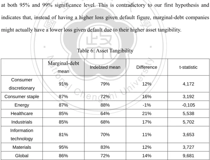
(41) . Loss given default As mentioned in the previous section, we expect marginal-debt companies to have a lower asset tangibility ratio, asset tangibility being defined as tangible assets divided by total assets. However, the data shows us that for all GICS sector, marginal-debt companies have an average assets tangibility ratio at least as high as their indebted peers. Globally, with a 0.86 asset tangibility ratio, marginal-debt companies´ assets are 19% more tangible than those indebted. 政治大 at both 95% and 99% significance level. This is contradictory to our first hypothesis and 立 companies. The superior asset tangibility of the marginal-debt sample is statistically significant. ‧ 國. 學. indicates that, instead of having a higher loss given default figure, marginal-debt companies might actually have a lower loss given default due to their higher asset tangibility.. al. n. discretionary. 91%. Ch. y. sit. io. mean. Indebted mean. 79%. e n g72% chi. Difference. er. Nat. Marginal-debt. Consumer. ‧. Table 6: Asset Tangibility. i n U. v. t-statistic. 12%. 4,172. 16%. 3,192. Consumer staple. 87%. Energy. 87%. 88%. -1%. -0,105. Healthcare. 85%. 64%. 21%. 5,538. Industrials. 85%. 68%. 17%. 5,702. 81%. 70%. 11%. 3,653. Materials. 95%. 83%. 12%. 3,727. Global. 86%. 72%. 14%. 9,681. Information technology. Source: Bloomberg. 34.

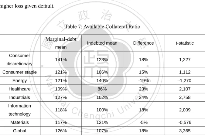
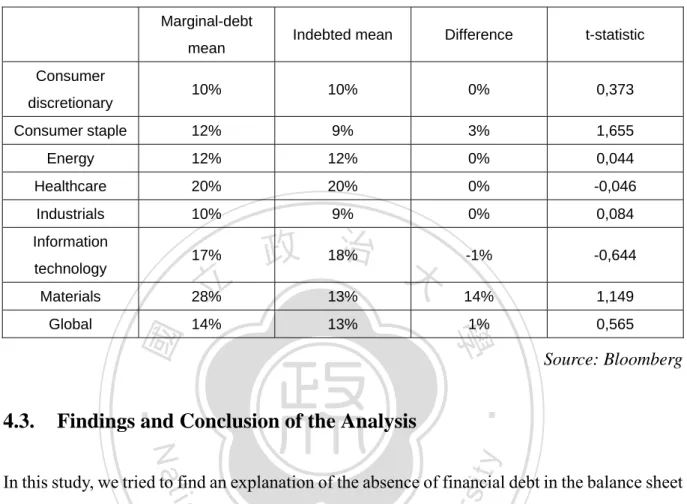
(42) . When analyzing the available collateral ratio, a higher ratio indicates that a company has more collateral available for new debt issuance. Results are again in favor of marginal-debt companies. Marginal-debt companies have on average 1.26 times their total equity in tangible assets net of financial debt, against 1.07 for indebted companies. With a t-stat of 3.37, we can say that marginal-debt companies have significantly higher ratio at both 95% and 99% significance level. It reinforces the fact that marginal-debt companies might not suffer from higher loss given default.. 政治大立Table 7: Available Collateral Ratio. technology. 18%. 1,227. 121%. 106%. 15%. 1,112. 121%. 140%. -19%. -1,270. 109%. 86%. 23%. 2,107. 127%. al. 102%. n. Information. 123%. io. Industrials. 141%. 118%. Materials. 117%. Global. 126%. Ch. y. sit. Healthcare. t-statistic. Nat. Energy. Difference. er. Consumer staple. Indebted mean. mean. ‧. discretionary. ‧ 國. Consumer. 學. Marginal-debt. 24%. 2,758. 18%. 2,009. 121%. -5%. -0,576. 107%. 18%. 3,365. n U engchi 100%. iv. Source: Bloomberg Finally, by looking at the operational cash flow ratio, we find that the marginal-debt sample average ratio is 21.66% against 17.02% for the indebted sample. With a t-statistic of 3.43, the marginal-debt sample generates significantly higher operational cash flows compared to its total equity plus financial debt at both 95% and 99%.. 35.

(43) . Table 8: Operational Cash Flow Ratio Marginal-debt. Indebted mean. Difference. t-statistic. 10%. 10%. 0%. 0,373. Consumer staple. 12%. 9%. 3%. 1,655. Energy. 12%. 12%. 0%. 0,044. Healthcare. 20%. 20%. 0%. -0,046. Industrials. 10%. 9%. 0%. 0,084. -1%. -0,644. mean Consumer discretionary. Information. 17%. technology. 28%. 13%. 14%. 1,149. Global. 14%. 13%. 1%. 0,565. Findings and Conclusion of the Analysis. Source: Bloomberg. Nat. sit. y. ‧. ‧ 國. Materials. 學. 4.3.. 立. 治政 18% 大. io. er. In this study, we tried to find an explanation of the absence of financial debt in the balance sheet of marginal-debt companies by looking at their corporate tax rate, bankruptcy risk, and cost of. al. n. v i n C h marginal-debt companies bankruptcy. We find that on average, have similar, or even higher engchi U. corporate tax rate than their indebted peers. Increasing their debt level should give them the same tax shield as indebted companies. The corporate tax rate does not explain why marginal-debt companies do not use debt. Similarly, marginal-debt companies do not have higher bankruptcy risk, even when deleveraging the financials of indebted companies. Altman Z-score is significantly higher for marginal-debt companies. When removing the capital structure factor in the Altman Z-score, we find that marginal-debt companies have the same bankruptcy risk as indebted companies which we virtually deleveraged. The volatility of cash flow for both samples confirms the 36.

(44) . deleveraged Altman Z-score comparison, as we find no statistical difference between the two samples. Hence the likelihood of default also does not provide any explanation for the absence of debt in our test sample. Finally, we find that marginal-debt companies have significantly higher asset tangibility, higher available collateral, and higher operating cash flow ratio than indebted companies. More than not explaining why marginal-debt companies do not optimize their capital structure, this result. 政治大. tells us that marginal-debt might have higher increase in firm value by increasing debt than the control sample.. 立. ‧ 國. 學. None of the components of the trade-off theory explains why “marginal-debt” companies only have marginal-debt. Then the trade-off theory is not sufficient to explain this behavior. We do. ‧. not find any evidence that “marginal-debt” companies either have lower corporate tax, or. Nat. sit. y. higher bankruptcy cost, than their indebted peers. While we do not reject the trade-off theory,. n. al. er. io. we make the assumption that some other parameters outside the trade-off theory might explain. i n U. v. the marginal presence of debt for some companies. We suspect some behavioral factors to be. Ch. the reasons for this phenomenon.. engchi. 37.

(45) . 5. Suggestions on a Survey Questionnaire In this section, we enumerate possible behavioral reasons explaining the marginal-debt phenomenon and suggest a survey questionnaire to quantify the impact of those capital structure decisions. We believe that comparing the results of this survey between marginal-debt companies and indebted companies will help understand the marginal-debt phenomenon. The questionnaire covers three topics: the relationship between the manager and shareholders, the. 政治大. manager´s perceived benefit of leverage, and the manager´s perceived loss of flexibility and. 立. control due to financial debt. Along with those thee topics, we ask managers to provide four. ‧ 國. 學. numbers concerning the debt-to-equity ratios of their companies: the current debt-to-equity ratio of the company, the manager´s target debt-to-equity ratio, the maximum debt-to-equity. ‧. ratio the company could bear, and the maximum debt-to-equity ratio the manager could accept.. sit er. io. Relationship between the Manager and Shareholders. al. n. 5.1.. y. Nat. The full version of the suggested survey is in the appendix.. Ch. engchi. i n U. v. A key element to understand the marginal-debt phenomenon is to understand the difference between shareholders and managers incentives regarding debt structure. While the trade-off theory provides an optimal capital structure in the shareholders point of view, managers might have a different opinion. Morellec, Nikolov, and Schurhoff (2012) claim that the cost of debt to managers is three times higher than the cost of debt to shareholders, which would explain the low leverage puzzle. While managers have their own target capital structure which is expected to be lower than shareholders´ target, shareholders have tools to change managers´ incentives toward their own objectives. Novaes and Zingales (1995) argue that the risk of being replaced due to a takeover or to shareholders decision give managers the incentive to increase the 38.

(46) . leverage of the company. Debt is well known to be an efficient anti-takeover tool. In case of takeover, it is likely that the current manager of the company might be replaced. Similarly, if shareholders are unhappy with the manager´s decisions, they can decide to fire him and find a new manager. Considering this statement, we calculated the average seniority of CEO. Current CEO of marginal-debt companies have been employed for more than 11 years against 8 years for indebted companies. Morellec, Nikolov, and Schurhoff (2012) argue that a higher manager ownership and higher stock option payments also provide a good incentive for managers to. 政治大. better match shareholders´ target in terms of capital structure. However, it is interesting that we. 立. find our marginal-debt sample having a significantly higher insider ownership rate than the. ‧ 國. 學. indebted sample. On average, marginal-debt companies have 8.3% of insider ownership against 5.2% for indebted companies.. ‧. sit. y. Nat. For the reasons mentioned above, we expect the observed debt-to-equity ratio to differ from the. io. er. manager´s target debt to equity ratio depending on the relation between the manager and shareholders. That is why we decide to include some questions regarding this point in our. al. n. v i n C h managers and shareholders, survey. A better relationship between or a dominant position of engchi U managers, can help understanding the existence of marginal-debt companies. In case a manager. is debt averse, and has the confidence of shareholders, he can better follow his own capital structure strategy without facing the risk of being fired. We actually expect our marginal-debt sample to have good manager-shareholder relationship as marginal-debt managers have a larger ownership on average. Hence, our first category of question aims at understanding the nature and health of the relationship between both agents. Those questions are based on the above literature. Answers from those questions will provide an idea about the power the manager has regarding capital structure decisions. Those questions try to quantify the manager´s feeling. 39.

(47) . about how CEO friendly shareholders are, how secured his position is, how much pressure he receives from shareholders regarding capital structure decisions, and how his objectives and shareholders´ objectives differ in terms of capital structure strategy. We expect marginal-debt companies to have more CEO friendly shareholders. Managers from marginal-debt companies might receive less pressure from shareholders regarding capital structure decisions, and they might feel more confident about their position. Finally, we asks if the company is family owned Also, as mentioned in the literature, we expect the marginal-debt sample to have a higher. 政治大. proportion of family owned businesses.. 立 Benefits of Leverage. ‧ 國. 學. 5.2.. Even if theory is clear about the added value of financial leverage on firm value, the manager´s. ‧. perception might differ from theory. Hence, we ask their opinion about the following statements. Nat.  . sit er. Increasing debt could help diminishing the threat of takeover. al. v i n C h ratio can significantly I believe a superior debt-to-equity increase company value engchi U n. . io. . y. to valid or not this assumption:. Debt allows companies to enjoy tax shield. Overall, I consider financial debt as a useful tool for companies. In case managers of marginal-debt companies consider that financial debt is not a good tool for the company, if they have a low perceived value of the tax shield, and of the increase of company value from higher debt-to-equity ratio, or if they do not see debt as a means to decrease the threat of takeover, some efforts could be spent in convincing them that they might be wrong. It would help reaching a more optimal capital structure.. 40.

(48) . 5.3.. Value of Flexibility and Control. One reason mentioned by Morellec, Nikolov, and Schurhoff (2012) to explain the higher cost of debt for managers is that debt limits managerial flexibility. Managerial flexibility is defined as the management team´s ability to take its investment decisions depending on the business environment and opportunities offered to the management at any time. By having no debt, companies can easily access to debt at any time to capture new profitable opportunities.. 政治大 they already have too much debt. As mentioned in the article “Debt-free Zara looks beyond pain 立. Indebted companies might not be able to do so when facing capital intensive projects in case. ‧ 國. 學. in Spain”, marginal-debt companies can also better absorb economical shocks than their. indebted peers, as its cash flow is not penalized by any debt reimbursement. Also, banks often. ‧. ask for collateral, or restrictions on future investments and financial ratios before lending. sit. y. Nat. money to a company. Hence, this third category aims at assessing the perceived impact of debt. io. al. n. questions:. er. on flexibility and control of the company. This section gathers the following five statements and. Ch. engchi. i n U. v. . I consider debt to have a negative impact on the company´s flexibility.. . Debt holders might prevent me from making the optimal decisions for the company.. . In order to increase my debt level, I would accept to provide collateral.. . In order to increase my debt level, I would accept restrictions on my future investments.. . In order to increase my debt level, I would accept restrictions on some financial ratios.. . I believe my company has a high threat of takeover.. We expect marginal-debt company managers to claim that debt has a high negative impact on the company´s flexibility, and that debt holders might prevent them from making the optimal 41.