二維細胞類神經網路之一般模版: 全域花樣

國 立 交 通 大 學

應 用 數 學 所

碩 士 論 文

二維細胞類神經網路之一般模版：

全域花樣

Two-Dimensional CNN with General Template：

Global Patterns

研 究 生：許倖綺

指導教授：林松山 教授

二維細胞類神經網路之一般模版：

全域花樣

Two-Dimensional CNN with General Template ：

Global patterns

研 究 生：許倖綺 Student：Hsing-Chi Hsu

指導教授：林松山 Advisor：Song-Sun Lin

國 立 交 通 大 學

應 用 數 學 所

碩 士 論 文

Submitted to Department of Applied Mathematics College of Science

National Chiao Tung University in partial Fulfillment of the Requirements

for the Degree of Master

in

Applied Mathematics June 2007

二維細胞類神經網路之一般模版：

全域花樣

學生：許倖綺 指導教授：林松山 教授

國立交通大學應用數學學系﹙研究所﹚碩士班

摘

要

此篇論文是研究如何將 3×3 的花樣擴展為 4×4 的花樣，進而利用置換

矩陣去研究花樣生成的問題。從禁止集合的觀點來看，如果

c

是 3×3 中不

允許的花樣，則可以找到 4×4 中不允許的花樣是

F c

( )

≡

F c

( )

∪

F c

( )

(

)

(

)

F c

F c

∪

∪

，意指收集

c

分別落在 4×4 花樣中第一、二、三及第

四像限位置的所有 4×4 的花樣，我們也可找到其置換矩陣。因此，在二維

細胞類神經網路之一般模版中，我們知道每一區可允許的局部花樣，且利

用置換矩陣的遞迴公式，可找出全域的花樣。此外，可採用連結算子去估

計空間熵的下界。

Two-Dimensional CNN with General Template：

Global Patterns

student：Hsing-Chi Hsu Advisors：Dr.Song-Sun Lin

Department of Applied Mathematics

National Chiao Tung University

ABSTRACT

In this paper, we investigate how to extend 3×3 patterns to 4×4 patterns and

then we can use transition matrices created by Ban and Lin to study pattern gen-

eration problems. From the viewpoint of forbidden sets, if

c

is a forbidden

pattern in

∑

, then we can find the forbidden set in

∑

is

F c

( )

≡

F c

( )

∪

2

( )

( )

( )

F c

∪

F c

∪

F c

it means collecting all 4×4 patterns which

c

located

in the first, second, third, and the fourth quadrant of 4×4 patterns respectively,

then we also can find the transition matrix. Therefore, in two-dimensional CNN

with general template, we have knew the admissible local patterns, then we can

find global patterns by the recursive formula of transition matrix, Furthermore,

we can use connecting operators to estimate a lower bound of spatial entropy.

誌

謝

此篇論文的完成要感謝許多人的協助幫忙，讓它得以順利產生。首先，

要感謝我的指導教授 林松山教授，是您引領我進入研究的大門，教我要從

最自然的觀點去看事物，除了在學術研究上的教導之外，我得到更多的是

待人處世上應有的態度，您的人生智慧灌溉了我還未茁壯的心靈。僅此，

致上我最誠摯的敬意與謝意。

在研究所求學過程中，感謝榮超學長在知識與經驗上的傳授，讓我獲

益良多；感謝吟衡學姊總是很有耐心地為我解答困惑，並且在論文的撰寫

上提供寶貴的建議，我才能順利完成初稿；感謝志鴻學長、其儒學長、文

貴學長、忠澤學長及耀漢學長，我的研究所生活因你們而更加豐富；還有

我可愛的同學們：園芳、雅羚、碧維、千砡、慧萍和怡菁，因為你們的陪

伴與鼓勵，讓我不覺得孤單，更為我的生活添加了幾分精采。幸運如我，

能在研究所遇到這麼多優秀的師長、學長姐、同學和學弟妹們，和你們的

相遇，是我人生中最開心的事之一。

最後，我要感謝我親愛的家人們，因為你們無怨無悔的付出，讓我能

在一個安心的環境中平安長大；因為你們無私的愛，讓我能夠自在地做自

己想做的事，是你們成就了今天的我。在此，獻上我最感恩的心，感謝有

你們的陪伴與支持，往後，我會更努力朝我的目標邁進。

目

錄

中文摘要 ………

i

英文摘要 ………

ii

誌謝

………

iii

目錄

………

iv

1.

Introduction………

1

2.

Partition of the Parameters Space………

3

2.1

General template………

3

2.2

Square-cross template………

4

2.3

Diagonal-cross template………

5

2.4

Double-cross template………

6

3.

Ordering Matrices and Transition Matrices……

8

3.1

Ordering matrices for

………

8

3.1.1 General 3×3 patterns………

14

3.2

Transition matrices………

17

3.2.1 Transition matrices for

………

17

3.2.2 Transition matrices for general 3×3 patterns

19

4.

Connecting Operators and Computation of

Spatial Entropy………

20

4.1

Connecting operators………

20

4.2

Computation of spatial entropy………

22

1

Introduction

Many systems have been studied as models for spatial pattern formation in bi-ology,chemistry, engineering and physics.In Lattice Dynamical Systems(LDS), especially Cellular Neural Networks(CNNs) which has been proposed by Chua and Young, the set of global stationary solutions(global patterns) has received considerable attention in recent years.The CNNs without input terms are of the form

dxi,j dt = −xi,j+ X |k|≤1,|`|≤1 ak,lf (xi+k,j+`) + z, (i, j) ∈ Z2, (1.1) xi,j(0) = x0i,j (1.2)

Here the nonlinearity f is a piecewise-linear function of the form

f (x) = 1

2(|x+1|−|x−1|). (1.3)

The numbers ak,`, |k| ≤ 1, |`| ≤ 1, k, ` ∈ Z, are arranged in a 3 × 3 matrix form, which is

called a space-invariant A-template

A =      a−1,1 a0,1 a1,1 a−1,0 a0,0 a1,0 a−1,−1 a0,−1 a1,−1      (1.4)

The quantities xi,j denote the state of a cell Ci,j. If xi,j > 1(resp. xi,j < −1), then its

corresponding cell Ci,j is called a positively (resp. negatively) saturated cell and the state

is called + (resp. -) state. A situation in which |xi,j| = 1 (resp. |xi,j| < 1) is called a

transitional or marginal state (resp. or linear state). The output of a cell Ci,j defined as yi,j = f (xi,j), equals 1,-1 and xi,j when xi,j is a +,- and linear, respectively. The quantity z is called threshold or bias term which is related to an independent voltage source in an

electrical circuit.

Lattices play an important role in many scientific models, such as in modeling under-lying spatial structures. Notable examples include models arising from biology,chemical reaction and phase transitions,image processing and pattern recognition, and material science.

As generally known, stationary solutions ¯x = (¯xi,j) of (1.1) are essential for

under-standing CNN systems; their outputs ¯y = (f (¯xi,j)) are called patterns. Juang and Lin

[12]used ”building block” technique to study the patterns generation and obtained lower bounds of the spatial entropy for CNN with square-cross or diagonal-cross templates. For CNN with general templates, Hsu et al [11] investigated the generation of admissible local patterns and obtained the basic set for any parameter, i.e., the first step in studying the patterns generation problem. Later, Ban and Lin [14] constructed the ”ordering matrix” X2 for Σ2`×2` to study the patterns generation and obtained recursion formulas for Xn for

Σ2`×n` where ` > 1 is a fixed positive integer and n ≤ 2. The recursive formulas for Xn

imply the recursive formula for the associated transition matrices Hn(B) of Σ2`×n`(B).

Motivated by the transition matrices in [1], this work introduce how to find global pat-terns for each general template A and threshold z. First, we extension 3 × 3 admissible local patterns to 4 × 4 admissible local patterns, when given a basic set for any parame-ter.The method is considering the forbidden set, means that if ck is a forbidden pattern in

Σ3×3, we define F1(ck), F2(ck), F3(ck) and F4(cK) be sets collecting 4 × 4 patterns with ck

located at left-down, left-up, right-down and right-up respectively,then we can know that the forbidden patterns in Σ4×4 is F (ck) ≡ F1(ck) ∪ F2(ck) ∪ F3(ck) ∪ F4(ck). Therefore, if Bc_{is a forbidden set of local patterns in Σ}

3×3, then

[

ck∈Bc

F (ck) is the set with all forbidden

local patterns in Σ4×4. Then, we can find out the transition matrix is ◦(H2(ck)), ck∈ Bc,

and using the method of Ban and Lin, global patterns can be found, and spatial entropy is known: h(B) = lim

n→∞

logρ(Hn)

4n , the detail is in section 3.

The rest of this paper is organized as follows. Section 2 describes that the parameters space can be divided into finitely many subregions such that in each region (1.1) has the same mosaic patterns. Section 3 addresses the ordering matrix and transition matrix of patterns in Σ4×4, and the rule putting 3 × 3 patterns into 4 × 4 patterns such that

transition matrices can be found in Σ4×4. Section 4 presents the application of connecting

operators to estimate a lower bound of spatial entropy and take an example to compare with Juang and Lin’s ”building block” method.

2

Partition of the Parameters Space

In this section,according to [11],we partition the parameters space

P10_{= {(A, z) : A is a 3×3 real matrix and z ∈ R}1_{} (2.1)}

into finite subregions such that each region has the same mosaic pattern.

For a given mosaic solution ¯x, the state at cell Ci,j is +, i.e. ¯xi,j > 1, if and only if

(a−1)+z + X

|k|,|`|≤1,(k,`)6=(0,0)

ak,`y¯i+k,j+`> 0, (2.2)

where a = a0,0. Similarly, if the state at cell Ci,j is −, i.e. ¯xi,j < −1, if and only if

(a−1)−z − X

|k|,|`|≤1,(k,`)6=(0,0)

ak,`y¯i+k,j+`> 0. (2.3)

2.1 General template

For a given general template, like (1.4) denote

α = (a1,1, a1,0, a1,−1, a0,1, a0,−1, a−1,1, a−1,0, a−1,−1),

and

V = (yi+1,j+1, yi+1,j, yi+1,j−1, yi,j+1, yi,j−1, yi−1,j+1, yi−1,j, yi−1,j−1).

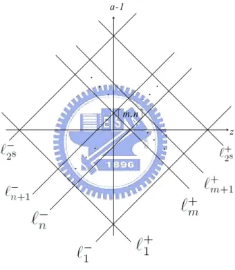
Vector α represents the surrounding template of A without center and vector V represents the surrounding outputs at cell Ci,j. Therefore, V is called a local pattern associated with

(A, z). we have two sets of parallel straight lines{`+

j }Nj=1 and {`−j }Nj=1 in (z, a − 1) plane, here L+ j (z, a) = (a − 1) + z + α · Vj, `+_j = {(z, a) : L+_j (z, a) = 0}, L− j(z, a) = (a − 1) − z − α · Vj, and `−_j = {(z, a) : L−_j (z, a) = 0},

for j = 1, · · · , N. In general,it may happen that α · Vi = α · Vi for some i 6= j, and in this

case `+

i = `+j and `−i = `−j .

If the values in template A are all different, there are 28 _{lines for both `}+

j and `−j, and

denote the region

[m, k] = {(z, a − 1) : L+

m(z, a) > 0 > L+m+1(z, a) and L−n(z, a) < 0 < L−n+1(z, a)}

which is bounded by`+

m, `+m+1 and `−n, `−n+1 as in Fig. 1. . . . . . . . . . .. a-1 z [m,n] .

Fig. 1. Partition of (z, a − 1) plane.

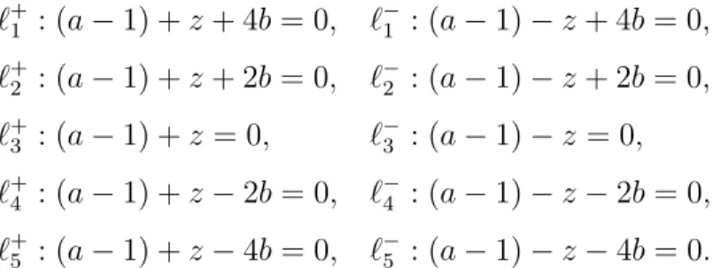
2.2 Square-cross template If template A is square-cross,e.g. A = A+≡      0 b 0 b a b 0 b 0     ,

the 5 + 5 lines are denoted by `+<sub>1</sub> : (a − 1) + z + 4b = 0, `−₁ : (a − 1) − z + 4b = 0, `+ 2 : (a − 1) + z + 2b = 0, `−2 : (a − 1) − z + 2b = 0, `+<sub>3</sub> : (a − 1) + z = 0, `−₃ : (a − 1) − z = 0, `+ 4 : (a − 1) + z − 2b = 0, `−4 : (a − 1) − z − 2b = 0, `+<sub>5</sub> : (a − 1) + z − 4b = 0, `−₅ : (a − 1) − z − 4b = 0.

Then the(z, a − 1) plane can be partition up to 36 subregions. For example, when b > 0, we have the bifurcation diagram as in Fig.2, details can be found in [12].

a 1

-Z

Fig. 2. Partition of (z, a − 1) plane with b > 0.

2.3 Diagonal-cross template If template A is diagonal-cross, e.g.,

A = A×_≡      c 0 c 0 a 0 c 0 c     

the 5 + 5 lines are denoted by `+ 1 : z + (a − 1) + 4c = 0, `−1 : z − (a − 1) + 4c = 0, `+<sub>2</sub> : z + (a − 1) + 2c = 0, `−₂ : z − (a − 1) + 2c = 0, `+ 2 : z + (a − 1) = 0, `−3 : z − (a − 1) = 0, `+<sub>4</sub> : z + (a − 1) − 2c = 0, `−₄ : z − (a − 1) − 2c = 0, `+ 5 : z + (a − 1) − 4c = 0, `−5 : z − (a − 1) − 4c = 0.

Then the(z, a − 1) plane can be partition up to 36 subregions like Fig.2. 2.4 Double-cross template

If template A is the form

A =      c b c b a b c b c     

we denote the 50 lines by

`+<sub>1</sub> : (a − 1) + z + 4b + 4c = 0 `−₁ : (a − 1) − z − 4b − 4c = 0 `+ 2 : (a − 1) + z + 4b + 2c = 0 `−2 : (a − 1) − z − 4b − 2c = 0 `+<sub>3</sub> : (a − 1) + z + 4b = 0 `−₃ : (a − 1) − z − 4b = 0 `+ 4 : (a − 1) + z + 4b − 2c = 0 `−4 : (a − 1) − z − 4b + 2c = 0 `+<sub>5</sub> : (a − 1) + z + 4b − 4c = 0 `−₅ : (a − 1) − z − 4b + 4c = 0 `+ 6 : (a − 1) + z + 2b + 4c = 0 `−6 : (a − 1) − z − 2b − 4c = 0 `+<sub>7</sub> : (a − 1) + z + 2b + 2c = 0 `−₇ : (a − 1) − z − 2b − 2c = 0 `+ 8 : (a − 1) + z + 2b = 0 `−8 : (a − 1) − z − 2b = 0 `+<sub>9</sub> : (a − 1) + z + 2b − 2c = 0 `−₉ : (a − 1) − z − 2b + 2c = 0 `+ 10 : (a − 1) + z + 2b − 4c = 0 `−10 : (a − 1) − z − 2b + 4c = 0 `+<sub>11</sub> : (a − 1) + z + 4c = 0 `−₁₁ : (a − 1) − z − 4c = 0 `+ 12 : (a − 1) + z + 2c = 0 `−12 : (a − 1) − z − 2c = 0 `+<sub>13</sub> : (a − 1) + z = 0 `−₁₃ : (a − 1) − z = 0

`+ 14: (a − 1) + z − 2c = 0 `−14: (a − 1) − z + 2c = 0 `+ 15: (a − 1) + z − 4c = 0 `−15: (a − 1) − z + 4c = 0 `+ 16: (a − 1) + z − 2b + 4c = 0 `−16: (a − 1) − z + 2b − 4c = 0 `+ 17: (a − 1) + z − 2b + 2c = 0 `−17: (a − 1) − z + 2b − 2c = 0 `+ 18: (a − 1) + z − 2b = 0 `−18: (a − 1) − z + 2b = 0 `+ 19: (a − 1) + z − 2b − 2c = 0 `−19: (a − 1) − z + 2b + 2c = 0 `+ 20: (a − 1) + z − 2b − 4c = 0 `−20: (a − 1) − z + 2b + 4c = 0 `+ 21: (a − 1) + z − 4b + 4c = 0 `−21: (a − 1) − z + 4b − 4c = 0 `+ 22: (a − 1) + z − 4b + 2c = 0 `−22: (a − 1) − z + 4b − 2c = 0 `+ 23: (a − 1) + z − 4b = 0 `−23: (a − 1) − z + 4b = 0 `+ 24: (a − 1) + z − 4b − 2c = 0 `−24: (a − 1) − z + 4b + 2c = 0 `+ 25: (a − 1) + z − 4b − 4c = 0 `−25: (a − 1) − z + 4b + 4c = 0

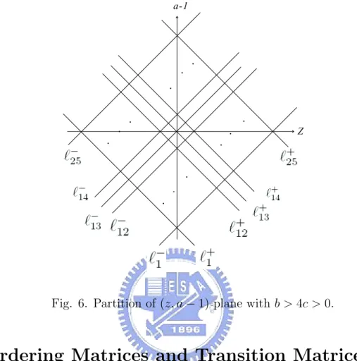
Then in each region of (b, c) plane as Fig. 5, the (z, a − 1) plane can be partitioned up to 26 × 26 subregions. For example, when b > 4c > 0, we have the bifurcation diagram as in Fig.6. b C 3 2 b= c 2 b= c 3 b= c 4 b= c b=c b= -c

. . . . . . . . . . . a-1 Z .

Fig. 6. Partition of (z, a − 1) plane with b > 4c > 0.

3

Ordering Matrices and Transition Matrices

This section describes two dimensional patterns generation, and the rule that 3 × 3 patterns putted into 4 × 4 patterns, then we can use pattern generation method to study the spatial entropy of CNN with general template,square-cross template or diagonal-cross template.

3.1 Ordering matrices for Σ4×4

For 2 × 2n pattern U = (uk), 1 ≤ k ≤ 2n in Σ2×2n,U is assigned the number

i = 1+

2n

X

k=1

As denoted by the 2 × 2n column pattern x2n;i, x2n;i= u2n−2 u2n u2n−3 u2n−1 ... ... u2 u4 u1 u3 (3.2)

In particular, when n = 2, as denoted byxi = x4;i,

i = 1 + 8 X k=1 28−k_u k (3.3) and xi = u6 u8 u5 u7 u2 u4 u1 u3 (3.4)

A 4 × 4 pattern can now be obtained by a horizontal direct sum of two 2 × 4 patterns, i.e,

xi1,i2 ≡ xi1 ⊕ xi2 ≡ u16 u18 u26 u28 u15 u17 u25 u27 u12 u14 u22 u24 u11 u13 u21 u23 (3.5) where ik = 1 + 8 X j=1 28−jukj , 1 ≤ k ≤ 2. (3.6)

Therefore, the complete set of all 216 _{patterns in Σ}

4×4can be listed by a 256 × 256 matrix

0 0 0 0 0 0 0 0 0 0 0 0 0 1 0 0 0 0 0 0 0 0 0 0 0 0 0 0 0 0 0 0 0 0 0 0 0 0 0 0 0 0 0 0 0 0 0 0 0 0 0 0 0 0 0 1 0 0 0 0 0 0 0 0 0 0 0 0 0 0 1 0 0 0 0 0 0 0 0 0 0 0 0 0 0 0 1 1 0 0 0 0 0 1 1 0 0 0 0 0 0 1 1 0 0 0 0 0 0 1 0 0 0 0 0 0 0 0 1 0 0 0 0 0 0 0 1 0 0 0 0 0 0 0 0 1 0 0 0 0 0 0 0 0 0 0 0 0 0 0 0 1 0 0 0 0 0 0 0 1 0 0 0 0 0 0 0 1 0 0 0 0 0 0 1 0 0 0 0 0 0 0 0 1 0 0 0 0 0 0 1 1 0 0 0 0 0 0 1 0 0 0 0 0 0 0 0 0 0 0 0 0 0 0 1 0 0 0 0 0 0 0 0 1 0 0 0 0 0 0 1 0 0 0 0 0 0 0 1 0 0 0 0 0 0 0 1 0 0 0 0 0 0 0 1 1 0 0 0 0 0 0 1 1 0 0 0 0 0 0 0 0 0 0 0 0 0 0 1 1 0 0 0 0 0 0 0 1 0 0 0 0 0 0 1 1 0 0 0 0 0 0 1 0 0 0 0 0 0 0 1 1 0 0 0 0 0 0 1 1 1 1 1 1 1 1 1 1 1 1 1 1 1 1 1 1 1 1 1 1 1 1 1 1 1 1 1 1 1 1 1 1 1 1 1 1 1 1 1 1 0 0 0 0 0 0 0 0 1 1 1 1 1 1 1 1 0 0 0 0 0 0 0 1 1 1 1 1 1 1 1 1 0 0 0 0 0 0 1 0 1 1 1 1 1 1 1 1 0 0 0 0 0 0 1 1 0 0 0 0 0 0 0 0 1 1 1 1 1 1 1 1 0 0 0 0 0 0 0 1 1 1 1 1 1 1 1 1 0 0 0 0 0 0 1 0 1 1 1 1 1 1 1 1 0 0 0 0 0 0 1 1 1 1 1 1 1 1 1 1

.

.

.

.

.

.

.

.

.

.

.

.

.

.

.

.

.

.

.

.

.

.

.

.

.

.

.

.

.

.

.

.

.

.

.

.

.

.

.

.

.

.

i.e, we are counting local patterns in Σ4×4by going through each row successively in Table

(3.7). Correspondingly, X2 can be referred to as an ordering matrix for Σ4×4. Similarly,

where yj l = u2l u4l u6l u8l u1l u3l u5l u7l (3.10) and jl = 1 + 8 X k=1 28−kukl, 1 ≤ l ≤ 2. (3.11)

A 4 × 4 matrix Y2 = [yj1,j2] can be obtained for Σ4×4. i.e, we have

0 0 0 0 0 0 0 0 0 0 0 0 0 0 0 0 0 0 0 0 0 0 0 0 0 0 0 0 0 0 0 0 0 0 0 0 0 1 0 0 0 0 0 0 0 1 0 0 0 0 0 0 0 0 0 0 0 0 0 0 0 0 0 1 0 0 0 0 0 0 0 0 0 0 0 0 0 0 1 0 0 0 0 0 0 0 0 0 0 0 0 0 0 0 1 1 0 0 0 0 0 0 0 0 0 0 0 0 0 1 0 0 0 0 0 0 0 0 0 0 0 0 0 0 0 1 0 1 0 0 0 0 0 0 0 0 0 0 0 0 0 1 1 1 0 0 0 0 0 0 0 0 0 0 0 0 0 1 0 1 0 0 0 0 1 0 0 0 0 0 0 0 1 1 0 0 0 0 0 0 1 0 0 0 0 0 0 0 1 1 0 0 0 0 0 0 0 0 0 0 0 0 0 0 1 0 0 0 0 0 0 0 0 0 0 0 0 0 0 0 0 0 0 0 0 0 0 0 0 0 0 0 0 0 0 0 1 0 0 1 0 0 0 0 0 0 0 0 0 0 0 0 1 0 1 0 0 0 0 0 0 0 0 0 0 0 0 0 1 0 1 1 0 0 0 0 0 0 0 0 0 0 0 0 1 1 0 0 0 0 0 0 0 0 0 0 0 0 0 0 1 1 0 1 0 0 0 0 0 0 0 0 0 0 0 0 1 1 1 0 0 0 0 0 0 0 0 0 0 0 0 0 1 1 1 1 1 1 1 1 1 1 1 1 1 1 1 1 1 1 1 1 1 1 1 1 0 0 0 0 0 0 1 1 1 1 0 0 1 1 1 1 0 0 0 0 0 0 1 1 1 1 0 1 1 1 1 1 0 0 0 0 0 0 1 1 1 1 1 0 1 1 1 1 0 0 0 0 0 0 1 1 1 1 1 1 1 1 1 1 1 1 1 1 1 1 1 1 1 1 1 1 0 0 0 0 1 1 1 1 1 1 0 0 0 0 1 1 0 0 0 0 1 1 1 1 1 1 0 0 0 1 1 1 0 0 0 0 1 1 1 1 1 1 0 0 1 0 1 1 0 0 0 0 1 1 1 1 1 1 0 0 1 1 1 1

.

.

.

.

.

.

.

.

.

.

.

.

.

.

.

.

.

.

.

.

.

.

.

.

.

.

.

.

.

.

.

.

.

.

.

.

.

.

.

that X2 can be represented by yj1,j2 as X2 =                        y1,1 · · · y1,16 · · · y16,1 · · · y16,16 y1,17 · · · y1,32 · · · y16,17 · · · y16,32 ... . .. ... · · · ... . .. ... y1,15·16+1 · · · y1,162 · · · y_16,15·16+1 · · · y_16,162 ... ... ... . .. ... ... ... y15·16+1,1 · · · y15·16+1,16 · · · y162_,1 · · · y₁₆2_,16 y15·16+1,17 · · · y15·16+1,32 · · · y162_,17 · · · y₁₆2_,32 ... . .. ... · · · ... . .. ... y15·16+1,15·16+1 · · · y15·16+1,162 · · · y₁₆2_,15·16+1 · · · y₁₆2_,162                        (3.13)

In (3.13), the indices j1, j2 are arranged by two Z-maps successively, as

1 15×16+1 15×16+2 2 16 . . . . . . . 17 18 32 2 . . . 16 . . . (3.14)

More precisely,X2 can be decomposed by

X2 =         Y2;1 y2;2 · · · Y2;16 Y2;17 Y2;18 · · · Y2;32 ... ... . .. ...         (3.15)

and Y2;k =         yk,1 yk,2 · · · yk,16 yk,17 yk,18 · · · yk,32 ... ... . .. ... yk,15·16+1 yk,15·16+2 · · · yk,162         16×16 . (3.16)

where X2 is arranged by a Z-map (Y2;k) in (3.15) and each Y2;k is also arranged by a

Z-map (ykl) in (3.16).Therefor, the indices of y in (3.13) consist of two Z-maps.

Now, we can state recursion formulas for higher ordering matrix Xn = [xn;i1i2]16n×16n

as follows.

Proposition 3.1 ([14])

For any n ≥ 2, Σ4×2n = {yj1j2···jn}, where yj1j2···jn ≡ yj1j2⊕yˆ j2j3⊕ · · · ˆˆ ⊕yjn−1jn, 1 ≤ jk ≤

162 _{and 1 ≤ k ≤ n. Furthermore, the ordering matrix X}

ncan be decomposed by n Z-maps

successively as Xn =         Yn;1 Yn;2 · · · Yn;16 Yn;17 Yn;18 · · · Yn;32 ... ... · · · ... Yn;15·16+1 Y15·16+2 · · · Yn;162         , Yn;j1···jk =         Yn;j1,··· ,jk,1 Yn;j1,··· ,jk,2 · · · Yn;j1,··· ,jk,16 Yn;j1,··· ,jk,17 Yn;j1,··· ,jk,18 · · · Yn;j1,···jk,32 ... ... . .. ... Yn;j1,··· ,jk,15·16+1 Yn;j1,···jk,15·16+2 · · · Yn;j1,···jk,162         , for1 ≤ k ≤ n − 2, and Yn;j1···jn−1 =         yj1,··· ,jn−1,1 yj1,··· ,jn−1,2 · · · yj1,··· ,jn−1,16 yj1,··· ,jn−1,17 yj1,··· ,jn−1,18 · · · yj1··· ,jn−1,32 ... ... . .. ... yi1,··· ,jn−1,15·16+1 yj1,··· ,yn−1,15·16+2 · · · yj1,··· ,jn−1,162         .

3.1.1 General 3 × 3 patterns

Definition 3.2 Σ3×3 is the set of all 3 × 3 patterns with two different symbols,i.e,

Σ3×3=          `−1,1 `0,1 `1,1 `−1,0 `0,0 `1,0 `−1,−1 `0,−1 `1,−1 : `i,j ∈ {0, 1}         

For ci ∈ Σ3×3, ci is assigned the number

i = 1 + `1,1+ 2`1,0+ 22`1,−1+ 23`0,1+ 24`0,0+ 25`0,−1+ 26`−1,1+ 27`−1,0+ 28`−1,−1.

Definition 3.3 Given ck∈ Σ3×3,

(i) ck is located in the first quadrant(right-up) of the 4 × 4 pattern in (3.5)

Let u25= `0,0, u14 = `−1,−1, u17 = `−1,0, u18 = `−1,1, u22 = `0,−1, u24 = `1,−1, u26 = `0,1, u27= `1,0, u28= `1,1. and let k1 = {1+`−1,1+2`−1,0+22u16+23u15+24`−1,−1+25u13+26u12+27u11 : u1j ∈ {0, 1}} and k2 = {1 + `1,1+ 2`1,0+ 22`0,1+ 23`0,0+ 24`1,−1+ 25u23+ 26`0,−1+ 27u21 : u2j ∈ {0, 1}} Then we define F1(ck) ≡ {xi1,i2 : i1 ∈ k1, i2 ∈ k2}

be the set of all patterns with index i1 satisfy k1 and i2 satisfy k2 in Σ4×4.

(ii) ck is located in the second quadrant(left-up) of the 4 × 4 pattern in (3.5)

u22 = `1,−1, u25 = `1,0, u26= `1,1. and let k1 = {1+`0,1+2`0,0+22`−1,1+23`−1,0+24`0,−1+25u13+26`−1,−1+27u11 : u1j ∈ {0, 1}} and k2 = {1 + u28+ 2u27+ 22`1,1+ 23`1,0+ 24u24+ 25u23+ 26`1,−1+ 27u21 : u2j ∈ {0, 1}} Then we define F2(ck) ≡ {xi1,i2 : i1 ∈ k1, i2 ∈ k2}

be the set of all patterns with index i1 satisfying k1 and i2 satisfying k2 in Σ4×4.

(iii) ck is located in the third quadrant(left-down) of the 4 × 4 pattern in (3.5)

Let u14= `0,0, u11= `−1,−1, u12= `−1,0, u13 = `0,−1, u15 = `−1,1, u17 = `0,1, u21 = `−1,−1, u22 = `1,0, u25= `1,1, and let k1 = {1+u18+2`0,1+22u16+23`−1,1+24`0,0+25`0,−1+26`−1,0+27u−1,−1 : u1j ∈ {0, 1}} and k2 = {1 + u28+ 2u27+ 22u26+ 23`1,1+ 24u24+ 25u23+ 26`1,0+ 27`1,−1 : u2j ∈ {0, 1}} Then we define F3(ck) ≡ {xi1,i2 : i1 ∈ k1, i2 ∈ k2}

(iv) ck is located in the fourth quadrant(right-down) of the 4 × 4 pattern in (3.5) Let u22= `0,0, u13 = `−1,−1, u14 = `−1,0, u17 = `−1,1, u21 = `0,−1, u23= `1,−1, u24= `1,0, u24= `1,0, u25 = `0,1, u27= `1,1. and let k1 = {1+u18+2`−1,1+22u16+23u15+24`−1,0+25`−1,−1+26u12+27u11 : u1j ∈ {0, 1}} and k2 = {1 + u28+ 2`1,1+ 22u26+ 23`0,1+ 24`1,0+ 25`1,−1+ 26`0, 0 + 27`0,−1 : u2j ∈ {0, 1}} Then we define F4(ck) ≡ {xi1,i2 : i1 ∈ k1, i2 ∈ k2}

be the set of all patterns with index i1 satisfying k1 and i2 satisfying k2 in Σ4×4.

Definition 3.4 we define F (ck) be the set collecting all patterns in F1(ck), F2(ck), F3(ck)

and F4(ck), i.e,

F (ck) ≡ F1(ck) ∪ F2(ck) ∪ F3(ck) ∪ F4(ck)

Now,given an admissible basic set B ∈ Σ3×3,we know the forbidden basic set Bc = Σ3×3−B

in Σ3×3,and we have the following theorem

Theorem 3.5 If B is an admissible basic set in Σ3×3, then the forbidden basic set in

Σ4×4 is

F ≡ [ ck∈Bc

F (ck)

Proof. By definition 3.4, F (ck) is the set that collect all 4 × 4 patterns which 3 × 3 pattern ck is located in it. Because ck∈ Bc, i.e ckis a forbidden pattern in Σ3×3, patterns in F (ck)

are forbidden in Σ4×4. Therefore,

[

ck∈Bc

F (ck) is the set collecting all 4 × 4 patterns which

3.2 Transition Matrices

3.2.1 Transition matrices for Σ4×4. Given a forbidden basic set F ⊂ Σ4×4, horizontal

and vertical transition matrices H2 and V2 can be define by

H2 = [hi1i2] and V2 = [vj1j2],

two 256 × 256 matrices with entries either 0 or 1 according to following rules:    hi1i2 = 0 if xi1i2 ∈ F hi1i2 = 1 if xi1i2 ∈ Σ4×4− F and    vj1j2 = 0 if yj1j2 ∈ F vj1j2 = 1 if yj1j2 ∈ Σ4×4− F

Obviously, hi1i2 = vj1j2, where (i1, i2) and (j1, j2) are related according to 3.1. Here, H2

is also called the transition matrix for B, and can be defined by

H2 ≡ H2(B) =                        v1,1 · · · v1,16 · · · v16,1 · · · v16,16 v1,17 · · · v1,32 · · · v16,17 · · · v16,32 ... . .. ... · · · ... . .. ... v1,15·16+1 · · · v1,162 · · · v_16,15·16+1 · · · v_16,162 ... ... ... . .. ... ... ... v15·16+1,1 · · · v15·16+1,16 · · · v162_,1 · · · v₁₆2_,16 v15·16+1,17 · · · v15·16+1,32 · · · v162_,17 · · · v₁₆2_,32 ... . .. ... · · · ... . .. ... v15·16+1,15·16+1 · · · v15·16+1,162 · · · v₁₆2_,15·16+1 · · · v₁₆2_,162                        . (3.17)

According to [14], transition matrix has following proposition: proposition 3.6 ([14])

Let H2 be a transition matrix given by (3.17). Then for higher order transition matrices

(I) Hn can be decomposed into n successive 16 × 16 matrices as follows: Hn=         Hn;1 · · · Hn;16 Hn;17 · · · Hn;32 ... . .. ... Hn;15·16+1 · · · Hn;162         Hn;j1···jk =         Hn;j1,··· ,jk,1 · · · Hn;j1,··· ,jk16 Hn;j1,··· ,jk,32 · · · Hn;j1,··· ,jk32 ... . .. ... Hn;j1,··· ,jk15·16+1 · · · Hm;j1,··· ,jk162         for 1 ≤ k ≤ n − 2 and Hn;j1···jn−1 =         vj1,···jn−1,1 · · · vj1,··· ,jn−1,16 vj1,··· ,jn−1,17 · · · vj1,··· ,jn−1,32 ... . .. ... vj1,··· ,jn−1,15·16+1 · · · vj1,··· ,jn−1,162         Furthermore, Hn;k =         vk,1Hn−1;1 · · · vk,16Hn−1;16 vk,17Hn−1;17 · · · vk,32Hn−1;32 ... . .. ... vk,15·16+1Hn−1;15·16+1 · · · vk,162H_n−1;162        

(II) Starting from

H2 =         H1 · · · H16 H17 · · · H32 · · · . .. · · · H15·16+1 · · · H162         with Hk=        hk,1 · · · hk,16 hk,17 · · · hk,32 ... . .. ...       ,

Hn can be obtained from Hn−1 by replacing Hk by Hk◦ H2.

(III)

Hn = (Hn−1)16n−1_×16n−1◦ (E₁₆n−2⊗ H₂),

where E16k is the 16k× 16k matrix with 1 as its entries.

Proposition 3.7 ([14])

Given a basic set B ⊂ Σ4×4. Suppose ρn be the largest eigenvalue of the associated

transition matrix Hn. Then the spatial entropy

h(B) = lim n→∞

logρn

4n

3.2.2 Transition matrices for general 3 × 3 patterns.

Now, we would like to find transition matrices in Σ3×3.Given a pattern ck ∈ Σ3×3, we

define

H2(ck) = [hi1i2] and V2(ck) = [vj1j2],

two 256 × 256 matrices with entries either 0 or 1 according to following rules:    hi1i2 = 0 if xi1i2 ∈ F (ck) hi1i2 = 1 if xi1i2 ∈ Σ4×4− F (ck) and    vj1j2 = 0 if yj1j2 ∈ F (ck) vj1j2 = 1 if yj1j2 ∈ Σ4×4− F (ck)

Obviously, hi1i2 = vj1j2, where (i1, i2) and (j1, j2) are related according to 3.1

Consider an admissible basic set B ⊂ Σ3×3, then we have the following theorem

Theorem 3.8 If B is an admissible basic set in Σ3×3, then the transition matrix is

H2 = ◦

ck∈ Bc

(H2(ck))

here the Hadamard product of A ◦ B means that for any two n × n matrices A = (ai,j)

Proof. By the definition of transition matrix, H2 = [hi1,i2] is a 256 × 256 matrix with entries    hi1,i2 = 1 if xi1,i2 ∈ Fc hi1,i2 = 0 if xi1,i2 ∈ F where F = [ ck∈Bc F (ck),

and by definition of H2(ck), it is easy to know H2 = ◦(H2(ck)), ck∈ Bc.

If we have found the transition matrix of the admissible basic set B ⊂ Σ3×3, we can

use proposition 3.6 to find Hn, and proposition 3.7 to know the spatial entropy.

4

Connecting Operators and Computation of Spatial

Entropy

4.1 Connecting operators

According to [15],the ordering matrix Xm,n allows the elementary patterns to be tracked

during the reduction from Hm

n+1 to Hmn, then they found connecting operators to estimate

of spatial entropy.

Definition 4.1 For m ≥ 2, define

Cm =         Cm;1,1 · · · Cm;1,256 Cm;2,1 · · · Cm;2,256 ... . .. ... Cm;256,1 · · · C256,256        

=                     Sm;1,1 · · · Sm;1,16 · · · Sm;16,1 · · · Sm;16,16 Sm;1,17 · · · Sm;1,32 · · · Sm;16,17 · · · Sm;16,32 ... . .. ... · · · ... . .. ... Sm;1,15·16+1 · · · Sm;1,162 · · · S_{m;16,15·16+1} · · · S_m;16,162 ... . .. ... . .. ... ... ... Sm;15·16+1,1 · · · Sm;15·16+1,16 · · · Sm;162_,1 · · · S_m;162_,16 ... . .. ... · · · ... . .. ... Sm;15·16+1,15·16+1 · · · Sm;15·16,162 · · · S_m;162_,15·16+1 · · · S_m,162_,162                     , (4.1) where Cm;α,β =           aα,1 · · · aα,16 ... . .. ... aα,15·16+1 · · · aα,162     ◦     ⊗      V2;1 · · · V2;16 ... . .. ... V2;15·16+1 · · · V2;162      m−2          ◦     E4m−2×4m−2⊗      a1,β · · · a16,β ... . .. ... a15·16+1,β · · · a162_,β           (4.2)

and Cm+1 can be found from Cm by a recursive formula,

Proposition 4.2 ([15])

For any m ≥ 2 and 1 ≤ α, β ≤ 256,

Cm+1;αβ =         aα,1Cm;1,β · · · aα,16Cm;16,β aα,17Cm;17,β · · · aα,32Cm;32,β ... . .. ... aα,15·16+1Cm;15·16+1,β · · · aα,162C_m;162_,β         Proposition 4.3 ([15])

For any m ≥ 2, let Sm;αβ be given as in (4.1) and (4.2). Then

or equivalently, the recursive formula holds, H_m,n+1;α(k) =         P₁₆m−1 l=1 (Sm;α1)klH (l) m,n;1 · · · P₁₆m−1 l=1 (Sm;α16)klH (l) m,n;16 P₁₆m−1 l=1 (Sm;α17)klHm,n;17(l) · · · P₁₆m−1 l=1 (Sm;α32)klHm,n;32(l) ... . .. · · · P₁₆m−1 l=1 (Sm;α15···16+1)klHm,n;15·16+1(l) · · · P₁₆m−1 l=1 (Sm;α162)_klH(l) m,n;162        

The connecting operator Cm is employed to estimate the lower bound of entropy, and

in particular, to verify the positivity of entropy. Proposition 4.4 ([15])

Let β1β2· · · βkβ1 be diagonal cycle. Then for any m ≥ 2,

h(H2) ≥ 1

4mklogρ(Sm;β1β2Sm;β2β3· · · Sm;βkβ1)

4.2 Computation of spatial entropy

Now, we use the property of ”connecting operators” to estimate a lower bound of spatial entropy. We Example 4.4 Consider CNN with square-cross template A,in region [4, 4]b>0

,the forbidden local patterns inΣ+ are

F =          + -, + + - + +          ,

using above method, we can find H2,and find S2;1,1 = C2;1,1 =                                             1 1 0 1 1 1 0 1 0 0 1 1 1 1 1 1 0 0 1 1 0 0 1 1 0 0 1 1 0 0 1 1 1 1 0 1 1 1 0 1 0 0 1 1 1 1 1 1 1 1 1 1 1 1 1 1 0 0 1 1 1 1 1 1 0 0 0 0 0 0 0 0 1 1 1 1 1 1 1 1 1 1 1 1 1 1 1 1 1 1 1 1 1 1 1 1 0 0 0 0 0 0 0 0 1 1 1 1 1 1 1 1 1 1 1 1 1 1 1 1 1 1 1 1 1 1 1 1 1 1 0 1 1 1 0 1 0 0 1 1 1 1 1 1 0 0 1 1 0 0 1 1 0 0 1 1 0 0 1 1 1 1 0 1 1 1 0 1 0 0 1 1 1 1 1 1 1 1 1 1 1 1 1 1 0 0 1 1 1 1 1 1 1 1 0 1 1 1 0 1 1 1 1 1 1 1 1 1 0 0 1 1 1 1 1 1 1 1 1 1 1 1 1 1 1 1 0 1 1 1 0 1 1 1 1 1 1 1 1 1 1 1 1 1 1 1 1 1 1 1 1 1 1 1 1 1                                             ,

the largest eigenvalue of C2;1,1 is 13.0153, so a lower bound of spatial entropy islog13₈ .

We also can compute a lower bound of spatial entropy on the other regions by the same method.the result is followings:

h([m, n]) ≥                            log16 8 if [m, n] = [5, 4], [4, 5] log12 8 if [m, n] = [5, 3], [3, 5] log13 8 if [m, n] = [4, 4] log9 8 if [m, n] = [4, 3], [3, 4] log4 8 if [m, n] = [5, 2], [4, 2], [2, 4], [2, 5], [3, 3] log2 8 if [m, n] = [3, 2], [2, 3] and h([5, 5]) = log2.

See[12],they used ”building block” technique to study the patterns generation and obtain lower bounds of the spatial entropy,

h[m, n] ≥                            log2 if [m, n] = [5, 5] log10 4 if β = 4 log4 4 if β = 3 log4 9 if β = 2, α = 5 log4 12 if β = 2, α = 4 log2 16 if β = 2, α = 3

where α = max{m, n}, β = min{m, n}

In this example, we compare the estimation of spatial entropy with two different methods, when we take m = 2 to find C2;1,1 and compute the maximum eigenvalue, we discover the

lower bound of spatial entropy is better than the results with ”building block” method in subregions [5, 2], [4, 2], [3, 2], [2, 3], [2, 4] and[2, 5], but the others are not, since we use

m = 2 which is not big enough. We believe that if we take m ≥ 6 to compute, the lower

bound could be better than [12], and for general template, we can compute a lower bound of spatial entropy with pattern generation method.

References

[1] R. BELLMAN, Introduction to matrix analysis, Mc Graw-Hill, N.Y. (1970).

[2] S. N. CHOW and J. MALLET-PARET, Pattern formation and spatial chaos in lattice dynamical systems II, IEEE Trans. Circuits Systems, 42(1995), pp. 752-756.

[3] S. N. CHOW, J. MALLET-PARET and E. S. VAN VLECK, Dynamics of lattice differential equations, International J. of Bifurcation and Chaos, 9(1996), pp. 1605-1621.

[4] S. N. CHOW, J. MALLET-PARET and E. S. VAN VLECK, Pattern formation and spatial chaos in spatially discrete evolution equations, Random Comput. Dynam., 4(1996), pp. 109-178.

[5] S.N. CHOW and W. SHEN, Dynamics in a discrete Nagumo equation: Spatial topo-logical chaos, SIAM J. Appl. Math, 55(1995), pp. 1764-1781.

[6] L. O. CHUA, CNN: A paradigm for complexity. World Scientific Series on Nonlinear Science, Series A,31. World Scietific, Singapore.(1998) 15

[7] L. O. CHUA, K. R. CROUNSE, M. HASLER and P. THIRAN, Pattern formation properties of autonomous cellular neural networks, IEEE Trans. Circuits Systems, 42(1995), pp. 757-774.

[8] L. O. CHUA and T. ROSKA, The CNN paradigm, IEEE Trans. Circuits Systems, 40(1993), pp. 147-156.

[9] L. O. CHUA and L. YANG, Cellular neural networks: Theory, IEEE Trans. Circuits Systems, 35(1988), pp. 1257-1272.

[10] L. O. CHUA and L. YANG, Cellular neural networks: Applications, IEEE Trans. Circuits Systems, 35(1988), pp. 1273-1290.

[11] C. H. HSU, J. JUANG, S. S. LIN, and W. W. LIN, Cellular neural networks: local patterns for general template, International J. of Bifurcation and Chaos, 10(2000), pp.1645-1659.

[12] J. JUANG and S. S. LIN, Cellular Neural Networks: Mosaic pattern and spatial chaos, SIAM J. Appl. Math., 60(2000), pp.891-915.

[13] J. JUANG, S. S. LIN, W. W. LIN and S. F. SHIEH, Two dimensional spatial entropy, International J. of Bifurcation and Chaos, 10(2000), pp.2845-2852.

[14] J. C. Ban and S. S. Lin, Pattern generation and transition matrices in multi-dimensional lattice models,Discrete Contin. Dyn. Dyst. 13(2005), no. 3, pp.637-658.

[15] J. C. Ban, S. S. Lin and Y. H. Lin, Pattern generation and spatial entropy in two-dimensional lattice models, to appear in Asian Journal of Mathematics

[16] S. S. Lin and T. S. Yang, On the spatial entropy and patterns of two-dimensional cellular neural networks,International J. of Bifurcation and Chaos , Vol. 12(2002), pp.115-128.