行政院國家科學委員會專題研究計畫 成果報告
保險死亡率期限結構之共同因子分析與配適(第 2 年)
研究成果報告(完整版)
計 畫 類 別 : 個別型 計 畫 編 號 : NSC 99-2410-H-004-069-MY2 執 行 期 間 : 100 年 08 月 01 日至 101 年 07 月 31 日 執 行 單 位 : 國立政治大學國際經營與貿易學系 計 畫 主 持 人 : 郭維裕 計畫參與人員: 博士班研究生-兼任助理人員:李淯靖 博士班研究生-兼任助理人員:林楚彬 博士後研究:李淯靖 公 開 資 訊 : 本計畫可公開查詢中 華 民 國 101 年 10 月 31 日
中 文 摘 要 : 本研究建議採用六因子 Nelson-Siegel 模型預測全世界 23 個 國家的死亡率期限結構的動態行為。這些 23 個樣本國家的涵 蓋範圍相當廣泛,包括美國,英國,德國,日本,澳洲等幾 大洲的先進與新興國家。這些國家的死亡率期限結構的特性 相差也非常大,因此對建構適當的預測模型而言,是一件艱 鉅的任務。本研究所建議的預測模型在不論樣本內的配適程 度或是樣本外的預測準確度方面,都表現得相當優異。尤其 在與傳統的死亡率預測模型,Lee-Carter 模型,相比較下, 更是展現出顯著且優異的預測能力。本研究所進行的預測規 模是保險學界難得一樣的,也因此更能凸顯出本研究所採用 的六因子 NS 模型的優勢和實務應用價值。最後,我們更透過 追蹤資料版本的 Diebold-Mariano Forecasting Test 檢定六 因子 NS 模型和 Lee-Carter 模型的相對預測能力,最終檢定 結果更進一步確認六因子 NS 模型的優異預測能力。
中文關鍵詞: 死亡率,配適,預測,六因子 Nelson-Siegel 模型 英 文 摘 要 : Motivated by the analogy between yield curves and
mortality rate curves, we introduce a curve- fitting model to reduce the dimension of the age parameters and allow additional degrees of freedom in the forecasting of the period effect. Large-scale comparisons are carried out against the benchmark Lee-Carter model. The results reveal robust
improvements in forecasting accuracy across 23 sampled countries. Our approach dominates in 96
percent of male cases and 88 percent of female cases, with an average RMSE improvement of 14.8 percent and 8.4 percent respectively. The panel Diebold-Mariano test indicates that these improvements are
significant.
英文關鍵詞: Mortality rate, Fitting, Forecasting, Nelson-Siegel model
A Curve-fitting Approach to the Modeling and Projection of
Mortality Rate Curves for Worldwide Cases
ABSTRACT
Motivated by the analogy between yield curves and mortality rate curves, we introduce a curve- fitting model to reduce the dimension of the age parameters and allow additional degrees of freedom in the forecasting of the period effect. Large-scale comparisons are carried out against the benchmark Lee-Carter model. The results reveal robust improvements in forecasting accuracy across 23 sampled countries. Our approach dominates in 96 percent of male cases and 88 percent of female cases, with an average RMSE improvement of 14.8 percent and 8.4 percent respectively. The panel Diebold-Mariano test indicates that these improvements are significant.
Keywords: Mortality rate, Fitting, Forecasting, Nelson-Siegel model
1. INTRODUCTION
Given that the future mortality has major impacts on life insurance products, pensions and retirement policies, erroneous mortality rate forecasting will clearly undermine both the solvency of insurance companies and the sustainability of the retirement benefits of workers. A model capable of producing accurate mortality curve forecasting is therefore of significant importance.
The forecasting of the mortality curve requires the consideration of a two- dimensional problem involving both age and time. The most widely-adopted model, proposed by Lee and Carter (1992), used one principal component to describe the period effect, along with a fixed sensitivity parameter for each age; it therefore represents a single-factor model. Despite its impressive empirical performance, the model has been criticized by many (for example, Girosi and King, 2007), as being potentially oversimplified. Furthermore, since the age effect parameters are obtained through principal component method, the age effect is discrete, and unrestricted; that is to say, the sensitivities for two adjacent ages can be shown to be completely different.
In the present study, we propose a six-factor model for the forecasting of the adult mortality curve, which, despite using fewer parameters, produces more accurate forecasts than the Lee-Carter model. The strategy adopted is one of simplifying the age-effect modeling using a parsimonious curve-fitting function; if the curve-fitting function can effectively describe the age effect with fewer parameters, then we can take the degrees of freedom saved from the age-effect modeling and include them in the period-effect modeling, thereby increasing the number of factors. In particular, we introduce an extended Nelson-Siegel model (1987), which is a dynamic model with six factors. Diebold and Li (2006) demonstrated that as compared to seven other benchmark models, the dynamic Nelson-Siegel family model was capable of producing accurate interest rate term structure forecasting.
A total of 23 countries were selected from the Human Mortality Database to test our approach, with both male and female populations. The sample countries spreading over Europe, North America and the Asia-Pacific region had varying degrees of mortality characteristics and economic status. Since the sampling period for all countries began in 1950, our tests covering the post-World War II period can be seen as comprehensive.
Our approach provides good performance in both in-sample fitting and out-of-sample forecasting; indeed, our model was found to prevail in all of the comparisons of in-sample fitting performance for all 46 of the gender-specific populations, with an average 20 percent improvement in both ‘root mean squared error’ (RMSE) and ‘mean absolute error’ (MAE). The model was further found to provide better fits for male mortality and female mortality, with respective average improvements of 26 percent and 15 percent.
Based upon a series of comparisons over 1-, 3-, 5-, 10- and 15-year forecasting horizons, our six-factor model demonstrates superior forecasting performance. It was found
to prevail in 96 percent of the 115 comparisons of male mortality forecasting, with an average RMSE improvement of 14.8 percent, and similar comparison of female mortality forecasting was found to prevail in 88 percent of the 115 comparisons, with an average RMSE improvement of 8.4 percent. Therefore, our model produces more accurate forecasts than the Lee-Carter model for all horizons.
A panel version of the Diebold-Mariano (DM) test was subsequently applied to worldwide data in order to determine whether our model could indeed produce statistically more accurate forecasts. The panel DM test, proposed by Pesaran, Schuermann and Smith (2009), indicated that our model is indeed more accurate; the test statistics revealed that for almost all the ages – with the exceptions of both ends of the mortality curve – our forecasting was significantly better.
The remainder of this paper is organized as follows. The models and estimation procedures for in-sample fitting and out-of-sample forecasting are presented in Section 2, along with a description of the data. The analysis of our empirical results from in-sample fitting are presented in Section 3, with Section 4 providing analysis on the results of the out-of-sample forecasting. Finally, the conclusions are drawn in Section 5.
2. THE FORECASTING MODELS
2.1 The Six-Factor Model
We specify a six-factor model for mortality curve forecasting based upon a series of polynomial and exponentially decayed terms (also known as Laguerre polynomials). The central death rate of age x at year t is denoted by m(x,t); thus, our mortality model takes the following form: log𝑚(𝑥, 𝑡) = 𝛽1𝑡+ 𝛽2𝑡(1−𝑒𝜆1−𝜆1𝑥𝑥 ) + 𝛽3𝑡(1−𝑒𝜆2−𝜆2𝑥𝑥 ) + 𝛽4𝑡(1−𝑒𝜆1−𝜆1𝑥𝑥 − 𝑒−𝜆1𝑥) +𝛽5𝑡(1−𝑒𝜆−𝜆2𝑥 2𝑥 − 𝑒 −𝜆2𝑥) + 𝛽6𝑡(1−𝑒−𝜆1𝑥 𝜆1𝑥 − 𝑒 −2𝜆1𝑥). (1)
The approximating capability of Equation (1) comes from the exponential components which vary with both age x (or maturity in the interest rate analogy), and decay parameters λ1 and λ2. The exponential components in Equation (1), also referred to as the ‘factor
loadings’, are used to capture the shape of the mortality curve, with the factors, βit, i =
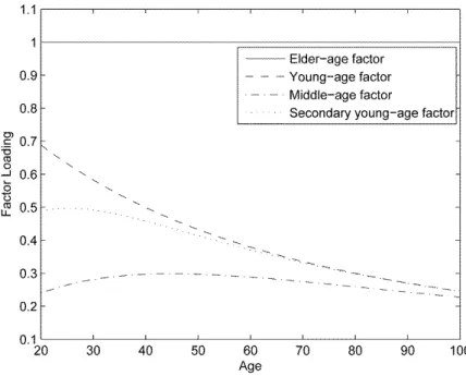
1,…,6, being used to capture the period effect. Each of the exponential components can be seen as reflecting the degree of sensitivity of the mortality curve to a particular factor; hence, the term ‘factor loadings’. These components, referred to by the age region in which the factor loading has the highest value (i.e., where it is most sensitive to the factor movement), are illustrated in Figure 1 as a function of age.
The ‘young-age’ component has the highest value in the youngest age group, which can be seen from the term (1 − 𝑒−𝜆1𝑥)/(𝜆1𝑥), where it initially shows the greatest value in
the youngest age group, and then starts to decay monotonically at a speed controlled by the decay parameter λ1. The ‘middle-age’ factor loading (1 − 𝑒−𝜆1𝑥)/(𝜆1𝑥) − 𝑒−𝜆1𝑥 is a
hump-shaped function which reaches its maximum value during middle age, where the location of the maximum is again determined by the value of λ1. The ‘elder-age’ factor
loading is a constant of all ages and is therefore found to be dominant amongst the elder age groups. An additional component (1 − 𝑒−𝜆1𝑥)/(𝜆1𝑥) − 𝑒−2𝜆1𝑥 is also presented in order
to capture the small, but frequent, variations amongst the younger age groups.
For the purpose of flexibility, two pairs of factor loadings are specified within the model, each with different decay parameters, λ1 and λ2. By adjusting the value of the decay
parameter (λi), the factor loadings reflect the different behavior patterns of the age effect, as
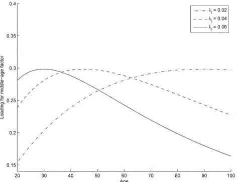
shown in Figures 2 and 3. In the ‘young-age’ factor loading, the decay parameter determines the speed of decay in terms of sensitivity to the period effect. As shown in Figure 2, a larger value of λi indicates a more rapid decay in the factor loading value with an increase in age.
In Figure 3, the decay parameter also controls the speed of the decay in the middle-age factor loading, with a larger λi implying a larger hump in the middle-age factor loading.
<Figures 2 and 3 are inserted about here>
The period effect is explained by the factors βt = [β1t, β2t, β3t, β4t, β5t, β6t]′, which are the
drivers determining the evolution of the mortality rate curves across different periods. As noted by Diebold and Li (2006), these factors can be seen as dynamic latent factors governed by time-series models; in specific terms, each of the factors represents the forces governing the evolution of the mortality curve, with the factor loadings representing the sensitivity of the mortality curve to such forces.
We can forecast these factors by selecting an appropriate time-series model and then obtain a forecast of the mortality curve by recombining the forecasted factors with their associated factor loadings. If each factor is assumed to be Gaussian, then the mortality rate becomes a Gaussian random variable, in which case, the density forecast can be obtained.
2.2 The Lee-Carter Model
The original version of the Lee-Carter model takes the following form:
log 𝑚(𝑥, 𝑡) = 𝑎𝑥+ 𝑏𝑥𝑘𝑡+ 𝜀𝑥,𝑡 . (2)
where the central death rate for each age x at time t, m(x,t), is associated with a base parameter ax and an additional parameter, bx, which together describe the age effect; the ax
and bx parameters are also referred to as the ‘age-specific constant’, essentially because they
relate only to age, and also because once they are estimated, they are fixed. The kt variable
alone captures the period effect.
Although the Lee-Carter model has been widely adopted in numerous prior studies, and with some empirical success, it does have some weaknesses which are essentially based upon
its simplicity. Criticism is often directed at the single factor (kt) setting of the model, which
raises two major concerns; firstly, a single source of time variation implies that all shocks to mortality rates are perfectly correlated over time; and secondly, the invariant bx under the
single source of time variation restricts changes in the mortality rates to the relative magnitudes of bx (Girosi and King, 2007). An additional concern is the distinct lack of
smoothness in the mortality curve produced by the Lee-Carter model due to the fact that bx is
unconstrained.
Our approach provides improvements upon the Lee-Carter benchmark model from two aspects. These theoretical advantages are illustrated in Equations (3) to (6), where both the Lee-Carter model and our six-factor model (with the age subscripts suppressed) are expressed as:
𝐿𝐶: log 𝑚(𝑡) = 𝑎 + 𝑏𝑘𝑡+ 𝜀𝑡 (3)
𝑘𝑡 = 𝜃 + 𝑘𝑡−1+ 𝑣𝑡 (4)
6𝐹: log 𝑚(𝑡) = 𝑋β𝑡+ 𝜇𝑡 (5)
𝛽𝑡= 𝛿 + 𝛽𝑡−1+ 𝜂𝑡 (6)
where log m(t) denotes the log mortality curve in year t; a and b are the vectors of ax and bx in the Lee-Carter model, θ is a scalar drift for kt, X is the matrix of the factor loadings, δ is the drift vector for βt, and βt represents the factors in year t. According to Girosi and King (2007), both models may be further rewritten as: 𝐿𝐶: log 𝑚(𝑡) = log 𝑚(𝑡 − 1) + 𝜃𝑏 + (𝑏𝑣𝑡+ 𝜀𝑡− 𝜀𝑡−1) (7)
6𝐹: log 𝑚(𝑡) = log 𝑚(𝑡 − 1) + 𝑋𝛿 + (𝑋𝜂𝑡+ 𝜇𝑡− 𝜇𝑡−1) (8)
The error terms are essentially restrictions on the covariance matrices implied by both models. Mortality in the Lee-Carter model is subject to only two shocks: bvt that is perfectly
correlated across all ages and εt being uncorrelated across different ages. Conversely, our
six-factor model exhibits multiple sources of shocks from the different factors across various ages. The more flexible correlation structure of Equation (8) is obtained by simultaenously considering multiple evolutions in mortality trends, as opposed to single evolution.
3. IN-SAMPLE ESTIMATIONS
3.1 Parameter Estimation
We estimate our six-factor model using a two-stage procedure, with the first stage involving the determination of the decay parameters, λ = [λ1, λ2], by minimizing the quadratic
estimation error in the log mortality curve. The second stage involves the use of the OLS method to estimate the βt factors, based upon the λ determined in the first stage. The first
min𝛌 ∑ 𝑋,𝑇𝑥,𝑡 (log 𝑚(𝑥, 𝑡) − log 𝑚�(𝑥, 𝑡, β𝑡(λ)))2
s. t. λ1− λ2 ≥ c, c ∈ ℝ (9)
where X and T are the last age and period in the sample. Once the optimized values of λ* = [𝜆1∗, 𝜆2∗] have been determined, Equation (1) immediately becomes linear in βt; that is, plug
in λ* into factor loading X in Equation (5) to have:
log 𝑚�(𝑥, 𝑡, β𝑡(λ∗)) = 𝑋∗β𝑡. (10)
We can then obtain βt in the second stage using the standard OLS technique and enter the
OLS estimate back into the first stage to calculate the estimation error.
Prior to commencing with the first stage estimation, we must specify a set of constraints for the ranges of λ to avoid problems that may arise from inappropriate values of λ. A poorly specified λ would result in a failure to identify the components and multicollinearity amongst the components (Bolder and Streliski, 1999; de Pooter, 2007).
To avoid the potential numerical problem referred to above, we follow Gilli, Grosse and Schumann (2010), in which it was suggested that a restriction should be placed upon the value of λ based upon the correlations between the factor loadings; we therefore set the boundary of λ at [0.0291,0.0414]. Given the value of the decay parameter, we can calculate the correlation between the two factor loadings. We restrict the correlation between the ‘young-age’ and ‘middle-age’ factor loading to [–0.7, 0.7]. The limit is chosen to be below the level of ‘highly correlated’ from standard advice of statistic textbook.
A second constraint is then imposed on the minimum distance between λ1 and λ2; this
constraint is λ1– λ2>0.0037. The minimum distance constraint for λ controls the distance
between the two factor loadings, an approach proposed by de Pooter (2007) as a means of further alleviating the potential risk of multicollinearity between the factor loadings. In the extreme case where the two decay parameters are equal, the six-factor model would degenerate to a four-factor one and result in numerically inaccurate parameter estimates.
In order to avoid such a case, we set a minimum distance of five years between the ages where the maximum loading appears for two middle-age factors; this implied minimum difference between λ1 and λ2 is set at 0.0037 by a simple grid search within the
implied boundary of λ. Given this boundary for λ, the maximum value for middle-age factor loadings would appear between the ages of 43 and 62, thereby providing a good fit for our purpose of describing the middle-age mortality rate.1
3.2 Data Description and Accuracy Measure
1
The location of the maximum loading provides a good reflection of the location of the curl on the mortality rate curve. The bend points for two middle-age factor loadings should not be too close, otherwise multicollinearity will be found to exist between the middle-age factor loadings. Although the selection of five years as the minimum distance was an ad hoc choice, further tests were carried out using three and seven years in order to provide a test for robustness, with the results showing that the forecasting performance remained intact with these alternative choices.
Our empirical tests on the two competing models were performed using the central death rates for ages from 20 to 100 obtained from the Human Mortality Database (2011). Samples were obtained for every country for which mortality data during the post-1950 period were available, including both male and female populations within our sample. The sample period for each country was determined by the last mortality rate available within the database.2
<Table 1 is inserted about here> The 23 countries in our sample are listed in Table 1.
Two accuracy measures, root mean square error (RMSE) and mean absolute error (MAE), are used in this study to evaluate model fitness. RMSE imposes heavier penalties on greater errors by squaring the errors, whilst MAE focuses on the average of the absolute errors. The measures for each fitting period, t, are computed as:
RMSE(𝑡) = �N1∑𝑥𝑁
𝑥=𝑥1 (log 𝑚(𝑥, 𝑡) − log 𝑚�(𝑥, 𝑡))2 (11)
MAE(𝑡) =N1∑𝑥N
𝑥=𝑥1 |log 𝑚(𝑥, 𝑡) − log 𝑚�(𝑥, 𝑡)| (12)
where 𝑚(𝑥, 𝑡) is the observed (actual) central death rate of age x = x1, …, xN in year t, and
𝑚�(𝑥, 𝑡) is the fitted or forecasted value obtained from the model, with a greater RMSE or MAE indicating greater estimation errors. We then calculate the improvement ratios for the above measures defined as the RMSE of our model over the RMSE of the Lee-Carter benchmark model, thereby providing a direct comparison of in-sample fitting and out-of-sample forecasting performance, as follows:
RMSE improvement ratio = 1 −�∑
𝑇
𝑡=1∑𝑥𝑁𝑥=𝑥1(log 𝑚(𝑥,𝑡)−log𝑚�6𝐹(𝑥,𝑡))2
�∑𝑇
𝑡=1∑𝑥𝑛𝑥=𝑥0(log 𝑚(𝑥,𝑡)−log𝑚�𝐿𝐶(𝑥,𝑡))2
(13)
MAE improvement ratio = 1 −∑𝑇𝑡=1∑𝑥𝑁𝑥=𝑥1|log 𝑚(𝑥,𝑡)−log𝑚�6𝐹(𝑥,𝑡)|
∑𝑇
𝑡=1∑𝑥𝑁𝑥=𝑥1|log 𝑚(𝑥,𝑡)−log𝑚�𝐿𝐶(𝑥,𝑡)| (14)
where T denotes the data period, x1 denotes the initial age, and xN denotes the last age within
the data. A positive ratio would indicate that our six-factor model had produced a more accurate forecast.
3.3 Fitting Results
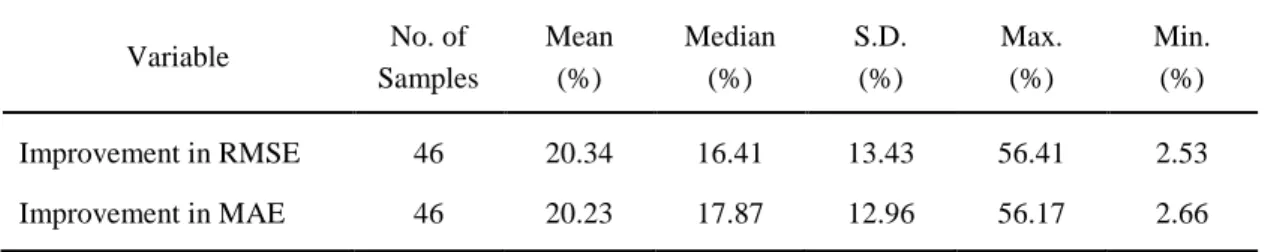
The results shown in Table 2 reveal that our model fits worldwide mortality curves better than the Lee-Carter model, with average (median) improvement ratios across the sampled countries of 20.3 percent (16.4 percent) for RMSE, and 20.2 percent (17.9 percent) for
2
The sample for Iceland was ultimately excluded from this study because it contained too many zero mortality rates which resulted in numerical inconsistencies within the estimations of both the Lee-Carter model and our six-factor model.
MAE . The maximum improvement in RMSE is found for female mortality in Japan, at 56.4 percent, whilst the minimum improvement is found for female mortality in the Netherlands, at 2.5 percent; similar results are also reported for MAE. These comparison results suggest that our model has superior fitting performance in all of the sampled contries.
<Table 2 is inserted about here>
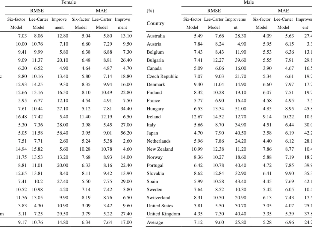
As shown in Table 3, in terms of both RMSE and MAE, our six-factor model is found to produce a better fit for female mortality across all 23 countries. The average RMSE (MAE) for the six-factor model was found to be 9.17 percent (6.34 percent), whilst that for the Lee-Carter model was found to be 10.76 percent (7.64 percent). Table 3 also indicate the efficacy of our six-factor model with regard to male mortality. For instance, our model prevails in all male populations in terms of RMSE, with an average of 7.12 percent versus the 9.60 percent of the Lee-Carter model. The resulting improvement ratio for RMSE is reaching 26 percent, almost twice as much as that found for the female mortality curves (15 percent). Improvement ratios in excess of 40 percent are discernible for Bulgaria, Japan, Portugal, Spain and the United Kingdom. As regards performance for different gender samples, both the six-factor model and the Lee-Carter model demonstrate better fitting performance on male data than on female data.
<Table 3 is inserted about here>
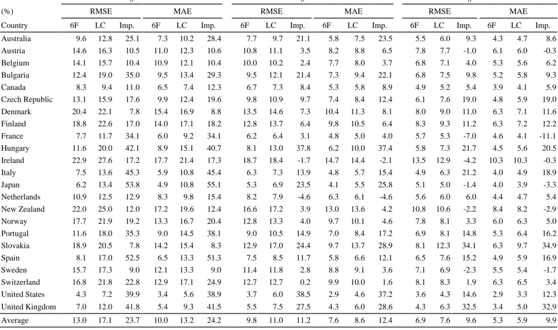
The samples were then categorized into six age groups: 20-34 years, 35-44 years, 45-64 years, 65-74 years, 75-84 years and 85-100 years, with Table 4 reporting the results. The figures shown in the ‘Average’ row in Table 4 demonstrate that across the different age groups, our model invariably provides better fitting performance than the Lee-Carter model worldwidely. Furthermore, our model dominate 86 percent of the cases in terms of RMSE and MAE.
<Table 4 is inserted about here>
With regard to the fitting to each age group, the average improvement ratio is found to be 23.7 percent and 24.2 percent, in term of RMSE and MAE for the 20-34 age group. Our model provides more accurate estimate for every country in the age group of 20-34. Within the 35-44 group, the estimate of our model is more accurate in 21 countries in terms of both RMSE and MAE; similar comparisons on the age 45-64 group suggest that our model is more accurate in 17 countries. The average improvement ratios for MAE were 18.00 percent in the 65-74 age group, 33.70 percent in the 75-84 age group, and 28.10 percent in the 85-100 age group. There are 15 countries favoring our model in the 65-74 age group, 22 countries in the 75-84 age group, and 20 countries in the 85-100 age group. Similar advantages of our model relative to the Lee-Carter model can be found even we switch the accuracy measure to RMSE. Our model has a clear comparative advantage in the older age groups, which is important since these groups are considered to be the primary source of longevity risk.
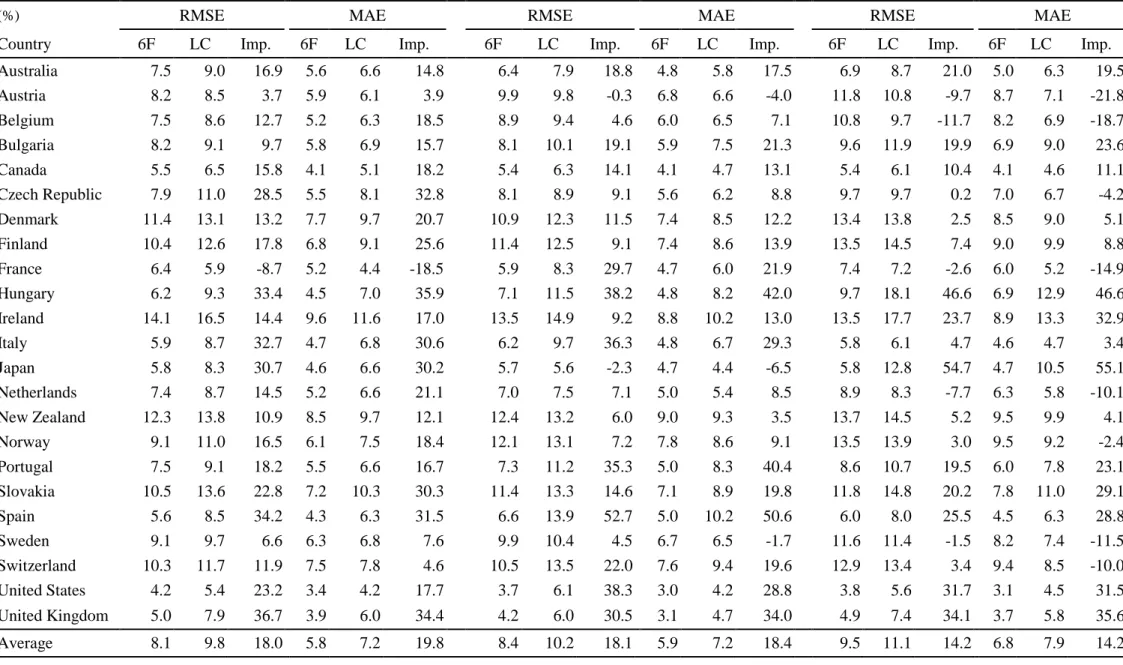
For further robustness check, the sampling periods were subsequently split into six decade groups: the 1950s, 1960s, 1970s, 1980s, 1990s and 2000s, with Table 5 showing that
the fitting accuracy of our model is consistently better across each of these periods. Throughout all six periods, our model outperform in 14 of the 23 countries, with the most significant performances being discernible for Japan, Hungary, the United Kingdom and Spain. Among all decade groups, the best relative performance is found in the 1950s. We speculate that in the 1950s, the mortality curves of some countries were still subject to the effects of World War II, and hence, irregular patterns are demonstrated. The flexibility of our model appears to be sufficient in capturing the irregular patterns during that particular period. The results from the are similar for each period, with our six-factor model demonstrating improvements of around 18 percent in the RMSE ratios. In the periods from 1960s to the 1990s, our model is found to have both a lower RMSE and a lower MAE for almost all countries. In the 2000s, our model reveals an average improvement ratio of 14.2 percent.
<Table 5 is inserted about here>
4. OUT-OF-SAMPLE FORECASTING
4.1 Forecasting Procedure
The forecasting procedure beginning with the application of the two-stage estimation of the parameter, λ, and the factor, βt, as described in the previous section. After obtaining the
forecasted values of these factors, they are re-entered into Equation (1), along with the associated λ, in order to project the mortality rate curves.
We adopt the random walk with drift (RWD) model for the individual factors for two reasons. Firstly, although the usual augmented Dickey-Fuller test and Box-Jenkin procedure should be applied to the factors in order to select the best model, in practice, we sometimes find that the use of different time-series models for each of the factors may lead to inconsistent forecasting. We therefore select the RWD model to simplify the procedure and achieve greater consistency.3
Secondly, in order to compare the effects of the modeling trade-off between the age and period effects, we need to control the time-series model at the very least so as to maintain comparable grounds. The mortality trend, kt, in the Lee-Carter model has produced
empirically accurate forecasting in the past, an example of which is provided by Tuljapurkar et al. (2000). Furthermore, it is well known that mortality rates show declining trends across countries and age groups during the post-war period, which also suggests that the RWD model may be an appropriate choice.
The window used in the first-stage estimation is set at 30 years in order to ensure that an adequate number of samples is reserved for model construction. This also ensures that sufficient numbers of unused observation are available for use in the forecasting tests. The
3
A similar approach was also adopted by Lee and Carter (1992); according to their findings, “a similar model with an ar(1) term added was marginally superior, but we preferred the (0,1,0) model on grounds of parsimony” (pp.669).
first estimation window runs from 1950 to 1979, with the window then rolling forward by a one-year step, such that the second estimation period runs from 1951 to 1980, and so on; 1-, 3-, 5-, 10- and 15-year factor forecasts are then generated for each of these rolling windows. We repeat these forecasting procedures for at least 27 rounds for the 1-year forecast horizon, 25 rounds for the 3-year forecasts, 23 rounds for the 5-year forecasts, and so on, depending upon the overall duration of the data available for each of the countries.
4.2 Forecasting Results
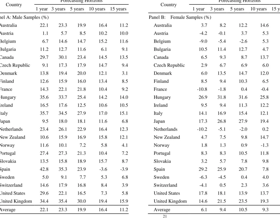
Our initial assessment of relative forecasting performance is undertaken from the aspect of gender. As we can see from the comparisons of the male mortality samples in Panel A of Table 6, our six-factor model dominates in almost all of the RMSE improvement ratios. Out of the 115 comparisons (23 countries x 5 forecasting periods), our model was found to outperform the Lee-Carter model in 110 rounds (i.e., 96 percent of the time). Given the broad range of our sample, the average improving magnitude across the various forecasting periods is found to be quite significant; the average improvement ratio of 1-, 3-, 5-, 10- and 15-year forecasting horizons are 19.9 percent, 20.2 percent, 17.1 percent, 10.0 percent and 6.80 percent, with an overall average improvement ratio of 14.8 percent.
<Table 6 is inserted about here>
The improvement ratios in RMSE for female mortality are reported in Panel B of Table 6, from which we can see that our model dominates in 88 percent of all cases. The average improvement ratios of 1-, 3-, 5-, 10- and 15-year forecasting horizons are 7.5 percent, 9.5 percent, 9.4 percent, 8.1 percent and 7.3 percent, with an overall average improvement ratio of 8.4 percent. It is clear that our model provides more accurate forecasting of both male and female mortality rates, with the improvements over the Lee-Carter model being found to be more significant for male mortality rates. The improvements in MAE for different horizons largely resemble those already found with regard to RMSE.
The last rows of Table 6 show that the greatest improvement ratios are found in the 3-year forecasting horizons. The improvements then decline with the forecasting horizon, which may be attributable to the small number of factors used to depict the overall dynamics of the entire mortality rate curves. Erratic changes may be discernible with a lengthening of the forecasting horizon; In addition, sudden structural changes may arise to which the RWD drift is unable to respond as noted by Coelho and Nunes (2011). Nevertheless, as long as life insurers carry out periodic dynamic hedging on the mortality rate risk, this inherent ‘weakness’ of our model will disappear.
4.3 The Panel Diebold-Mariano Test
Notwithstanding the evidence already presented, we cannot reject the ‘equal accuracy’ hypothesis without carrying out a statistical test. We conduct a panel Diebold-Mariano (DM) test which was developed by Pesaran, Schuermann and Smith (2009) to examine same- age time-series panel data across different countries – to determine whether the improvements
of our model over the Lee-Carter model is statistically significant.4
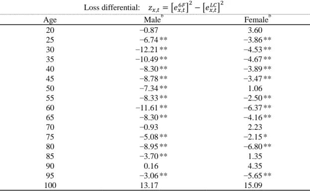
𝑧(𝑥, 𝑡) = [𝑒6𝐹(𝑥, 𝑡)]2− [𝑒𝐿𝐶(𝑥, 𝑡)]2 (15)
Following Diebold and Mariano (1995), the loss differential in the mortality rates is defined as:
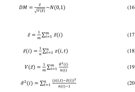
where e6F(x,t) and eLC(x,t) are the respective one-year ahead forecast error terms in our six factor model and the Lee-Carter model; xrefers to age (in years); and t = 1, …, n refers to the calendar year of the forecast. We pick out every other five age starting from age 20 to test the accuracy of mortality forecast. The panel DM test statistic was derived by Pesaran et al. (2009) as follows: 𝐷𝑀 =�𝑉(𝑧̅)𝑧̅ ~𝑁(0,1) (16) where 𝑧̅ =𝑚1∑𝑚 𝑖=1 𝑧̅(𝑖) (17) 𝑧̅(𝑖) =1𝑛∑𝑛 𝑡=1𝑧(𝑖, 𝑡) (18) 𝑉(𝑧̅) = 𝑚1 ∑𝑚 𝑖=1 𝜎� 2(𝑖) 𝑛(𝑖) (19) 𝜎�2(𝑖) = ∑𝑛 𝑡=1 (𝑧(𝑖,𝑡)−𝑧̅(𝑖)) 2 𝑛(𝑖)−1 (20)
and where the number of countries is denoted as i = 1, …, 23. A negative DM test statistic would indicate the better forecasting of our model over the Lee-Carter model.5
The results are reported in Table 8. We can see that almost all of the DM statistics are negative and significant at the 95 percent confidence level, thereby suggesting that as compared to the Lee-Carter model, our six-factor model produces more accurate forecasting for different age groups and across different countries.
<Table 8 is inserted about here>
Table 8 also suggests that our model is significantly better at profiling the younger aged mortality. From age 25 to age 65, the DM statistics of both male and female population became significantly negative and rejected the null hypothesis except age 50 in female population. For age above 85, the DM statistics show that our projection is more accurate
4
Also available to us is the possibility of examining the forecasting errors within each country and then carrying out the original DM test across different ages; however, the problem with this approach is that the forecasted series has only limited length, and any statistical tests using small samples will not be convincing. Thus, the panel DM test, involving comparisons of the forecasting accuracy of the two models for individual age mortality rates, using our comprehensive panel dataset, is more appealing.
5
Pesaran et al. (2009) noted that there was potential serial autocorrelation in the loss differential, a problem which could be dealt with using the HAC estimator. Another concern is that the DM statistic may no longer be asymptotic to standard normal distribution if the cross-section dependence is significant and the number of forecasts is small; we therefore go on to compute Newey-West variance with a maximum lag equal to 1, and find that the results are similar.
for male mortality. A possible explanation for the better fitting on the younger aged mortality is that the oldest mortality estimates in our model tend to converge to the elder-age factor (β0),
with the estimated mortality rates at the very end being prone to changes in the elder-age in our model. Furthermore, with a decline in the effects of the other factors, the elder-age factor alone cannot accurately describe the end-point mortality rate.
5. CONCLUSIONS
We analyze the applicability of two different mortality modeling strategies to worldwide cases in the present study: a curve-fitting approach and the widely adopted Lee-Carter model. The major contributions of our approach are the parsimonious age effect, the feasibility of interpolation, and an analytical tractable function form. Mortality curve forecasting in our approach is built upon linear, additive factors, where each of the factors is projected by a random walk with drift model.
We carried out a large-scale comparison using mortality data on 46 gender-specific populations. Tthe results indicate that our approach significantly outperforms the standard benchmark approach, in both in-sample fitting and out-of-sample forecasting. We subsequently carried out a panel Diebold-Mariano (DM) test to determine statsitical significance of the improvement of our model over the Lee-Carter model. The results validated the improvements found in most of the sample populations. We can therefore conclude that our model is capable of producing more accurate forecasting of the adult mortality curve than the Lee-Carter model.
REFERENCES
Bolder, D.J. and D. Streliski (1999), ‘Yield Curve Modelling at the Bank of Canada’, Technical Report, Bank of Canada.
Coelho, E. and L.C. Nunes (2011), ‘Forecasting Mortality in the Event of a Structural Change’, Journal of the Royal Statistical Society: Series A (Statistics in Society), 174(3): 713-36.
de Pooter, M. (2007), ‘Examining the Nelson-Siegel Class of Term Structure Models’, Tinbergen Institute Discussion Paper 07-043/4, Tinbergen Institute.
Diebold, F.X. and C. Li (2006), ‘Forecasting the Term Structure of Government Bond Yields’,
Journal of Econometrics, 130(2): 337-64.
Diebold, F.X. and R.S. Mariano (1995), ‘Comparing Predictive Accuracy’, Journal of
Business & Economic Statistics, 13(5): 253-63.
Gilli, M., S. Grosse and E. Schumann (2010), ‘Calibrating the Nelson-Siegel-Svensson Model’, Technical Report 31, COMISEF Working Papers Series.
Girosi, F. and G. King (2007), ‘Understanding the Lee-Carter Mortality Forecasting Method’, Technical Report, RAND Corporation.
Human Mortality Database (2011), The Human Mortality Database, University of California, Berkeley (USA) and the Max Planck Institute for Demographic Research (Germany), data accessed on 20 June 2011.
Lee, R. and L. Carter (1992), ‘Modeling and Forecasting US Mortality’, Journal of the
American Statistical Association, 87(419): 659-75.
Nelson, C. and A. Siegel (1987), ‘Parsimonious Modeling of Yield Curves’, Journal of
Business, 60(4): 473-89.
Pesaran, M.H., T. Schuermann and L.V. Smith (2009), ‘Forecasting Economic and Financial Variables with Global VARs’, International Journal of Forecasting, 25(4):642-75. Tuljapurkar, S., N. Li and C. Boe (2000), ‘A Universal Pattern of Mortality Decline in the G7
Figure 1 Factor loadings for different age components
Note: This figure illustrates the four distinct components in the six-factor model, with each
of the components (factors) being referred to as the age region at which the sensitivity (factor loading) is the highest.
Figure 2 Changes in young-age factor loading with decay parameter λi, i =1,2 Note: This figure illustrates the variations in the young-age factor loading values at different
ages, given three different decay parameter values, with the weighting of each age relative to the young-age factor being determined by the value of the factor loading. The decay parameter controls the speed at which the value of the factor loading decreases with age.
Figure 3 Changes in middle-age factor loading with decay parameter λi, i =1,2 Note: This figure illustrates the variations in the middle-age factor loading values at different
ages, given three different decay parameter values, with the weighting of each age relative to the middle-age factor being determined by the value of the factor loading. The decay parameter controls the location of the ‘hump’ in the factor loading, the point at which nearby ages are most sensitive to the middle-age factor.
Table 1 Sample countries from the Human Mortality Database (n = 23)
Geographical Region
(No. of Countries) Country Sample Period
Asia-Pacific (3)
Australia 1950-2007
New Zealand 1950-2008
Japan 1950-2009
Europe (18)
Hungary; Ireland; Spain 1950-2006
France; Italy; Switzerland 1950-2007
Austria; Denmark; Netherlands;
Norway; Sweden; 1950-2008
Belgium; Bulgaria; Czech Republic; Finland; Portugal; Slovakia; United Kingdom
1950-2009
North America (2) Canada; United States 1950-2007
Table 2 Descriptive statistics on improvement ratios of the six-factor model versus the Lee-Carter model across 46 gender-country populations
Variable No. of Samples Mean (%) Median (%) S.D. (%) Max. (%) Min. (%) Improvement in RMSE 46 20.34 16.41 13.43 56.41 2.53 Improvement in MAE 46 20.23 17.87 12.96 56.17 2.66
Table 3 In-sample fitting performance, by genders
Female Male
(%) RMSE MAE (%) RMSE MAE
Country Six-factor Model Lee-Carter Model Improve ment Six-factor Model Lee-Carter Model Improve ment Country Six-factor Model Lee-Carter Model Improveme nt Six-factor Model Lee-Carter Model Improvem ent Australia 7.03 8.06 12.80 5.04 5.80 13.10 Australia 5.49 7.66 28.30 4.09 5.63 27.40 Austria 10.00 10.76 7.10 6.60 7.29 9.50 Austria 7.84 8.24 4.90 5.95 6.15 3.30 Belgium 9.41 9.99 5.80 6.38 6.88 7.30 Belgium 7.43 8.43 11.90 5.53 6.36 13.10 Bulgaria 9.09 11.37 20.10 6.48 8.81 26.40 Bulgaria 7.41 12.27 39.60 5.55 7.91 29.80 Canada 6.20 6.52 4.90 4.64 4.87 4.70 Canada 5.09 6.06 16.00 3.90 4.67 16.50 Czech Republic 8.80 10.16 13.40 5.80 7.14 18.80 Czech Republic 7.07 9.03 21.70 5.34 6.61 19.20 Denmark 12.93 14.25 9.30 8.35 9.94 16.00 Denmark 9.40 11.04 14.90 6.60 7.97 17.20 Finland 12.66 15.16 16.50 8.10 10.49 22.80 Finland 8.32 10.28 19.10 6.07 7.51 19.20 France 5.95 6.77 12.10 4.54 4.91 7.50 France 5.77 6.90 16.40 4.58 4.95 7.50 Hungary 7.61 10.44 27.10 5.12 7.81 34.40 Hungary 6.53 13.34 51.00 4.85 8.95 45.80 Ireland 16.48 17.42 5.40 11.40 12.19 6.50 Ireland 12.67 14.52 12.70 9.14 10.22 10.60 Italy 5.30 7.36 28.00 3.98 5.45 27.00 Italy 5.66 8.70 34.90 4.51 6.44 30.00 Japan 5.05 11.58 56.40 3.95 9.01 56.20 Japan 4.70 7.90 40.50 3.58 6.19 42.20 Netherlands 7.51 7.71 2.60 5.24 5.38 2.60 Netherlands 5.96 7.86 24.20 4.40 6.12 28.10 New Zealand 14.94 15.82 5.60 10.28 10.78 4.60 New Zealand 10.99 12.38 11.20 7.86 8.77 10.40 Norway 11.75 13.53 13.20 7.68 8.93 14.00 Norway 8.36 10.27 18.60 5.88 7.19 18.20 Portugal 8.81 11.01 20.00 6.33 8.16 22.40 Portugal 6.42 10.78 40.40 4.72 7.85 39.90 Slovakia 12.65 13.81 8.40 8.11 9.42 13.90 Slovakia 8.62 12.84 32.90 6.41 9.90 35.30 Spain 7.41 10.2 27.40 5.50 7.75 29.00 Spain 5.99 10.58 43.40 4.45 7.69 42.10 Sweden 10.52 10.98 4.20 7.14 7.42 3.80 Sweden 7.64 8.52 10.30 5.42 6.05 10.40 Switzerland 11.76 13.05 9.90 8.19 8.76 6.50 Switzerland 8.31 10.50 20.90 6.13 7.43 17.50 United States 3.83 4.30 10.90 3.09 3.42 9.60 United States 3.81 5.50 30.70 3.05 4.07 25.10 United Kingdom 5.11 7.25 29.50 3.79 5.22 27.40 United Kingdom 4.35 7.30 40.40 3.35 5.39 37.80 Average 9.17 10.76 14.80 6.34 7.64 17.00 Average 7.12 9.60 25.80 5.28 6.96 24.20
Table 4 In-sample fitting performance, by age groups
Age 20-34 Age 35-44 Age 45-64
(%) RMSE MAE RMSE MAE RMSE MAE
Country 6F LC Imp. 6F LC Imp. 6F LC Imp. 6F LC Imp. 6F LC Imp. 6F LC Imp. Australia 9.6 12.8 25.1 7.3 10.2 28.4 7.7 9.7 21.1 5.8 7.5 23.5 5.5 6.0 9.3 4.3 4.7 8.6 Austria 14.6 16.3 10.5 11.0 12.3 10.6 10.8 11.1 3.5 8.2 8.8 6.5 7.8 7.7 -1.0 6.1 6.0 -0.3 Belgium 14.1 15.7 10.4 10.9 12.1 10.4 10.0 10.2 2.4 7.7 8.0 3.7 6.8 7.1 4.0 5.3 5.6 6.2 Bulgaria 12.4 19.0 35.0 9.5 13.4 29.3 9.5 12.1 21.4 7.3 9.4 22.1 6.8 7.5 9.8 5.2 5.8 9.3 Canada 8.3 9.4 11.0 6.5 7.4 12.3 6.7 7.3 8.4 5.3 5.8 8.9 4.9 5.2 5.4 3.9 4.1 5.9 Czech Republic 13.1 15.9 17.6 9.9 12.4 19.6 9.8 10.9 9.7 7.4 8.4 12.4 6.1 7.6 19.0 4.8 5.9 19.0 Denmark 20.4 22.1 7.8 15.4 16.9 8.8 13.5 14.6 7.3 10.4 11.3 8.1 8.0 9.0 11.0 6.3 7.1 11.6 Finland 18.8 22.6 17.0 14.0 17.1 18.2 12.8 13.7 6.4 9.8 10.5 6.4 8.3 9.3 11.2 6.3 7.2 12.2 France 7.7 11.7 34.1 6.0 9.2 34.1 6.2 6.4 3.1 4.8 5.0 4.0 5.7 5.3 -7.0 4.6 4.1 -11.1 Hungary 11.6 20.0 42.1 8.9 15.1 40.7 8.1 13.0 37.8 6.2 10.0 37.4 5.8 7.3 21.7 4.5 5.6 20.5 Ireland 22.9 27.6 17.2 17.7 21.4 17.3 18.7 18.4 -1.7 14.7 14.4 -2.1 13.5 12.9 -4.2 10.3 10.3 -0.3 Italy 7.5 13.6 45.3 5.9 10.8 45.4 6.3 7.3 13.9 4.8 5.7 15.4 4.9 6.3 21.2 4.0 4.9 18.9 Japan 6.2 13.4 53.8 4.9 10.8 55.1 5.3 6.9 23.5 4.1 5.5 25.8 5.1 5.0 -1.4 4.0 3.9 -3.3 Netherlands 10.9 12.5 12.9 8.3 9.8 15.4 8.2 7.9 -4.6 6.3 6.1 -4.6 5.6 6.0 6.0 4.4 4.7 5.4 New Zealand 22.0 25.0 12.0 17.2 19.6 12.4 16.6 17.2 3.9 13.0 13.6 4.2 10.8 10.6 -2.2 8.4 8.2 -2.9 Norway 17.7 21.9 19.2 13.3 16.7 20.4 12.8 13.3 4.0 9.7 10.1 4.6 7.8 8.1 3.3 6.0 6.3 5.0 Portugal 11.6 18.0 35.3 9.0 14.5 38.1 9.0 10.5 14.9 7.0 8.4 17.2 6.9 8.1 14.8 5.3 6.4 16.2 Slovakia 18.9 20.5 7.8 14.2 15.4 8.3 12.9 17.0 24.4 9.7 13.7 28.9 8.1 12.3 34.1 6.3 9.7 34.9 Spain 8.1 17.0 52.5 6.5 13.3 51.3 7.5 8.5 11.7 5.8 6.6 12.1 6.5 7.6 15.2 4.9 5.9 16.9 Sweden 15.7 17.3 9.0 12.1 13.3 9.0 11.4 11.8 2.8 8.8 9.1 3.6 7.1 6.9 -2.3 5.5 5.4 -1.7 Switzerland 16.8 21.8 22.8 12.9 17.1 24.9 12.7 12.7 0.2 9.9 10.0 1.6 8.1 8.3 1.9 6.3 6.5 3.4 United States 4.3 7.2 39.9 3.4 5.6 38.9 3.7 6.0 38.5 2.9 4.6 37.2 3.6 4.3 14.6 2.9 3.3 12.3 United Kingdom 7.0 12.0 41.8 5.4 9.3 41.5 5.5 7.5 27.5 4.3 6.0 28.6 4.3 6.3 32.5 3.4 5.0 32.9 Average 13.0 17.1 23.7 10.0 13.2 24.2 9.8 11.0 11.2 7.6 8.6 12.4 6.9 7.6 9.6 5.3 5.9 9.9
Table 4 (Cont. )
Age 65-74 Age 75-84 Age 85-100
(%) RMSE MAE RMSE MAE RMSE MAE
Country 6F LC Imp. 6F LC Imp. 6F LC Imp. 6F LC Imp. 6F LC Imp. 6F LC Imp. Australia 4.8 4.8 -0.6 3.7 3.8 3.1 3.9 4.0 3.3 3.0 3.3 6.5 4.2 5.6 24.8 3.1 4.4 29.2 Austria 6.1 6.1 0.2 4.7 4.9 3.7 4.2 5.2 20.0 3.3 4.2 20.8 5.3 5.0 -5.8 3.8 3.8 0.0 Belgium 5.8 6.6 11.5 4.5 5.2 13.2 3.8 5.4 28.4 3.0 4.2 28.1 5.4 5.5 2.2 3.9 4.3 9.4 Bulgaria 6.3 8.8 29.2 4.8 7.0 31.4 6.2 8.8 29.2 4.7 7.1 33.3 6.5 10.5 38.1 4.5 7.9 42.9 Canada 4.5 4.3 -5.1 3.6 3.4 -6.8 3.4 4.2 17.9 2.7 3.4 18.2 4.4 5.3 17.7 3.4 4.3 19.8 Czech Republic 5.3 6.9 22.6 4.2 5.2 19.7 4.2 6.6 35.9 3.3 5.2 36.8 5.1 5.4 5.5 3.6 4.1 11.5 Denmark 5.7 7.4 23.0 4.4 5.9 24.8 4.3 7.4 41.8 3.5 6.0 42.5 5.6 7.8 29.0 4.1 6.2 32.7 Finland 6.0 9.1 33.3 4.7 7.1 34.1 5.0 8.5 41.3 3.8 6.4 40.7 4.9 6.9 29.0 3.4 5.5 38.6 France 5.8 4.9 -19.7 4.8 3.8 -25.7 3.7 4.9 24.5 2.9 3.8 24.4 4.9 4.2 -17.7 3.9 3.3 -18.3 Hungary 4.7 6.9 32.2 3.6 5.5 35.1 4.3 9.3 53.9 3.2 7.5 57.2 4.6 9.6 52.5 3.2 7.0 54.5 Ireland 10.3 11.1 7.5 7.8 9.0 13.3 9.3 8.2 -13.5 7.0 6.5 -7.2 6.1 6.8 9.9 4.2 5.2 20.0 Italy 5.4 6.1 12.1 4.5 5.0 11.2 3.7 6.1 39.4 2.9 5.0 41.8 4.3 5.1 14.5 3.4 4.0 16.6 Japan 4.7 9.2 48.4 3.9 7.2 45.9 2.9 13.2 77.8 2.4 11.2 78.6 3.9 10.4 62.1 3.0 8.5 64.9 Netherlands 4.6 6.2 25.3 3.6 4.9 25.6 3.1 4.8 35.5 2.4 3.9 37.0 4.5 6.2 27.5 3.4 4.9 30.5 New Zealand 7.8 7.1 -9.5 6.1 5.6 -8.4 7.0 6.7 -4.0 5.6 5.4 -3.7 5.5 7.0 21.4 3.9 5.6 29.6 Norway 5.7 6.8 16.7 4.5 5.4 16.6 3.9 6.4 39.5 3.1 4.9 37.3 5.0 5.9 14.5 3.7 4.6 20.0 Portugal 6.4 8.9 28.3 4.8 6.7 27.6 5.8 8.6 32.0 4.3 6.5 33.4 4.3 7.2 40.7 2.8 5.5 48.6 Slovakia 6.3 8.2 23.1 4.9 6.6 24.7 6.0 8.4 28.8 4.6 6.7 32.1 5.2 7.3 27.7 3.6 5.5 34.6 Spain 6.4 9.3 31.4 4.9 7.7 36.3 5.8 9.6 39.4 4.0 7.9 49.9 5.9 6.9 13.5 3.8 5.3 28.9 Sweden 5.1 5.0 -1.4 4.1 4.0 -2.3 3.8 4.5 15.4 3.0 3.5 14.5 5.0 5.8 13.4 3.7 4.5 17.8 Switzerland 6.4 6.1 -3.6 5.1 5.0 -3.4 4.7 6.1 23.5 3.7 4.8 22.6 6.1 5.6 -9.1 4.6 4.4 -4.6 United States 3.8 3.5 -8.2 3.1 2.9 -9.4 3.4 3.0 -10.9 2.7 2.4 -13.8 3.9 4.1 4.4 3.2 3.4 4.4 United Kingdom 3.8 5.8 34.1 3.1 4.6 33.0 3.1 4.0 22.0 2.4 3.1 22.8 3.5 4.2 16.5 2.7 3.4 19.4 Average 5.7 6.9 17.2 4.5 5.5 18.0 4.6 6.7 31.4 3.5 5.3 33.7 5.0 6.4 23.0 3.6 5.0 28.1
Table 5 In-sample fitting performance, by sample periods
1980s 1990s 2000s
(%) RMSE MAE RMSE MAE RMSE MAE
Country 6F LC Imp. 6F LC Imp. 6F LC Imp. 6F LC Imp. 6F LC Imp. 6F LC Imp. Australia 7.5 9.0 16.9 5.6 6.6 14.8 6.4 7.9 18.8 4.8 5.8 17.5 6.9 8.7 21.0 5.0 6.3 19.5 Austria 8.2 8.5 3.7 5.9 6.1 3.9 9.9 9.8 -0.3 6.8 6.6 -4.0 11.8 10.8 -9.7 8.7 7.1 -21.8 Belgium 7.5 8.6 12.7 5.2 6.3 18.5 8.9 9.4 4.6 6.0 6.5 7.1 10.8 9.7 -11.7 8.2 6.9 -18.7 Bulgaria 8.2 9.1 9.7 5.8 6.9 15.7 8.1 10.1 19.1 5.9 7.5 21.3 9.6 11.9 19.9 6.9 9.0 23.6 Canada 5.5 6.5 15.8 4.1 5.1 18.2 5.4 6.3 14.1 4.1 4.7 13.1 5.4 6.1 10.4 4.1 4.6 11.1 Czech Republic 7.9 11.0 28.5 5.5 8.1 32.8 8.1 8.9 9.1 5.6 6.2 8.8 9.7 9.7 0.2 7.0 6.7 -4.2 Denmark 11.4 13.1 13.2 7.7 9.7 20.7 10.9 12.3 11.5 7.4 8.5 12.2 13.4 13.8 2.5 8.5 9.0 5.1 Finland 10.4 12.6 17.8 6.8 9.1 25.6 11.4 12.5 9.1 7.4 8.6 13.9 13.5 14.5 7.4 9.0 9.9 8.8 France 6.4 5.9 -8.7 5.2 4.4 -18.5 5.9 8.3 29.7 4.7 6.0 21.9 7.4 7.2 -2.6 6.0 5.2 -14.9 Hungary 6.2 9.3 33.4 4.5 7.0 35.9 7.1 11.5 38.2 4.8 8.2 42.0 9.7 18.1 46.6 6.9 12.9 46.6 Ireland 14.1 16.5 14.4 9.6 11.6 17.0 13.5 14.9 9.2 8.8 10.2 13.0 13.5 17.7 23.7 8.9 13.3 32.9 Italy 5.9 8.7 32.7 4.7 6.8 30.6 6.2 9.7 36.3 4.8 6.7 29.3 5.8 6.1 4.7 4.6 4.7 3.4 Japan 5.8 8.3 30.7 4.6 6.6 30.2 5.7 5.6 -2.3 4.7 4.4 -6.5 5.8 12.8 54.7 4.7 10.5 55.1 Netherlands 7.4 8.7 14.5 5.2 6.6 21.1 7.0 7.5 7.1 5.0 5.4 8.5 8.9 8.3 -7.7 6.3 5.8 -10.1 New Zealand 12.3 13.8 10.9 8.5 9.7 12.1 12.4 13.2 6.0 9.0 9.3 3.5 13.7 14.5 5.2 9.5 9.9 4.1 Norway 9.1 11.0 16.5 6.1 7.5 18.4 12.1 13.1 7.2 7.8 8.6 9.1 13.5 13.9 3.0 9.5 9.2 -2.4 Portugal 7.5 9.1 18.2 5.5 6.6 16.7 7.3 11.2 35.3 5.0 8.3 40.4 8.6 10.7 19.5 6.0 7.8 23.1 Slovakia 10.5 13.6 22.8 7.2 10.3 30.3 11.4 13.3 14.6 7.1 8.9 19.8 11.8 14.8 20.2 7.8 11.0 29.1 Spain 5.6 8.5 34.2 4.3 6.3 31.5 6.6 13.9 52.7 5.0 10.2 50.6 6.0 8.0 25.5 4.5 6.3 28.8 Sweden 9.1 9.7 6.6 6.3 6.8 7.6 9.9 10.4 4.5 6.7 6.5 -1.7 11.6 11.4 -1.5 8.2 7.4 -11.5 Switzerland 10.3 11.7 11.9 7.5 7.8 4.6 10.5 13.5 22.0 7.6 9.4 19.6 12.9 13.4 3.4 9.4 8.5 -10.0 United States 4.2 5.4 23.2 3.4 4.2 17.7 3.7 6.1 38.3 3.0 4.2 28.8 3.8 5.6 31.7 3.1 4.5 31.5 United Kingdom 5.0 7.9 36.7 3.9 6.0 34.4 4.2 6.0 30.5 3.1 4.7 34.0 4.9 7.4 34.1 3.7 5.8 35.6 Average 8.1 9.8 18.0 5.8 7.2 19.8 8.4 10.2 18.1 5.9 7.2 18.4 9.5 11.1 14.2 6.8 7.9 14.2
Table 6 RMSE improvement ratios, by forecasting horizon and country
Country Forecasting Horizons Country Forecasting Horizons
1 year 3 years 5 years 10 years 15 years 1 year 3 years 5 years 10 years 15 years Panel A: Male Samples (%) Panel B: Female Samples (%)
Australia 24.0 23.5 18.9 16.5 9.7 Australia 5.2 9.4 11.6 15.2 11.8
Austria 1.0 4.7 7.6 9.2 9.5 Austria -0.8 -0.1 1.1 3.0 5.8
Belgium 5.7 10.4 11.8 15.0 12.6 Belgium -5.2 -4.3 -2.8 5.6 5.7 Bulgaria 11.5 12.5 10.9 3.2 5.7 Bulgaria 9.1 10.8 11.2 3.8 4.3 Canada 27.2 25.8 19.5 12.3 12.2 Canada 5.5 5.8 4.2 9.8 12.4 Czech Republic 8.4 14.3 16.5 13.1 7.9 Czech Republic 2.0 4.8 2.7 4.9 4.8 Denmark 12.8 17.5 18.3 13.0 5.6 Denmark 7.1 10.8 12.2 13.2 14.4 Finland 8.1 9.8 10.5 11.6 6.8 Finland 3.1 5.1 5.2 3.7 3.0 France 22.1 25.7 22.6 10.1 4.6 France -0.1 7.6 7.4 2.8 0.5 Hungary 38.5 32.6 23.2 8.2 8.6 Hungary 23.4 28.3 26.9 18.7 12.5 Ireland 15.2 16.6 12.4 10.2 10.3 Ireland 6.9 5.9 9.4 10.4 9.1 Italy 41.1 36.3 29.2 14.9 12.0 Italy 17.9 18.8 14.9 5.6 7.4 Japan 10.3 17.9 18.1 10.5 5.9 Japan 17.7 23.7 21.4 13.8 8.1 Netherlands 17.9 20.5 19.4 16.4 12.6 Netherlands -6.7 -2.6 -2.2 2.0 -0.8 New Zealand 12.4 17.4 16.6 14.4 10.5 New Zealand 6.5 8.4 11.2 14.5 16.0
Norway 10.4 8.5 6.1 5.8 5.0 Norway 3.4 0.8 1.4 0.8 1.3 Portugal 33.1 32.4 23.9 5.5 3.8 Portugal 8.8 9.4 10.4 7.8 11.0 Slovakia 12.3 13.1 16.0 14.5 7.1 Slovakia 2.5 4.3 3.7 5.9 4.0 Spain 49.7 38.7 24.5 -2.1 -9.9 Spain 31.0 24.8 18.0 5.4 8.8 Sweden 8.1 10.0 8.0 4.8 6.7 Sweden -0.4 -1.4 1.6 1.9 4.0 Switzerland 22.2 23.6 21.3 9.9 -2.5 Switzerland 2.7 7.2 9.1 3.5 -1.1 United States 33.0 19.1 9.8 -3.8 -0.4 United States 17.9 17.2 12.6 10.1 9.5 United Kingdom 31.9 33.0 28.1 16.7 12.9 United Kingdom 15.6 22.9 26.1 23.0 15.5 Average 19.9 20.2 17.1 10.0 6.8 Average 7.5 9.5 9.4 8.1 7.3
Table 7 MAE improvement ratios, by forecasting horizon and country
Country Forecasting Horizons Country Forecasting Horizons
1 year 3 years 5 years 10 years 15 years 1 year 3 years 5 years 10 years 15 years Panel A: Male Samples (%) Panel B: Female Samples (%)
Australia 22.1 23.3 19.9 16.4 11.2 Australia 3.7 8.2 12.2 14.6 12.5 Austria 1.1 5.7 8.5 10.2 10.0 Austria -4.2 -0.1 3.7 5.3 6.8 Belgium 6.7 14.6 14.7 15.2 11.6 Belgium -9.0 -5.4 -2.6 5.3 3.7 Bulgaria 11.2 12.7 11.6 6.1 9.1 Bulgaria 10.5 11.4 12.7 4.7 5.6 Canada 29.7 30.1 23.4 14.5 13.5 Canada 6.5 9.3 8.7 13.7 16.8 Czech Republic 9.1 17.3 17.9 14.7 9.4 Czech Republic 2.9 6.7 6.9 6.0 4.7 Denmark 13.8 19.4 20.0 12.1 3.1 Denmark 6.0 13.5 14.7 12.0 10.4 Finland 12.6 15.9 16.0 13.4 8.5 Finland 8.5 9.4 10.3 6.5 4.0 France 14.3 22.1 21.8 10.4 9.2 France -10.8 -1.8 0.4 -0.4 -1.6 Hungary 35.6 33.7 25.4 14.2 14.0 Hungary 26.9 31.8 31.6 25.8 18.9 Ireland 16.5 17.6 12.5 10.6 10.5 Ireland 9.5 9.4 11.3 12.2 10.2 Italy 35.7 34.5 27.9 17.0 15.1 Italy 14.1 16.9 15.4 12.1 14.2 Japan 9.5 18.0 18.1 11.6 6.8 Japan 17.3 26.8 27.9 19.4 12.0 Netherlands 23.4 26.1 22.9 16.4 12.3 Netherlands -10.2 -5.1 -2.0 0.2 -2.7 New Zealand 10.6 15.9 16.9 15.8 12.1 New Zealand 4.7 7.5 9.8 14.7 15.6
Norway 11.6 10.1 7.2 5.8 4.1 Norway 1.8 1.3 0.9 -1.3 1.4 Portugal 27.4 27.3 21.3 10.4 7.2 Portugal 8.3 8.3 10.5 11.8 15.2 Slovakia 13.5 15.8 18.9 15.7 8.7 Slovakia 3.2 5.7 7.8 9.8 7.3 Spain 42.8 35.3 23.9 -3.6 -3.9 Spain 29.2 25.9 20.7 7.8 12.0 Sweden 5.0 9.1 7.7 5.3 6.8 Sweden -6.3 -4.5 0.4 4.0 8.4 Switzerland 14.6 17.9 16.8 8.4 3.9 Switzerland -4.1 0.5 2.3 3.6 -4.3 United States 29.6 22.1 16.5 7.3 5.8 United States 17.8 18.1 13.9 13.7 11.3 United Kingdom 34.4 35.4 30.0 19.4 15.9 United Kingdom 14.6 21.5 23.5 19.3 12.5 Average 22.1 23.3 19.9 16.4 11.2 Average 6.1 9.4 10.5 9.3 8.5
Table 8 Panel Diebold-Mariano (DM) statisticsa
Loss differential: 𝑧𝑥,𝑡= �𝑒𝑥,𝑡6𝐹�2− �𝑒𝑥,𝑡𝐿𝐶�2
Age Maleb Femaleb
20 –0.87 3.60 25 –6.74** –3.86** 30 –12.21** –4.53** 35 –10.49** –4.67** 40 –8.30** –3.89** 45 –8.78** –3.47** 50 –7.34** 1.06 55 –8.33** –2.50** 60 –11.61** –6.37** 65 –8.30** –4.16** 70 –0.93 2.23 75 –5.08** –2.15* 80 –8.95** –6.80** 85 –3.70** 1.35 90 0.16 4.35 95 –3.06** –5.65** 100 13.17 15.09 Notes: a
DM statistic with a negative value indicates that the six-factor model is favored.
b
** indicates significance at the 1% level and * indicates significance at the 5% level; the respective 1% and 5% critical values are –2.326 and –1.645.
國科會補助計畫衍生研發成果推廣資料表
日期:2012/10/21國科會補助計畫
計畫名稱: 保險死亡率期限結構之共同因子分析與配適 計畫主持人: 郭維裕 計畫編號: 99-2410-H-004-069-MY2 學門領域: 財務無研發成果推廣資料
99 年度專題研究計畫研究成果彙整表
計畫主持人:郭維裕 計畫編號:99-2410-H-004-069-MY2 計畫名稱:保險死亡率期限結構之共同因子分析與配適 量化 成果項目 實際已達成 數(被接受 或已發表) 預期總達成 數(含實際已 達成數) 本計畫實 際貢獻百 分比 單位 備 註 ( 質 化 說 明:如 數 個 計 畫 共 同 成 果、成 果 列 為 該 期 刊 之 封 面 故 事 ... 等) 期刊論文 0 1 100% 研究報告/技術報告 1 1 100% 研討會論文 1 1 100% 篇 論文著作 專書 0 0 100% 申請中件數 0 0 100% 專利 已獲得件數 0 0 100% 件 件數 0 0 100% 件 技術移轉 權利金 0 0 100% 千元 碩士生 0 0 100% 博士生 1 1 100% 博士後研究員 1 1 100% 國內 參與計畫人力 (本國籍) 專任助理 0 0 100% 人次 期刊論文 0 0 100% 研究報告/技術報告 0 0 100% 研討會論文 0 0 100% 篇 論文著作 專書 0 0 100% 章/本 申請中件數 0 0 100% 專利 已獲得件數 0 0 100% 件 件數 0 0 100% 件 技術移轉 權利金 0 0 100% 千元 碩士生 0 0 100% 博士生 0 0 100% 博士後研究員 0 0 100% 國外 參與計畫人力 (外國籍) 專任助理 0 0 100% 人次其他成果