以有限元素法分析微結構光波導之研究

全文

(1)國光. 立電. 交工. 通程. 大研. 學究. 所. 碩士論文. 以有限元素法分析微結構光波導之研究 Finite Element Analysis of Micro-Structured Optical Waveguide. 研究生 : 劉亞琪指導教授 : 賴暎杰博士. 中華民國九十三年六月.

(2) 以有限元素法分析微結構光波導之研究. Finite Element Analysis of Micro-Structured Optical Waveguide. 研究生 : 劉亞琪. Student : Yachi Liu. 指導教授 : 賴暎杰博士. Advisor : Dr. Y. Lai. 國立交通大學光電工程研究所碩士論文 A Thesis Submitted to Institute of Electro-Optical Engineering College of Electrical Engineering and Computer Science National Chiao-Tung University In Partial Fulfillment if the Requirements for the Degree of Master in Electro-Optical Engineering June 2003 Hsinchu, Taiwan, Republic of China ii.

(3) 以有限元素法分析微結構光波導之研究. 研究生: 劉亞琪. 指導教授: 賴暎杰博士. 國立交通大學光電工程研究所. 摘要光子晶體光纖是近年來熱門的研究主題，此種光纖是由纖核外包週期空氣陣列所組成的結構，由於它的構造比傳統光纖富有變化，因此，我們可藉由設計光纖外層的空氣陣列來達到不同的需求，像是寬頻單模傳輸、高非線性效應係數和低色散值等功能都可藉由此種方式設計出來，也因為它的結構比傳統光纖複雜，所以如何在製作前準確地模擬出它的光學特性就成了一個重要的課題。在本論文中，我們利用參考文獻上提供的方法所發展出的程式去模擬此種光波導的特性並和文獻上的一些結果對照，並針對由楕圓空氣洞所組成之新型光子晶體光纖進行特性研究。. iii.

(4) Finite Element Analysis of Micro-Structured Optical Waveguide Student: Yachi Liu. Advisor: Dr. Y. Lai. Institute of Electro-Optical Engineering College of Electrical Engineering and Computer Science National Chiao-Tung University. Abstract In recent years, photonic crystal fibers (PCFs) have attracted a lot of attention for their particular tailorable optical properties, such as wide-band single-mode transmission, high nonlinearity with small core area, and zero or flattened dispersion in optical communication window etc. Because of their holey cladding, a full-vector numerical analysis is needed to predict their actual optical properties accurately. In this thesis, the finite element method is employed to simulate and study the optical properties of various PCFs.. iv.

(5) 致謝時光飛逝，歲月如梭，轉眼間在交大已經六個年頭了，感覺好像我又渡過了一次中學生涯，只是心境上有很多不同。碩士班雖然只有短短的二年，但是不管在研究或是待人處事上所帶給我的激盪卻是這六年來最多的，而賴老師無疑是激盪源之一，他像是面大鏡子，讓我看見了許多以前自己從未注意的地方。首先想謝謝台大電信所許森明同學在有限元素法上的適時指點，如果沒有他的建議，我想我目前可能還處在不知所以然的狀態。感謝許立根博士和學長李瑞光、莊凱評、項維巍，學姊徐桂珠、李澄鈴在研究和決策上所提供的寶貴意見。還有實驗室的伙伴們，易霖、宗正、坤墇、彥旭、夙鴻、慧萍，學長耿豪、名峰、承勳、世凱，學妹倩伃、淑惠，學弟金水、銘峰，謝謝你們陪我一起渡過這二年的時光，你們的存在總是讓實驗室充滿歡笑。感謝祁甡老師、彭松村老師、陳智弘老師、馮開明老師撥冗擔任口試委員。最後要謝謝我的父母，謝謝你們免費生我、養我、育我二十五年，我所能回報的不多，就先以這篇你們不會想看的論文潦表心意吧! 亞琪 21/06/2004 于風城交大.. v.

(6) Contents Chinese abstract English abstract Acknowledgement (Chinese) Chapter 1 Introduction 1.1 Motivation of This Thesis………………….………….1 1.2 Introduction to Photonic Crystal Fibers…………….2 1.3 The Need of Full Vector Formulation………………..4 Chapter 2 The Finite Element Method 2.1 2.2 2.3. The Finite Element Procedure………………………..5 The Variational Method…………………...………….5 The Hybrid Edge/Nodal Element…………………….8. Chapter 3 Perfectly Matched Layers 3.1 3.2 3.3. Introduction to the PML………………..…….……14 The Concept of PML…………………………….…. 15 Solution Issues………………………….………...…..18. Chapter 4 Optical Properties of PCFs 4.1 4.2 4.3 4.4 4.5. Endless Single Mode…………………..……………..25 Mode Classification……………………..…...………31 Dispersion Flattening………………….........……….41 Birefringence…………………………………..……..45 Additional Simulation………………………….……50. Conclusion and Future Work…………………………...…….………53 Reference…………………………………………………....………….54. vi.

(7) List of Tables Table 1. Interpolation functions……………………...…..……………………..…11 Table 2. Values of weighting coefficients and local coordinates.............................11 Table 3. Mode classes of the triangular-lattice PCF [R. Guobin et al., 2003]……………………………………………..…..33 Table 4. Birefringence of class A PCF……………………………………….……49 Table 5. Birefringence of class B PCF………………………………………….…49. List of Figures Fig. 1 The basis functions of the CT/LN element……………………………….. 12 Fig. 2 The local coordinate of a element………………………………………… 13 Fig. 3 The specification of s in the PML………………………………………… 17 Fig. 4 The computational window of the PCF…………………………………….20 Fig. 5 The E x field……………..………………………………………….………21 Fig. 6 The E y field………………………………………………………………...21 Fig. 7 The E z field………………………………………………………………..22 Fig. 8 The transverse field…………………………………………………….…...22 Fig. 9 The effective index of two-ring air holes…………………………….……..23 (a) Published result in [K. Saitoh et al., 2002]. (b) Our simulation result. Fig. 10 The propagation loss of two-ring air holes…………………………….….24 (a) Published result in [K. Saitoh et al., 2002]. (b) Our simulation result. Fig. 11 The endless single mode fiber…………………………………….……….27 Fig. 12 Unit cell for FSM estimation………………………………………….…..27 Fig. 13 Contour plot of the fundamental mode in the PCF…………………….….28 (a) Published results [M. Koshiba, 2002] (b) Our simulation results. vii.

(8) Fig. 14 Effective index of the guided mode of the PCF…………………………...29 (a) Published result [M. Koshiba, 2002] (b) Our simulation result Fig. 15 Our simulation of dispersion curves for a fixed pitch with different air filling ratio a………………………………………………….30 Fig. 16 Minimum sectors for waveguides with C6 v symmetry, the modes of waveguides are classified into eight classes (p=1,2, 3, …8). Solid lines indicate PEC boundary condition, and dashed lines indicate PMC boundary condition [R. Guobin et al., 2003]……………………………………...….33 Fig. 17 HE 11 mode [R. Guobin et al., 2003]…………………………………….34 Fig. 18 (a) TE 01 mode (b) HE 21 mode [R. Guobin, 2003]…………………..34 Fig. 19 (a) HE 21 mode (b) TM 01 mode [R. Guobin, 2003]………………….35 Fig. 20 (a) HE 311 mode (b) EH 11 mode [R. Guobin, 2003]…………………35 Fig. 21 (a) EH 11 mode (b) HE 312 mode [R. Guobin, 2003]………………….36 Fig. Fig. Fig. Fig.. 22 23 24 25. (a) HE 12 mode (b) HE 12 mode [R. Guobin, 2003]...……………...…36 (a) EH 21 mode (b) EH 21 mode [R. Guobin, 2003]……………...…..37 HE 11 mode……………………………………………………... ..……...38 TE 01 mode…………………………………………………………...…...38. Fig. 26 HE 21 mode…………………………………………...…………………..39 Fig. 27 HE 21 mode……………………………………………………..…….…..39 Fig. 28 EH 21 mode……………………………………………………………....40 Fig. 29 Dispersion curves with fixed air filling ratio…………………….…….….43 Fig. 30 Dispersion curves with fixed pitch………………………………….….…43 Fig. 31 Schematic mechanism of dispersion flattening design….……………..….44 Fig. 32 Triangular lattice with elliptical air hole with fixed pitch……………..….47 Fig. 33 Stressed PCF……………………………………………………..………..48 Fig. 34 The square-lattice HF with elliptical air holes………………………..…...51 Fig. 35 Positive GVD (anomalous dispersion) with pitch = 2.32 um……………..52 Fig. 36 Negative GVD (normal dispersion) with pitch = 1um…………………....52. viii.

(9) Chapter 1 Introduction 1.1 Motivation of This Thesis Photonic crystal fibers ( or holey fibers) consisting of a central defect region surrounded by multiple air holes running parallel to the fiber axis have attracted a lot of research interest in recent years. Due to the array-like arrangement of the air-hole cladding, the holey structure of PCFs can provide more design flexibility than conventional fibers. It can be tailored for wide-band single-mode transmission, for high nonlinearity with small core area, or for zero or flattened dispersion in the optical communication window. Because of the large index difference between the cladding and the core, the scalar approximation for weakly guiding is not applicable and the full vector formalism is needed. Further more, owing to the curved structure of air holes, a numerical algorithm with high accuracy is also needed. The Finite Element Method (FEM) has become the trend of numerical simulation for studying the mode properties and propagation characteristics of waveguides with arbitrary cross section shapes. In contrast, for the Finite Difference Method (FDM), since the element mesh is rectangular, for structures with curved shapes one has to increase the number of grid points in order to achieve the specified accuracy. If the structure is large or complicated, this will result in much computational efforts. On the other hand, the finite element method permits users to choose the shape of mesh (e.g. triangular or curvilinear) and the order of interpolation functions according to the requirements. When the FEM is adopted, the triangular meshes can be utilized to match the curved boundary better than the rectangular meshes utilized in finite difference. Besides, one can refine the mesh in a specific region rather than in the whole region. The user also can impose high order interpolation functions to reach fast convergence of the solution. All of the above procedures of the finite element method can be introduced to attain higher accuracy with fewer unknowns. These are what FDM cannot easily achieve. In this thesis, the CT/LN edge element is applied in the simulation. The mathematical formulation will be described first. Then, the dispersion. 1.

(10) property, leakage loss, and the birefringence of holey fibers will be studied and some simulation works will be compared with the published results.. 1.2 Introduction to The Photonic Crystal Fibers Photonic crystal fibers (PCFs) have in recent years attracted much scientific research and technological development interest. Generally speaking, PCFs may be defined as the optical fibers in which the core and/or the cladding regions consist of micro structured air holes rather than homogeneous materials. The most common type of PCFs, which were first fabricated in 1996 [J. C. Knigh, 1996], consists of a pure silica fiber with an array of air holes extending along the longitudinal axis. Later on, the PCFs fabricated from other host materials [K. M. Kaing, 2002] or with incorporated sections of doped materials have been demonstrated. A considerable amount of modeling and experimental efforts have also been put into the design and fabrication of circularly symmetric PCFs with radial layers of alternating index contrasts [G. Ouyan , S. G. Johnson]. Traditional optical fibers are limited to rather small refractive index difference between the core and the cladding (about 1.48:1.46). For photonic crystal fibers, this refractive index differences is significantly larger (1.00:1.46), and can be tailored to suit particular applications. It is this flexibility combined with the ability to vary the fiber geometry that enables the enhanced performance of the photonic crystal fibers. The PCFs can be designed to satisfy many specific purposes. For example, they can be singlemode over an extremely broad wavelength range, can support larger or smaller mode field diameters, can meet specific dispersion requirements, can increase or decrease nonlinearity, and can be highly birefringent for achieving improved polarization control. For conventional optical fibers, the electromagnetic modes are guided by total internal reflection in the core region where the refractive index is raised by doping the base material. In PCFs, two distinct guiding mechanisms are possible: index guiding and band gap guiding. The guiding mechanism of index guiding fiber, also named as holey fiber, is similar to that of conventional fiber. It features a solid core surrounded by a regular array of microscopic holes extending along the fiber length. The solid core. 2.

(11) can be viewed as a defect within the surrounding periodic structure formed by the regular array of air holes. The holey structure acts as the cladding to confine the fundamental mode within the core of fiber, while allowing the higher order modes to leak out of the core. The confinement arises because the periodic holey structure creates an effective index difference between the core and the surrounding material. On the other hand, the band gap guiding fibers, also termed as hollow core fibers, are constructed with a hollow core surrounded by a periodic structure of air-holes. The periodic structure generates a photonic band gap. When the light frequency is located within the band gap, the light can be confined in the core region and propagates along the fiber. In this study, the characteristics of holey fiber will be addressed. Over the last seven years the PCFs have rapidly evolved from scientific curiosity to commercial products manufacturing and are sold by several companies. A central issue of PCFs from the early days to the present has been the reduction of optical loss, which initially was several hundred dB/km even for the simplest PCF design. Through the improved control over the homogeneity of the fiber structures and the application of highly purified silica as the base material, the loss has been brought down to a level of a few dB/km for the most important types of PCFs. The current world record is 0.37 dB/km [K. Tajima, 2003]. Thus, with respect to the optical loss, PCFs have undergone an evolution similar to that of standard fibers in the 1970s. Their application potentials have also increased accordingly. For some types of PCFs, the loss figures are still substantial and more work is definitely required. However, for many applications the optical loss has ceased to be a decisive barrier to the practical application of PCFs. PCFs are most commonly fabricated by hand-stacking an array of doped or undoped silica capillary tubes or solid rods into the desired pattern, fusing the stack into a preform , and then pulling the perform to a fiber at a temperature sufficiently low (~1900’C) to avoid the collapse of the holes. The vast improvements of the fabrication process made in recent years have not only served to bring down the optical loss, but have also greatly increased the diversity of the fiber structures available to the designer. Consequently, new PCF designs appear continuously, and it will probably take a few more years before the field can be said to have matured.. 3.

(12) 1.3 The Need of Full Vector Formulation The scalar approximation of the wave equation is adequate for weakly guiding problems. But when the index difference between the cladding and core is large enough such as in PCFs, the x, y, z field components are no longer independent, and will be coupled together. Therefore, the scalar approximation is no longer valid. This idea can be explain clearly with the following mathematical description. v v ∇ × ∇ × E − n 2k 2E = 0 (1.1) In the above vector wave equation, n=n(x, y) is the transverse dielectric v profile, and k is the wave vector in free space. The double curl E can be written as: v v v ∇ × ∇ × E = ∇(∇ln n 2 ⋅ E) − ∇ 2 E (1.2) v The E field of the j-th eigen mode of wave guide is express as: ∧ ∧ ∧ v E j (x, y, z) = (e xj (x, y) x + e yj (x, y) y + e zj (x, y) z) ⋅ exp(iβ j z). (1.3). By applying eq. (1.2) and (1.3) to eq. (1.1), the following three coupled full-vector equations can be obtained as follow 2. 2 βj ∇t − 1 ∂ x ∂ln n 2 ∂ln n 2 + e yj [ 2 − 2 + n 2 ]e xj = 2 [e j ] ∂x ∂y k k k ∂x. (1.4). 2. 2 2 βj ∇t − 1 ∂ x ∂ln n 2 2 y y ∂ln n + ej [ 2 − 2 + n ]e j = 2 [e j ] ∂x ∂y k k k ∂y 2. 2 βj ∇ [ t2 − 2 + n 2 ]e zj = k k. 2 jβ x ∂ln n 2 y ∂ln n + [e e ] j j ∂x ∂y k2. (1.5) (1.6). For a weakly guiding wave-guide, the index difference between the core and cladding is very small and hence the right hand side of eq. (1.4) to eq. (1.6) can be neglected. These become the well known scalar Helmholtz equations. The filed components in x, y, z directions are all independent in this case. For wave-guide with large index difference, such as photonic crystal fibers, the coupling among the three polarization field components through the boundaries should be taken into consideration. Therefore, the full-vector wave equation is demanded for calculating precise modal fields and propagation constants. Note that there is no TE or TM mode in this case.. 4.

(13) Chapter 2 The Finite Element Method 2.1 The Finite Element Procedure There are two approaches of finite element formulation. One is the variationl method, and the other is the Galerkin’s method (or the weighted residual method). For the variational method, one should first determine the functional of the governing equation, and the solution corresponding to the equation should be the one which makes the variation of the functional to be zero. In this thesis, the variational method will be introduced. On the other hand, the Galerkin’s method needs a set of test functions to perform the projection. For more details, the readers may refer to [J. F. Lee, 2002].. 2.2 The Variational Method The vector wave equation can be written as. (. ). ∇ × [p][s]-1 ∇ × Φ − k o2 [q][s]Φ = 0. (2.1). where k 0 is the wave vector in the free space, and Φ is either the E field or the H field. For the E field ⎡µ rx [p] = ⎢⎢ 0 ⎢⎣ 0. 0 µ ry 0. 0⎤ 0 ⎥⎥ µ rz ⎥⎦. ⎡ε rx [q ] = ⎢⎢ 0 ⎢⎣ 0. 0 ε ry 0. 0⎤ 0 ⎥⎥ ε rz ⎥⎦. For the H field. 5. −1.

(14) ⎡µ rx [q] = ⎢⎢ 0 ⎢⎣ 0. 0 µ ry 0. 0⎤ 0 ⎥⎥ µ rz ⎥⎦. ⎡ε rx [p] = ⎢⎢ 0 ⎢⎣ 0. 0 ε ry 0. 0⎤ 0 ⎥⎥ ε rz ⎥⎦. −1. Here ⎡ s ys z ⎢ ⎢ sx ⎢ [s] = ⎢ 0 ⎢ ⎢ ⎢ 0 ⎣. 0 s zs x sy 0. ⎤ 0 ⎥ ⎥ ⎥ 0 ⎥ ⎥ s ys x ⎥ s z ⎥⎦. is the PML matrix. All the [p], [q], [s] are in the tensor form. The functional of the vector wave equation eq. (2.1) is given as F = ∫∫[(∇ × Φ )* ⋅ ([p][s]-1 ∇ × Φ ) - k o2 [q][s] Φ * ⋅ Φ ] dx dy (2.2) Ω. where Ω is the computational area . When the whole area is divided into elements, F can be expressed as the summation of the integration over each element F = ∑ ∫∫[(∇ × φ )* ⋅ ([p][s]-1 ∇ × φ ) - k o2 [q][s] φ * ⋅ φ ] dx dy i. Ωi. where Ω i is the i - th element area . Here, φ is the field within each element, which is of the form T ⎡φ x ⎤ ⎡ {U } {φt } ⎤ ⎢ ⎥ φ = ⎢⎢φ y ⎥⎥ = ⎢ {V }T {φt } ⎥ ⋅ exp( − jβ ⋅ z ) ⎢⎣φ z ⎥⎦ ⎢⎣ jβ{ N }T {φ z }⎥⎦. (2.3). the {U} and {V} are the vector edge interpolation functions, and {N} is the nodal vector interpolation functions listed in Table 1. The {φt } and {φ z } are the edge and nodal variable for each element respectively. The variation δF of the functional F is given as. 6.

(15) δF (φ ) = ∫∫ δφ * ⋅ [∇ × ([ p][ s ]−1 ∇ × φ ) − k o 2φ ]dΩ − ∫ δφ * ⋅ [n × ( [q][s]∇ × φ )]dΓ Ω. Γ. where Γ is the outward boundary of the region Ω , n is the outward unit normal vector. When φ is the solution of δF =0, the following relations are satisfied: [∇ × ([p][ s ]−1 ∇ × φ ) − ko φ ] =0. (2.4). [n × ( [q][s]∇ × φ )] =0. (2.5). 2. eq. (2.4) is the vector wave equation. This proves the solution of δF =0 is also the solution of vector wave equation. By applying eq. (2.3) to the functional F , taking the first variation of F, and setting δF =0. The following matrix equation can be obtained:. ⎡K tt ⎢ 0 ⎣. Here. [K tt ] = ∑ ∫∫ ( k 02 q x e. e. s ys z sx. {U}{U}T + k 02 q y. M tz ⎤ ⎡φ t ⎤ ⋅ M zz ⎥⎦ ⎢⎣φz ⎥⎦ s zs x {V}{V}T sy. − pz. s y s x ∂{U} ∂{U}T s y s x ∂{V} ∂{V}T − pz s z ∂y s z ∂x ∂y ∂x. + pz. s y s x ∂{U} ∂{V}T s y s x ∂{V} ∂{U}T ) dxdy + pz s z ∂y s z ∂x ∂x ∂y. [M tt ] = ∑ ∫∫ ( p y e. 0⎤ ⎡φ t ⎤ ⎡M ⋅ ⎢ ⎥ = β 2 ⎢ tt ⎥ 0⎦ ⎣φz ⎦ ⎣M zt. e. s ys z s zs x {U}{U}T + p x {V}{V}T ) dxdy sy sx. [M tz ] = [M tz ]T = ∑ ∫∫ ( p y e. e. + px. 7. s zs x ∂{N}T {U} sy ∂x s ys z sx. ∂{N}T {V} ) dxdy ∂y.

(16) [M zz ] = ∑ ∫∫ ( p x e. e. s y s z ∂{N} ∂{N}T s s ∂{N} ∂{N}T + py z x s y ∂x s x ∂y ∂y ∂x. - k 02 q z. s ys x sz. {N}{N}T ) dxdy. 2.3 The Hybrid Edge/Nodal Element Various types of finite element methods have been developed for the full-vectorial analysis of guided-wave problems. An important issue for full-vectorial finite element analysis is the existence of spurious modes. Spurious modes are numerical solutions of the vector wave equation without physical meaning. The scalar finite elements are not sufficient to solve all electromagnetic problems, because spurious modes would arise in the solution of the vector wave equation if the wrong differential form is used to approximate the electric-field vector. Early thinking about spurious modes attributed this problem to a deficiency in imposing the solenoidal nature of the field in the approximation process. A series of papers, beginning with Konrad [A. Konrad, 1976] and followed by [M. Hara, 1983] expounded this idea. Many researchers have been influenced by the notion that spurious modes are caused by the non-solenoidal nature of finite element approximation procedures. Yet, the early thinking is wrong. The true reason of spurious modes is the incorrect approximation of the null space of the curl operator [M. Hano, 1984]. It has been shown that the hybrid edge/nodal vector elements with triangular shape imposing the continuity of the tangential field but leave the normal component discontinuous are very useful for eliminating the spurious solutions. In the method employed in this thesis, the word “hybrid,” means the order of interpolation functions is mixed. As for the term “edge/nodal,”, the former indicates a set of vector interpolation functions locate at the edges of the elements and are responsible for the transverse field interpolation, and similarly, the latter indicates another set of vector interpolation functions locate at the nodes of the elements and are responsible for the longitudinal field interpolation. Recently, curvilinear hybrid edge/nodal elements are introduced in the simulation of photonic crystal fibers [M. Koshiba et al.].. 8.

(17) The virtue of this kind element lies in the fact that they can match the curved boundary better than rectangular ones with more accuracy and fewer unknowns. In our study, the CT/LN (constant tangential, linear normal and linear nodal) rectilinear element [M. Koshiba et al., 2000] is used for the simulation work. Fig.1 shows the CT/LN element which is composed of an edge element with three tangential variables, φt1 to φt 3 , based on constant tangential and linear normal vector interpolation functions, and a linear nodal element with three axial variables, φ z1 to φ z 3 . The tangential component of a specific CT/LN interpolation function is constant along one edge of the triangle element and is zero along the other two edges, while the normal component is a linear function along the three edges. For elements with 2D triangular shapes, the Cartesian coordinate, x and y, in each element can be approximated with the linear local coordinate functions Li( i =1,2,3), as shown in Fig.2. x = L1 x 1 + L 2 x 2 + L 3 x 3 y = L1 y1 + L 2 y 2 + L 3 y 3 Here x i and y i are the Cartesian coordinates at the nodal points within each element. Note that the relation between the local coordinates is defined as L1 + L 2 + L 3 = 1 . For 2D problem, L1 , L 2 are usually selected as independent variables. The transformation for differentiation is given by ⎡ ∂ ⎤ ⎢ ∂L ⎥ ⎢ 1 ⎥ = [J ] ⎢ ∂ ⎥ ⎢⎣ ∂L 2 ⎥⎦. ⎡∂⎤ ⎢ ∂x ⎥ ⎢∂⎥ ⎢ ⎥ ⎣⎢ ∂y ⎦⎥. ⎡x − x3 =⎢ 1 ⎣x 2 − x 3. y1 − y 3 ⎤ y 2 − y 3 ⎥⎦. ⎡∂⎤ ⎢ ∂x ⎥ ⎢∂⎥ ⎢ ⎥ ⎢⎣ ∂y ⎥⎦. Where [J] is the Jacobian matrix. The transformation relation for integration of a function f(x,y) is given by. 9.

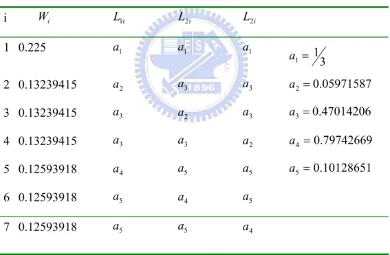
(18) 1 1− L1. ∫∫ f ( x, y) dx dy = ∫ e. 0. ∫ f ( L , L , L ) J(L , L , L ) dL 1. 2. 3. 1. 2. 3. 2. dL1. 0. where |J| is the determinat of the Jacobian matrix and is called Jacobian. The following numerical integration can be applied directly to above integration 7 1 f ( x , y ) dx dy = Wi f ( L1i , L2i , L3i ) J(L1i , L2i , L3i ) ∑ ∫∫e i =1 2 Where subscript i denotes the quantity associated with the sampling point i (i=1 to 7), and the local coordinates, L1i , L2i , L3i are presented in Table 2. 10.

(19) Table 1. Interpolation functions. Edge. {φt }. CT/LN. ⎡φ t 1 ⎤ ⎢φ ⎥ ⎢ t2 ⎥ ⎢⎣φt 3 ⎥⎦. Nodal. i x {U}+ i y {V}. ⎡ J 1 ∇ t L3 1 ( L1∇ t L2 − L2 ∇ t L1 ) ⎤ ⎢ ⎥ ⎢ J 2 ∇ t L1 2 ( L2 ∇ t L3 − L3∇ t L2 )⎥ ⎢ J ∇ t L2 ( L3∇ t L1 − L1∇ t L3 ) ⎥ 3 ⎣ 3 ⎦. Linear. { φz } ⎡φ z 1 ⎤ ⎢φ ⎥ ⎢ z2 ⎥ ⎢⎣φ z 3 ⎥⎦. Table 2. Values of weighting coefficients and local coordinates. Wi. L1i. L2i. L2i. 1 0.225. a1. a1. a1. a1 = 1. 2 0.13239415. a2. a3. a3. a 2 = 0.05971587. 3 0.13239415. a3. a2. a3. a3 = 0.47014206. 4 0.13239415. a3. a3. a2. a4 = 0.79742669. 5 0.12593918. a4. a5. a5. a5 = 0.10128651. 6 0.12593918. a5. a4. a5. 7 0.12593918. a5. a5. a4. i. 11. 3. {N}. ⎡ L1 ⎤ ⎢L ⎥ ⎢ 2⎥ ⎢⎣ L3 ⎥⎦.

(20) Fig. 1. The basis functions of the CT/LN element.. 12.

(21) 1 6 4 2. 5. 3. Point. Local coordinate ( L1 , L2 , L3 ). 1 2 3 4 5. (1,0,0) (0,1,0) (0,0,1) (0.5, 0.5, 0) (0, 0.5, 0.5). 6. (0.5, 0, 0.5) Fig. 2. The local coordinate of a element.. 13.

(22) Chapter 3 The Perfectly Matched Layers 3.1 Introduction to PML The perfectly matched layer (PML) is an artificial medium which serves as an absorbing boundary condition (ABC). This absorbing boundary condition holds great promise for truncating the mesh efficiently in the numerical computation for EM wave problems. It can absorb radiation wave almost without reflection at the absorber interface for arbitrary angle, wavelength and polarization of incidence. In addition, it is also valid for any linear lossy or anisotropic media [F. L. Teixeira, 1998]. Because of the reflectionless, it is termed as “perfectly matched layer,”. The idea of PML was originally proposed by Berenger for FDTD simulation [J. P. Berenger, 1994]. He used the so called “split field,” formalism, in which, for example, Hz is decomposed into Hzx and Hzy. This leads to a modified version of Maxwell equations, where the introduction of the split fields provides extra degrees of freedom that can be used to achieve a perfect reflectionless match at the absorber interface. This is fairly a revolution, since it was quickly shown that the PML outperforms other previous known boundary conditions. In the subsequent years, there are many different interpretations about the physical meaning of PML . Chew et al., indicated that the Berenger’s PML can be derived from a more general way base on the concept of complex coordinate stretching [W. C. Chew et al., 1997], in which the PML can be regarded as a regular isotropic medium but with a complex thickness. Sacks et al., [Z. Sacks, 1995] revealed that the PML also can be considered as an anisotropic medium. In fact, Chew’s and Sacks’ statements are equivalent mathematically [F. L. Teixeira, 1998]. Here, we adopt anisotropic PML in our simulation because in finite element analysis, it is convenient to specify the material parameters (i.e.. 14.

(23) permittivity & permeability) of the PML.. 3.2 The Concept of PML The concept of PML is shown as follow for a plane wave. e -jk0nz One can apply the following coordinate transformation to z z. z → ~z = ∫ s z (z′) dz′ 0. where s z ( z′ ) is so called complex stretched variable [W. C. Chew et al., 1997]. Considering the following structure. z We can let s z (z′) =1 in non-PML region, and s z (z′) = 1- j*c in PML region. In consequence, ~z = z (real) in non-PML region, and ~z = z - j*c*z (complex) in PML region. This implies that the propagation wave would be absorbed in the PML region. Base on this idea, after a series of transformations, the permittivity and permeability tensors in the PML can be expressed as [F. L. Teixeira, 1998]:. ε PML = (det S ) −1[ S ⋅ ε ⋅ S ] µ PML = (det S ) −1[ S ⋅ µ ⋅ S ] Note that the intrinsic impedance of the PML region is equal to that of the. 15.

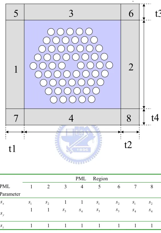
(24) non-PML region, namely, impedance match. So no reflection occurs at the absorber interface. 1 1 1 also S = xˆxˆ ( ) + yˆyˆ ( ) + zˆzˆ ( ) is a diagonal tensor, and sx sy sz (det S ) −1 = s x ⋅ s y ⋅ s z The specification of s x , s y , s z are shown in Fig. 3, where ⎛ρ⎞ s i = 1 - jα i ⎜⎜ ⎟⎟ ⎝ ti ⎠. 2. , i = 1, 2…8.. Here ρ is the distance from the PML interface, and t is the thickness of PML. The attenuation of the field in PML regions can be controlled by choosing the value of α i appropriately.. 16.

(25) 5. 6. 3. 2. 1. 7. 4. sy sz. t4. 8 t2. t1. PML Parameter sx. t3. PML. Region. 1. 2. 3. 4. 5. 6. 7. 8. s1. s2. 1. 1. 1 s3. 1 s4. s1 s3. s2 s3. s1 s4. s2 s4. 1. 1. 1. 1. 1. 1. 1. 1. Fig. 3 The specification of s in the PML.. 17.

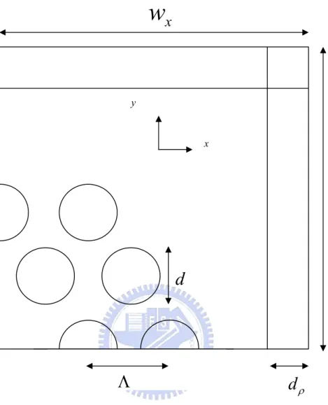
(26) 3.3 Solution Issues In order to reliably predict the features of HFs, the full vector formulation is applied. Because of the losses resulted from the air holes and the finite transverse extent of the confining structure, the effective index is a complex value and its imaginary part is related to the losses. This is termed as a leaky mode. In order to evaluate propagation losses of leaky modes, an anisotropic perfectly matched layer (PML) is employed as an absorption boundary condition at the computational window edges. How to solve the large sparse generalized eigen value problem to get the leaky mode solution is an important issue in finite element procedure. Recently, Koshiba et al., employed the imaginary-distance beam propagation method (ID-BPM) based on the FEM to deal with the leaky-mode problems [K. Saitoh et al., 2002]. On the other hand, Selleri et al., used the Arnoldi method based complex modal solver to obtain several eigen-modes directly [S. Selleri et al., 2001]. The ID-BPM starts the propagation with an initial approximate field and the field evolves into the exact eigen-mode after propagating a long distance. The drawback of this method is that it’s time consuming to achieve high accuracy and only one mode can be obtained each time. On the contrary, solving the eigen-value equation directly is much simpler than the ID-BPM method. For this reason, we use a modified Matlab built-in eigen-solver based on Arnoldi algorithm to treat this problem. The propagation loss of leaky mode is defined as L=. 2 ⋅ 10 7 2π ⋅ ⋅ Im[n eff ] (dB/m) ln(10) λ. Fig. 4 shows the cross section of the HF surrounded by the PML regions with thickness d ρ . Here x and y are the axes of the transverse plane, z is the propagation direction, and Wx and W y are the half computational window. 18.

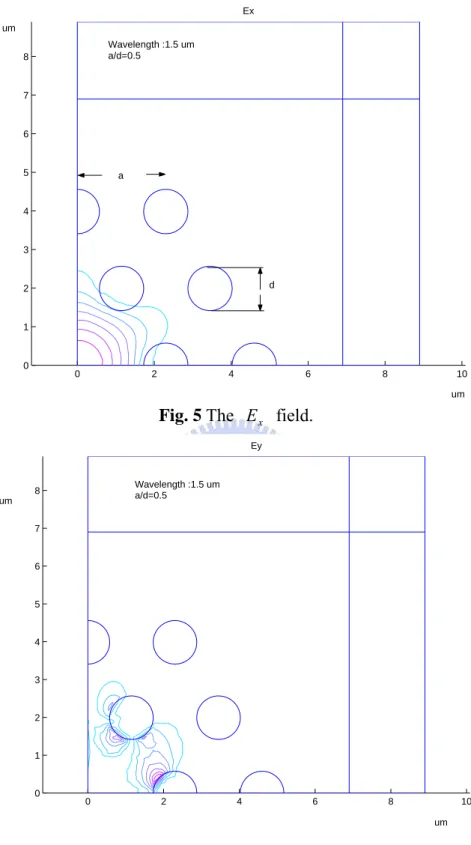
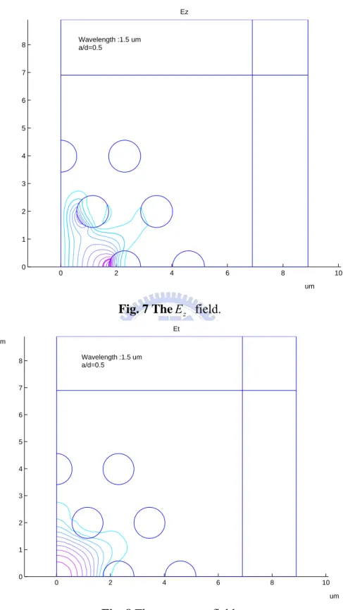
(27) size respectively. The PML parameter S is complex for the leaky mode analysis, which is given as:. S = 1 - jα The parameter s controls the attenuation of the field in the PML region through the choice of the appropriate value of α with the parabolic profile ⎛ ρ α = α max ⎜⎜ ⎝ dp. 2. ⎞ ⎟ ; ⎟ ⎠. where ρ is the distance in the PML region from its inner interface. Consider a PCF with two ring air holes with hexagonal (or triangular ) lattice arrangement, as shown in Fig. 4, the hole pitch Λ =2.3 µm , silica. d = 0.5 , d ρ = 2.3 µm , wx = w y = 7 µm , and Λ operating wavelength λ = 1.5 µm . Because of the six-fold symmetry of this. index = 1.45, air filling ratio. PCF, for the fundamental mode, one-fourth of the fiber cross section combined with proper boundary conditions is taken into computational region. Fig.5 to Fig.8 are the E field distributions for x component, y component, z component and transverse component respectively. Fig.9 and Fig.10 are the effective indices and propagation losses compared with the published results respectively [K. Saitoh et al., 2002].. 19.

(28) wx. y. x. wy. d. Λ. dρ. Fig. 4 The computational window of the PCF.. 20.

(29) Ex um Wavelength :1.5 um a/d=0.5. 8. 7. 6. 5. a. 4. 3. d. 2. 1. 0. 0. 2. 4. 6. 8. 10 um. Fig. 5 The E x field. Ey. Wavelength :1.5 um a/d=0.5. 8 um 7. 6. 5. 4. 3. 2. 1. 0. 0. 2. 4. 6. 8. 10 um. Fig. 6 The E y field.. 21.

(30) Ez. Wavelength :1.5 um a/d=0.5. 8. 7. 6. 5. 4. 3. 2. 1. 0. 0. 2. 4. 6. 8. 10 um. Fig. 7 The E z field. Et um Wavelength :1.5 um a/d=0.5. 8. 7. 6. 5. 4. 3. 2. 1. 0. 0. 2. 4. 6. 8. 10 um. Fig. 8 The transverse field.. 22.

(31) (a). (b) Two-ring air holes 1.45 0.5 0.6. Effective index. 1.44. 1.43. d/a=0.5 d : Hole diameter a : Lattice constant. 1.42. d/a=0.6 1.41. 1.4 0. 0.5. 1 Wavelength um. 1.5. 2. Fig. 9 The effective index of two-ring air holes. (a) Published result in [K. Saitoh et al., 2002]. (b) Our simulation result.. 23.

(32) (a). (b) d B/m. P ro p a g a ti o n L o s s fo r Tw o -ri n g a i r h o l e. 4. 10. 2. 10. d /a =0 .5. 0. L o ss. 10. -2. 10. -4. 10. -6. 10. -8. 10. 0. 0.2. 0.4. 0.6. 0.8. 1. 1.2. 1.4. 1.6. 1.8. Wa ve l e n g th u m. Fig. 10 The propagation loss of two-ring air holes. (a) Published result in [K. Saitoh et al., 2002]. (b) Our simulation result.. 24. 2.

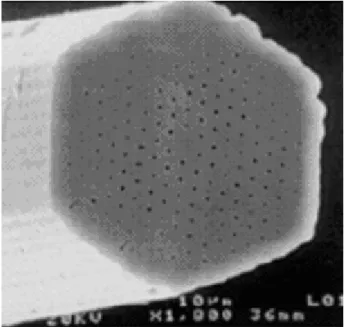
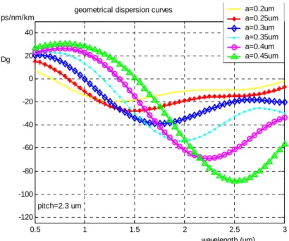
(33) Chapter 4 Optical Properties of PCFs 4.1 Endless Single Mode The picture in fig. 11 shows the structure of a typical holey fiber. In [T. A. Brinks, 1997], the fiber was reported to be single mode over a remarkably wide wavelength range, form 458 to 1550 nm at least, and it is confirmed numerically that HFs are endless single mode for d / Λ <=0.43 [M. Koshiba, 2002]. The cladding effective index, which is a very important design parameter for realizing a single-mode HF, is defined as the effective index of the infinite photonic crystal cladding if the core is absent. Unlike conventional fibers, the effective index of the HF cladding is very sensitive to the wavelength, and has to be estimated for different frequencies by finding the fundamental space filling mode (FSM) of a cladding unit cell, which is shown in Fig. 12. Just like conventional fibers, the effective index of the HF guided mode is between the core index and the effective index of the cladding. Fig. 13 (b) shows our simulation results for the fundamental mode of the PCF, and Fig. 13(a) is the published results with the same structure parameters as in (b). Fig.14 (a) shows the published result of the effective index for the fundamental guided mode and cladding with pitch = 2.3 µm , hole diameter = 0.6 µm . Fig.14 (b) shows the simulation result. The lowest solid line is the cladding effective index, the middle is the fundamental mode effective index, and the user is the core index. We can find that this structure support single mode propagation because only one effective index is found in the region between the core index and the cladding effective index. Fig.15 shows the dispersion curve for different air hole diameters with a fixed pitch of 2.3 µm . One can see that, as the hole diameter increasing, the dispersion zero point shifts to the higher frequency range, and the slope of their linear part is approximately preserved.. 25.

(34) Here, the group velocity dispersion is defined as D=. − λ d2 ⋅ ⋅ Re[n eff ] c dλ 2. 26.

(35) Fig. 11 The endless single mode fiber.. Unit cell for FSM. Fig. 12 Unit cell for FSM estimation.. (a). 27.

(36) (b). Fig. 13 Contour plot of the fundamental mode in the PCF (a) Published results [M. Koshiba, 2002] (b) Our simulation results (a). 28.

(37) (b) core index. Neff. 1.46 1.458 1.456 1.454. neff of guided mode. 1.452 1.45 neff of cladding 1.448 1.446 1.444. pitch=2.3 um. 1.442 1.44. 2. 3. 4. 5. 6. 7. 8. 9. 10. pitch/wavelength. Fig. 14 Effective index of the guided mode of the PCF (a) Published result [M. Koshiba, 2002] (b) Our simulation result. 29.

(38) a=0.2um a=0.25um a=0.3um a=0.35um a=0.4um a=0.45um. geometrical dispersion curves ps/nm/km 40. Dg. 20 0 -20 -40 -60 -80 -100. pitch=2.3 um -120 0.5. 1. 1.5. 2. 2.5 wavelength (um). 3. Fig 15. Our simulation of dispersion curves for a fixed pitch with different air filling ratio a. 30.

(39) 4.2 Mode Classification When higher order modes or polarization properties are considered, the full vector approach is crucial for assessing the true behavior of electromagnetic waves in complex wave-guiding structures such as PCF. It is well known that the PCF is often strongly multimode in the visible and near-infrared regions when the filling factor is large enough. This may lead to a number of intermodally phase-matched nonlinear processes. As a consequence, it is necessary to investigate the modal properties of PCFs including their degeneracy, classification, and so on. Some studies have discussed the mode properties of PCFs [M. J. Steel et al., 2001], and the classification and degeneracy properties of higher-order modes were discussed further in [R. Guobin et al., 2003]. It is shown that the mode classification of a PCF is similar to that of a step-index fiber, except for modes with the same symmetry as the PCF. When the doublet of the degenerate pairs both have the same symmetry as the PCF, they will be split into two non-degenerate modes. In the scalar approximation, the characteristics of polarization in the PCF are hidden. With the full vector aroach, the vector modal behavior of the PCF can be predicted. From the theory of group representations, the symmetry of a waveguide controls several important characteristics of the modes of the waveguide [T. P. White et al., 2002]. Determining the symmetry type of a particular waveguide enables one to classify the possible modes in terms of mode classes, and to predict the mode degeneracies between mode classes. Further, from the azimuthal symmetries of modal electromagnetic fields of a mode class, one can specify a minimum sector of waveguide cross section, together with associated boundary conditions for this sector, which is necessary and sufficient for completely determining all the modes of that mode class. If a uniform wave-guide has n-fold symmetry and also possesses precisely n reflection planes spaced azimuthally by have Cnv. π. radians, it is said to n symmetry. For the triangular lattice PCF, it has six-fold rotation. symmetry and. π 6. reflection symmetry, so the point group is C6v . PCFs. 31.

(40) with the C6 v symmetry possess the following properties: all the modes can be divided into eight classes according to the minimum sector and boundary conditions. As shown in Fig. 16, class p = 1,2,7,8 are non-degenerate, which exhibit full waveguide symmetry, i.e. C6 v symmetry, while class p=3, 4 and p=5, 6 are degenerate pairs, and they exhibit full waveguide symmetry in combination. Table 3 lists the first 14 modes of PCF (with pitch =2.3 um, air filling ratio =0.8, and wavelength = 0.633 um) with effective index, mode class, degeneracy, computation error, and label published in [R. Guobin et al., 2003]. Fig. 17 to Fig. 23 shows the field distribution of these modes. Fig. 24 to Fig. 28 show the fundamental mode and some higher order modes simulated respectively by using the minimum sector with specific boundary conditions belonging to the mode class listed in Table 3. 32.

(41) Fig. 16 Minimum sectors for waveguides with C6 v symmetry, the modes of. waveguides are classified into eight classes (p=1, 2, 3, …8). Solid lines indicate PEC boundary condition, and dashed lines indicate PMC boundary condition [R. Guobin et al., 2003].. Table 3 Mode classes of the triangular-lattice PCF [R. Guobin et al., 2003].. 33.

(42) (a). (b). Fig. 17 HE 11 mode [R. Guobin et al., 2003].. (a). (b). Fig. 18 (a) TE 01 mode (b) HE 21 mode [R. Guobin, 2003].. 34.

(43) (a). (b). Fig. 19 (a) HE 21 mode (b) TM 01 mode [R. Guobin, 2003].. (a). (b). Fig. 20 (a) HE 311 mode (b) EH 11 mode [R. Guobin, 2003].. 35.

(44) (a). (b). Fig. 21 (a) EH 11 mode (b) HE 312 mode [R. Guobin, 2003].. (a). (b). Fig. 22 (a) HE 12 mode (b) HE 12 mode [R. Guobin, 2003].. 36.

(45) (a). (b). Fig. 23 (a) EH 21 mode (b) EH 21 mode [R. Guobin, 2003].. 37.

(46) 2. 1.5. 1. 0.5. 0 −0.5. 0. 0.5. 1. 1.5. Fig. 24 HE 11 mode.. 1.8 1.6 1.4 1.2 1 0.8 0.6 0.4 0.2 0 −0.5. 0. 0.5. Fig. 25 TE 01 mode.. 38. 1. 1.5.

(47) 2 1.8 1.6 1.4 1.2 1 0.8 0.6 0.4 0.2 0 −1. −0.5. 0. 0.5. 1. 1.5. Fig. 26 HE 21 mode.. 2. 1.5. 1. 0.5. 0 −0.5. 0. 0.5. Fig. 27 HE 21 mode.. 39. 1. 1.5.

(48) 2. 1.5. 1. 0.5. 0 −0.5. 0. 0.5. 1. Fig. 28 EH 21 mode. 40. 1.5.

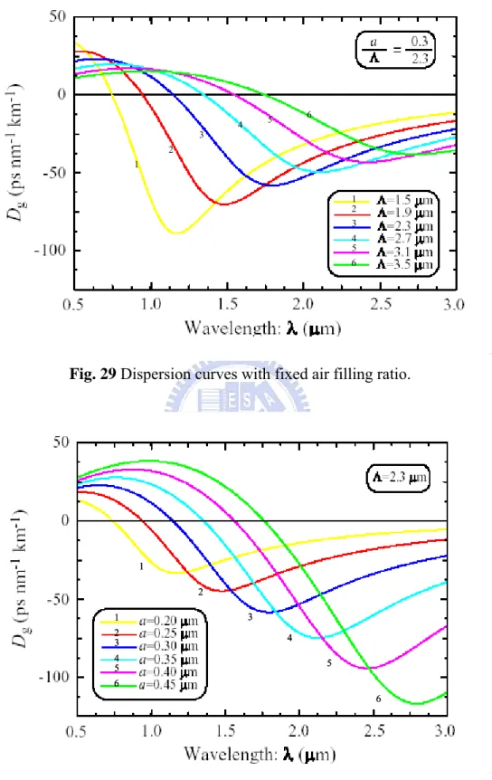
(49) 4.3 Dispersion Flattening Controlling the chromatic dispersion in optical fibers is a very important problem for communication systems. In both linear and nonlinear regimes, or for any optical systems using ultra short soliton-pulse propagation. In all cases, the almost-flattened fiber-dispersion behavior becomes a crucial issue. The most appealing feature of photonic crystal fibers is their high flexibility based on the particular geometry of their refractive index distribution. This fact allows us to manipulate the geometrical parameters of the fiber to generate enormous variety of different configurations. The form of dispersion relation of guided mode for PCFs is very sensitive to the 2D photonic crystal cladding. For this reason, one can expect to control, at least to some extent, the dispersion properties of guided modes by manipulating the geometry of the cladding. It was soon realized that the PCF exhibited dispersion properties very different than those of conventional fibers. As an example, some PCF configurations presenting zero dispersion point bellow that of slica at 1.3 µm [D. Mogilevtsev, 1998; P. J Bennet, 1999], and some others showing flattened dispersion (one point of zero third-order dispersion) or near zero ultra-flattened dispersion (one point of zero fourth-order dispersion) profiles [A. Ferrando et al., 2000]. Since the number of different photonic crystal configurations is significant, one can deduce that it must be possible to elaborate a procedure to tailor the dispersion of the PCF modes in an efficient way. A systematic approach to design the dispersion properties of the PCF using a systematic procedure has been already suggested in [A. Ferrando et al., 2001]. The analogous design details of dispersion flattened or dispersion compensation for triangular lattice PCFs and high-index-core bragg fibers were also proposed in [A. Ferrando et al., 2000], and the dispersion properties of square lattice PCF were discussed recently [A. H. Bouk 2004]. Fig. 29 and Fig. 30 show two sets of PCF geometrical dispersion curves: A. Different pitches with a fixed air filling ratio. B. Different air filling ratios with a fixed pitch. In set A, for different pitches, the dispersion zero point would shift and the slope of each curve in the linear region is different. In set B, for different air. 41.

(50) filling factors, the curves are shifted and the slope of their linear part is approximately preserved. Fig. 31 shows the idea of dispersion flattening design. The line with open circle is the opposite sign of the material dispersion curve, the line with open diamond is the geometrical dispersion curve, and the triangle is the total dispersion, which is defined as D ~= Dg - (-Dm) The key factor to achieve the flattened dispersion curve is the control of the slope of the linear part Dg. The sign changed material dispersion -Dm is a smooth and almost linear curve in most of the infrared region. It is clear from Fig. 31 that if the linear part of geometrical dispersion can be set to be parallel with the material dispersion, therefore the total dispersion will achieve an ideal perfect flattened behavior. The strategy to obtain such a behavior is then straight forward. It can be started by determining the slope of material dispersion curve at some specific wavelength. In the region where the material dispersion curve is smooth, the slope is approximately the same for a reasonably wide neighborhood around the specific wavelength. Once the slope of the Dm is fixed, we can change the pitch and the air hole diameter with a fixed air filling factor to obtain a Dg curve having a linear region with the same given slope of Dm, as shown in Fig. 29. If both the linear part of material and geometrical dispersion curves overlap in a specific wavelength region, then the dispersion flattened curve can be obtained in the overlapping region. After that, we can fix the pitch and change the air hole diameter to get a shifted curve, as shown in Fig. 30. Then different widths of flattened region can be obtained.. 42.

(51) 3. 6. 5. 4. 2 1 1 2 3. 4 5 6. Fig. 29 Dispersion curves with fixed air filling ratio.. 1 2. 3. 1 2 3. 4. 4 5. 5. 6 6. Fig. 30 Dispersion curves with fixed pitch.. 43.

(52) Fig. 31 Schematic mechanism of dispersion flattening design.. 44.

(53) 4.4 Birefringence For conventional polarization-maintaining fibers, the birefringence is made elasto-optically by incorporating different materials close to the core which generate stress when the fiber cools down during the drawing process. The birefringence can also appear due to non-circular core symmetry. High Birefringence fibers serve as polarization-maintaining fibers (PMFs). In standard fiber transmission systems, imperfections in the core-cladding interface introduce random birefringence that leads to light being random polarized. In PMFs, the problems of random birefringence are overcome by deliberately introducing larger uniform birefringence throughout the fiber. Current PMFs, such as bow-tie and panda fibers [K. H. Tsai, 1991], achieve this goal by applying stress to the core region of the standard fiber, creating a modal birefringence up to 5 ⋅ 10 −4 [K. Tajima, 1989]. It is well known that PCFs have more flexibility than conventional fibers in the design of optical fiber properties. According to the recent literature, for PCFs, high birefringence can be produced by the combination of asymmetric core and large core-cladding index contrast [I. K. Hwang, 2004], air holes of two sizes around the fiber core [T. P. Hansen, 2001], and asymmetry obtained by selective filling of air holes with polymer [C. Kergage, 2002]. To-date, the birefringence is reported to be about one order of magnitude lager than conventional fibers, and the largest one is about 3.7 ⋅ 10 -3 [A. O. Blanch, 2000]. In this section, we try to induce high birefringence by incorporating elliptical air hole that has not been proposed in the literature. Two aroaches are considered: A. Different ellipticity (e) with fixed Λ and fixed major axis. B. Different stressing factor for an initially given PCF with pitch Λ and circular air hole diameter d. For case A, as shown in Fig. 32, the ellipticity e (<=1) is defined as the ratio of the minor axis to the major axis, d is defined as hole diameter, and Λ is defined as the pitch or hole-to-hole distance. Table 4 shows the birefringence for e = 0.5 and e= 0.3 with Λ =2.32 µm and major axis. 45. rx =.

(54) 2.088 µm at. λ = 1.5µ m. For case B, another parameter, s (<=1) is. defined as the stressing factor. As illustrated in Fig. 33, for a typical PCF with circular air holes, when a horizontal stress is alied to the PCF, the horizontal dimension of the structure would be scaled by s and the vertical one would be scaled by 1/s. Table 5 shows the birefringence with s = 0.6 and pitch =2.3 µm at. λ = 1.5µ m. Form Table 4 and Table 5, it seems. that class A possesses higher birefringence than class B. But it is still smaller than 10 -3. 46.

(55) h Λ. Λ. d. rx ry Λ. Λ. Fig. 32 Triangular lattice with elliptical air hole with fixed pitch.. 47.

(56) h Λ. Λ. d. h′. Λ′. d′. Fig. 33 Stressed PCF.. 48.

(57) Table 4. Birefringence of class A PCF.. Λ =2.32 µm ,. rx = 2.088 µm , λ = 1.5µ m. E. Neff-x. Neff-y. Birefringence. 0.5. 1.419747033737480 1.419076938826004 6.70 exp(-4). 0.3. 1.425759459962646 1.425236286662941 5.23 exp(-4). Table 5. Birefringence of class B PCF.. S=0.6, Λ =2.32 µm ,. λ = 1.5µ m. D. Neff-x. Neff-y. 2.088. 1.382123939764951 1.382074588315252 4.932 exp(-5). 1.624. 1.404978688533360 1.404917171090318 6.151 exp(-5). 49. Birefringence.

(58) 4.5 Additional Simulation For the first time, we also study the dispersion property of square-lattice PCF with elliptical air holes, which is shown in Fig. 34. The elliptical air holes of this structure are formed by stressing the circular air holes with different stress factor s, which is defined as s=. d′x d. or. d 1 = d ′y s. Here d′x and d′y are the minor axis and the major axis respectively. Another parameter, the air filling ratio a, which stands for the size of the air holes is given as d Λ Fig. 35 shows the dispersion curve for different s with fixed pitch 2.32 µm . a=. In this case, the dispersion slope is positive. Fig.36 shows the dispersion curves with the pitch fixed to 1 µm , and the dispersion slope turns to be negative, thus we can utilize the negative dispersion slope in the dispersion compensation design. Besides, from Fig. 35 and Fig. 36 one can find that the value of dispersion is larger for a large air filling factor a. These two properties are consistent with the case in the square-lattice HF with circular air holes [A. H. Bouk et al., 2004]. What makes difference for this elliptical air holes assisted structure is the vertical dispersion offset. If the air filling ratio a is fixed, the dispersion curve with smaller s moves to higher region. With the stress factor s, designers can have more degrees of freedom to control the dispersion curves in a specific region.. 50.

(59) d. d′y. d′x. Λ. Fig. 34 The square-lattice HF with elliptical air holes.. 51.

(60) Dispersion 95. Ps nm-1 km-1. 90. 85. 80. 75 a=0.7,s=0.8 a=0.7,s=0.9 a=0.6,s=0.8 a=0.6,s=0.9. 70. pitch 2.32 um 65 1.42. 1.44. 1.46. 1.48. 1.5. 1.52. 1.54. 1.56. 1.58. 1.6. um. Fig. 35 Positive GVD (anomalous dispersion) with pitch = 2.32 um. Dispersion -60 a=0.7,s=0.8 a=0.7,s=0.9 a=0.6,s=0.8 a=0.6,s=0.9. -80 -100. Ps nm-1 km-1. -120. pitch 1 um. -140 -160 -180 -200 -220 -240 -260 1.42. 1.44. 1.46. 1.48. 1.5. 1.52. 1.54. 1.56. 1.58. um. Fig. 36 Negative GVD (normal dispersion) with pitch = 1um.. 52. 1.6.

(61) Conclusion and Future Work In this work, a simulation tool for studying the modal properties of optical wave-guides with arbitrary cross-sections has been developed based on the finite element method using CT/LN edge element. In the previous sections, we discuss the optical properties of HFs and demonstrate some simulation results. Finally, for the first time, we discuss the dispersion characteristics of square-lattice HFs with elliptical air holes. It is shown that besides the air filling ratio a, the designer can have one more degree of freedom to control the dispersion curve in a specific region by tuning the stress factor s. For the following days to come, we will continue to work on modifying the code with the use of higher order elements to get fast-converged solutions with fewer unknowns. Moreover, if the optical properties of the wave-guides with longitudinal-variant cross-sections are desired, then the method in this study is not applicable anymore. For this reason, we still need to combine the use of the finite element method with the beam propagation method (BPM) to obtain a complete analysis. Recently, the combination of the finite element and the genetic algorithm (GA) has been demonstrated for obtaining the optimization design of the PCF dispersion property [Emmanuel Kerrinckx, 2004]. We believe that a lot of research efforts still needed in this field. Actually an evolutionary programming algorithm has been developed for the design of fiber gratings in our group. So how to combine the FEM with the optimization algorithm efficiently will be an interesting issue for us to investigate in the future.. 53.

(62) Reference 1.. A. Ferrando et al., “Nearly zero ultraflattened dispersion in photonic crystal fibers,＂Opt. Lett., 790, 2000.. 2.. A. Ferrando et al., “Designing the properties of dispersion-flattened photonic crystal fibers,” Optics Express, Vol.13, 687, 2001 A. H. Bouk et al., “Dispersion properties of square-lattice photonic crystal fibers,＂ Optics Express, Vol.12, 941, 2004. 3. 4. 5.. 6. 7. 8.. A. O. Blanch et al., “ Highly birefringent photonic crystal fibers,” Opt. Lett., vol. 25, 1325, 2000 A. Konrad et al., “Vector variationl formulation of electromagnetic fields in anisotropic media,” IEEE Transactions on Microwave Theory and Techniques, 553, 1976. B. J. Eggleton et al., “Microstructured optical fiber devices,” Optics Express, Vol.9, 698, 2001 C. Kerbage et al., “Highly tunable birefringent microstructured optical fiber,” Opt. Lett , Vol. 27, 842, 2002 D. Mogilevtsev, “Dispersion of photonic crystal fibers,＂ Opt. Lett.,. 1662, 1998. 9. D. Sun et al., “Spurious modes in finite-element methods,” IEEE Antennas and Propagation Magazine, Vol.37, 12, 1995 10. E. Kerrinckx, “Photonic crystal fiber design by means of a genetic algorithm,＂ Opt. Express, vol. 12, 1990, 2004 11. F. Collino et al., “Optimizing the perfectly matched layer,” Computer Methods in Alied Mechanics and Engineering, vol. 164 , 157, 1998 12. F. L. Teixeira et al., “A general approach to extend berenger’s absorbing boundary condition to anisotropic and dispersive media,＂ IEEE Transection on Antennas And Propagation. Vol. 46, 1386, 1998 13. F. L. Teixeira et al., “General closed-form pml consititutive tensors to match arbitrary bianisotropic and dispersive linear media, ＂ IEEE Microwave and Guided Wave Letters, Vol. 8, 223, 1998 14. F. Poli. et al., “Characterization of microstructured optical fibers for wideband dispersion compensation,＂ J. Opt. Soc. Am. A, Vol. 20,. 1958, 2003 15. G. Ouyan et al., “Theoretical studey on dispersion compensation in. 54.

(63) air-core bragg fibers,＂ Optics Express, vol. 9, 899, 2002. 16. G. Ouyang et al., “Comparative study of air-core and coaxial bragg fibers: single-mode transmission and dispersion characteristics, ＂ Optics Express, Vol.9, 733, 2001. 17. I. K. Hwang et al., “Birefringence induced by irregular structure in photonic crystal fiber,＂ Optics Express, Vol.11, 2799, 2003. 18. I. K. Hwang et al., “High birefringence in elliptical hollow optical fiber,＂ Optics Express, Vol.12, 1916, 2004 19. J. C. Knight et al., ＂All-sillica single-mode optical fiber with photonic crystal cladding,＂ Opt. Lett., vol. 21, 1547, 1996 20. J. P. Berenger, “A perfectly matched layer for the absorption of electromagnetic waves,＂ J. Comp. Phys., vol. 114, 185, 1994. 21. J. R. Folkenberg et al., “Polarization maintaining large mode area photonic crystal fiber,＂ Optics Express, Vol.12, 956, 2004 22. J. Mielewski et al., ”Application of the arnoldi method in fem analysis of waveguides,＂ IEEE Microwave and Guided Wave Letters, Vol. 8, 7, 1998 23. J. F. Lee et al., “Full-wave analysis of dielectric waveguides using tangential vector finite elements,＂IEEE Transaction on Microwave 24. 25. 26. 27.. 28.. Theory and Techiniques, Vol.39 , 1262, 1991 J. A. et al., “High-index-core bragg fibers: dispersion preperties,” Optics Express, Vol.11, 1400, 2003 K. P. Hansen et al., “Photonic crystal fibers,”Proceedings SBMO/IEEE MTT-S IMOC , 259, 2003 K. Saitoh et al., “Air-core photonic band-gap fibers: the impact of surface modes,” Optics Express, Vol.12, 394, 2004 K. Saitoh et al., “Chromatic dispersion control in photonic crystal fibers: application to ultra-flattened dispersion,” Optics Express, Vol.11, 843, 2003 K. Tajima, “Ultra low loss and long length photonic cryssstal fiber,＂. Proceedings of OFC 2003, Postdeadline papers, PD1-1, 2003 29. K. Tajima,＂Transmission loss of a 125-um diameter panda fiber with circular stress-alying parts,＂ J. Light Wave Tech., vol. 7, 674, 1989.. 30. K. M. Kaing et al., “Extruded singlemode non-sillica glass holey optical fiber,＂ Electronics Letters, vol. 12, 546, 2002.. 55.

(64) 31. K. H. Tsai, “General solutions for stress-induced polarization in optical fibers,＂ J. Light Wave Tech., vol. 9, 7, 1991 32. K. Saitoh et al., “Full-vectorial imaginary-distance beam propagation method based on a finite element scheme: application to photonic crystal fibers,” IEEE Journal of Quantum Electronics, Vol. 38, 927, 2002 33. K. Saitoh et al., “Leakage loss and group velocity dispersion in air-core photonic bandgap fibers,” Optics Express, Vol. 11, 3100, 2003 34. K. Saitoh et al., “Photonic bandgap fibers with high birefringence,” IEEE Photonics Technology Letters, Vol. 14 , 1291 ,2002 35. L. S. Anderson et al., “Mixed-order tangential vector finite elements for triangular elements,” IEEE Antennas and Propagation Magazine, Vol. 40, 104, 1998 36. J. F. Lee et al., “High performace electro-optic polymer waveguide device,” Al. Phys. Lett., vol. 71, 3779,1997 37. J. F. Lee, “Finite element method with curvilinear hybrid edge/nodal triangular-shaped elements for optical waveguide problems,＂ M.S. Thesis, Institute of Communication Engineering, National Taiwan University, Taiwan, 2002 38. M. Hano, “Finite-element analysis of dielectric-loaded waveguides,＂. 39. 40. 41. 42.. 43.. 44.. IEEE Transactions on Microwave Theory and Techniques, MTT-32, 1275, 1984. M. Hara, “Three dimensional analysis of rf electromagnetic field by the finite element method,” IEEE Transactions on Magnetics, 2417, 1983. M. J. Steel et al., “Elliptical-hole photonic crystal fibers,” Optical Society of America, Vol. 26, 229, 2001 M. Koshiba et al., “Structural dependence of effective area and mode field diameter for holey fibers,” Optics Express, Vol. 11, 1746, 2003 M. Koshiba et al., “A vector finite element method with the high-order mixed-interpolation-type triangular elements for optical waveguiding problems,” Journal of Lightwave Technology, vol. 12, 495, 1994 M. Koshiba et al., “Curvilinear hybrid edge/nodal elements with triangular shape for guided-wave problems,” Journal of Lightwave Technology, vol. 18, 737, 2000 M. Koshiba et al., “Finite-element analysis of birefringence and. 56.

(65) 45.. 46.. 47. 48. 49. 50. 51.. dispersion properties in actual and idealized holey-fiber structures,” Applied Optics, Vol. 42, 6267, 2003 M. Koshiba et al., “Numerical verification of degeneracy in hexagonal photonic crystal fibers,” IEEE Photonics Technology Letters, Vol. 13, 1313 ,2001 M. Koshiba et al., “Simple and efficient finite-element analysis of microwave and optical waveguide,” IEEE Transaction on Microwave Theory and Techniques, Vol. 40 , 371, 1992 M. Koshiba. “Full-vector analysis of photonic crystal fibers using the finite element method,” IEICE Trans. Electron., Vol.E85-C, 881, 2002 P. J. Bennet, “Toward practical holey fiber technology: fabrication,” Opt. Lett, 1203, 1999. P. Szarniak et al., “Modeling of highly birefringent photonic fiber with rectangular air holes in square lattice,” ICTON, 216, 2003 R. Guobin et al., ,”Mode classification and degeneracy in photonic crystal fibers,” Optics Express, Vol. 11, 1310, 2003 S. G. Johnson et al, “Breaking the glass ceiling: hollow omniguide fibers,＂ Optics Express, vol. 10, 899, 2002.. 52. S. Selleri et al., “Complex fem modal solver of optical waveguides with pml boundary conditions,” Optical and Quantum Electronics, Vol. 33, 359, 2001 53. T. A. Brinks et al., “Endlessly single-mode photonic crystal fiber,” Optical Society of America, Vol. 22, 961,1997 54. T. P. White et al., “Multiple method for microstructured optical fibers. I. Formulation,” J .Optical Society of America B, Vol. 19, 2322, 2002 55. T. Fujisawa et al., “Finite element characterization of chromatic dispersion in nonlinear holey fibers,” Optics Express, Vol. 11, 1481, 2003 56. T. M. Monro et al., “Holey optical fibers: an efficient modal model,” Journal of Lightwave Technology, vol.17, 1093, 1999 57. T. P. Hanson et al., “Highly birefringent index-guiding photonic crystal fibers,” IEEE Photonics Technology Letters, Vol.13 , 588 , 2001 58. W. C. Chew et al., “complex coordinate stretching as a generalized absorbing boundary condition,＂ Microwave Opt. Technol. Lett., 363, 1997.. 57.

(66) 59. W. Zhi et al., “Compact supercell method based on opposite parity for Bragg fibers,” Optics Express, Vol. 11, 3542, 2003 60. X. Xu et al., “Arbritarily oriented perfectly matched layer in the frequency domain,” IEEE Transaction on Microwave Theory and Techniques, Vol. 48 , 461, 2000 61. Y. Tsuji et al., “Guided-mode and leaky-mode analysis by imaginary distance beam propagation method based on finite element scheme,” Journal of Lightwave Technology, Vol. 18, 618, 2000 62. Z. Sacks, “A perfectly matched anisotropic absorber for use as an absorbing boundary condition, ＂ IEEE Trans. Atennas Propagat., 1460, 1995. 58.

(67)