國立交通大學
電機與控制工程學系
碩士論文
以時域和頻域的方法來探討禪坐心電圖的特性
Meditation ECG Characterization by Time- and
Frequency-Domain Methods
研 究 生: 李啟弘
指導教授: 羅佩禎 教授
以時域和頻域的方法來探討禪坐心電圖的特性
Meditation ECG Characterization by Time- and
Frequency-Domain Methods
研 究 生: 李啟弘 Student : Chi-hung Lee
指導教授: 羅佩禎 博士 Advisor : Dr. Pei-Chen Lo
國 立 交 通 大 學 電 機 與 控 制 工 程 學 系
碩 士 論 文
A Thesis
Submitted to Department of Electrical and Control Engineering
College of Electrical Engineering and Computer Science
National Chiao Tung University
In Partial Fulfillment of the Requirements
For the Degree of Master
In
Electrical and Control Engineering
January 2005
以時域和頻域的方法來探討禪坐心電圖的特性
研究生: 李啟弘 指導教授: 羅佩禎
國立交通大學電機與控制工程學系碩士班
摘 要
本研究的目的在於探討禪坐時心電圖的變化,結果將與靜坐休息下的控制組 作比較。心率變異特性分析對評估心臟自主神經的調節功能已被證實是有效且是 非侵入式的分析工具,所以我們可以藉由心率變異特性來評估禪定對心臟自主神 經調節功能的影響。本研究總共收集了 43 位受測者的實驗資料(實驗組:25 人; 控制組:18 人),我們的目的是要分析兩組間統計上的差異。分析方法為時域分 析和頻域分析,而其結果是根據一些要素如受測者的性別和坐姿來加以分析,最 後量化的特徵將依時域和頻域分析中的各個參數以 FCM(Fuzzy C-means)來作分 類。 由實驗結果得到兩個結論:(1) 在時域分析方面,實驗組中採雙盤坐姿的受 測者平均來說,在禪定過程當中所有的參數值(MRR,SDRR,RMSSD)都是減少的,而 控制組平均而言,參數 SDRR 和 RMSSD 在休息過程中是呈現增加的趨勢;(2) 在 頻域分析方面,代表交感神經活性的參數 nLF 和代表自律神經系統平衡的參數 Ratio of LF/HF,實驗組中採單盤坐姿的受測者平均來說,是低於控制組的;相 反的,代表副交感神經活性的參數 nHF、HF,實驗組中採單盤坐姿的受測者平均 來說,則是高於控制組的。 因此可以推測禪定與放鬆休息對心率變異和自主神經系統的調節有不同的 效果.而不同的禪定姿勢所造成的效果亦不相同。Meditation ECG Characterization by Time- and
Frequency-Domain Methods
Student: Chi-hung Lee Advisor: Pei-chen Lo
Institute of Electrical and Control Engineering
National Chiao Tung University
Abstract
The purpose of this research is to discuss the variation of ECG during meditation, and the result will be compared with that of the control group under resting. The analysis of heart rate variability is verified to be effective for estimating the modulation of heart autonomic nerves, and it is also a non-invasive analyzing tool. So we may make use of HRV (heart rate variability) to evaluate the effect of meditation on the modulation of heart autonomic nerves. There are 43 subjects (experimental subjects: 25; control subjects: 18) in this research totally. We aim to analyze the statistical difference between two groups. The analyzing methods include time domain analysis and frequency domain analysis. The results are analyzed according to such factors as gender and meditation posture of the subjects. Finally quantitative features are classified by FCM ( Fuzzy C-means ) depending on each parameter in time and frequency domain analysis.
Two conclusions are drawn from the results:(1) In the time-domain analysis, all the parameters (MRR, SDRR, and RMSSD) tend to decrease when the experimental subjects adopting full-lotus posture enter the meditation session. In the control group, SDRR and RMSSD increase during the resting process. (2) In the frequency-domain analysis, the parameter reflecting the activation of sympathetic system, nLF, and the parameter indicating the balance of autonomic nervous system(ANS), ratio of LF/HF, are both higher for the control subjects in comparison with those of the experimental subjects who adopt half-lotus posture. On the contrary, the parameters reflecting the activation of parasympathetic system, nHF, and HF of the control subjects are lower than those of the experimental subjects who adopt half-lotus posture.
Therefore we may infer that the effects of meditation on the HRV and on the modulation of ANS are different from those of resting. In addition, the results obtained from meditators using various meditation postures are also distinct.
誌 謝
本篇論文的完成,首先要感謝我的指導教授羅佩禎老師,因為她適時的指 導讓我在專業知識的獲取和研究學問的方法上都獲益良多。同時,也要感謝邱 俊誠教授和楊谷洋教授對本論文提出許多建設性的指導與建議。 在碩士班兩年多的學習過程中,我要感謝剛鳴、瑄詠、憲政、權毅、適達 以及清泉幾位博士班學長姐經常給我指導、建議與鼓勵。特別是剛鳴學長一年 多來,對本論文的不吝賜教,使得本論文得以更加完整。而實驗室的同學岳昌 和清文,也感謝你們和我一起努力。另外要感謝學弟偉源、富滄、進忠和偉凱, 在我研究之餘陪我一起度過。 最後,我要感謝我的 師父與我的父母,謝謝你們對我的指引與支持,還 有許多同修和家人對我的關心和照顧,讓我在完成學業的過程中,收穫滿行囊。Contents
1 Introduction 1
1.1 Background and Motivation . . . 1
1.2 Domestic and Overseas Research . . . 2
1.3 Scope of This Research Study . . . .. . . 6
2 Background of Physiological Signal Systems 7
2.1 Introduction to Electrocardiogram . . . 7
2.2 Autonomic Nervous System and Cardiovascular System Modulation . . . 12
2.3 Physiological Indexes Affecting Cardiac Output . . . .. . . 14
2.4 Analysis of Heart Rate Variability . . . .. . . 15
2.4.1 History of heart rate variability . . . .. . 15
2.4.2 Methods of analyzing heart rate variability . . . 16
2.4.3 Characteristics of power spectrum of heart rate variability . . . 18
3 Theoretical Model and Methods……… 20
3.1 Physiological signal collecting system . . . 21
3.2 QRS detection in ECG and heart rate calculating. . . 23
3.2.1 Tompkins QRS detection algorithm . . . .. . . 24
3.2.2 Eliminating ectopic beats. . . 28
3.2.3 Heart rate calculating. . . 30
3.3 Analysis of Poincare scattering plot . . . 36
3.4 Pattern Recognition based on Fuzzy c-Means Algorithm . . . 43
4 Statistical meaning and clustering of ECG 45
4.1 The analysis of ECG in time domain . . . 46
4.1.1 Statistical analysis . . . 46
4.1.2 Analysis with Fuzzy C-Means Clustering . . . 59
4.2 The analysis of ECG in frequency domain. . . .. . . 63
4.2.1 Statistical analysis . . . 63
4.2.2 Analysis with Fuzzy C-Means Clustering . . . 81
5 Conclusion and Discussion 89
5.1 Summary of the current Work. . . 89
5.2 Future Work . . . .. . . 97
List of Tables
3.1 Time domain parameters of HRV . . . 33 3.2 Frequency domain parameters of HRV. . . .35 4.1 Label of identification and number of subjects in each group . . . .49 4.2 (Value in the parentheses) means the subtraction of the parameter in Section4
from that in Section5 . . . .55 4.3 P-value . . . .56 4.4 Parameter (male) Section I – parameter (female) Section I based on the same posture
in 5 sections (M: male; F: female) . . . .56 4.5 Tendency from Section 2 to Section 4 (during meditation course or resting
course) . . . 57 4.6 The classified results of the differences of the 3 parameters from Section 2 to
Section 4; the number of subjects (of a group) being classified to a particular
cluster. . . 60 4.7 The classified results of the differences of the 3 parameters from Section 4 to
Section 5; the number of subjects (of a group) being classified to a particular
cluster. . . 62 4.8 P-value . . . .75 4.9 Parameter (male) Section I – parameter (female) Section I based on the same posture
4.10 Difference between the mean of each parameter of each group and that of all groups in Section 1. . . .77 4.11 Difference between the mean of each parameter of each group and that of all
groups in Section 2. . . .77 4.12 Difference between the mean of each parameter of each group and that of all
groups in Section 3. . . .78 4.13 Difference between the mean of each parameter of each group and that of all
groups in Section 4. . . .78 4.14 Difference between the mean of each parameter of each group and that of all
groups in Section 5. . . .79 4.15 The mean value of the differences in 5 sections (‘difference’ means the
difference between the mean of each parameter of each group and that of all groups in one of the 5 sections) . . . 79 4.16 The classified results of nLF vs. nHF in Section 1; the number of subjects (of a
group) being classified to a particular cluster. . . 82 4.17 The classified results of nLF vs. nHF in Section 2; the number of subjects (of a
group) being classified to a particular cluster. . . 83 4.18 The classified results of nLF vs. nHF in Section 3; the number of subjects (of a
group) being classified to a particular cluster. . . 85 4.19 The classified results of nLF vs. nHF in Section 4; the number of subjects (of a
group) being classified to a particular cluster. . . 86 4.20 The classified results of nLF vs. nHF in Section 5; the number of subjects (of a
group) being classified to a particular cluster. . . 87 5.1 P-value . . . .89 5.2 Parameter (male) Section I – parameter (female) Section I based on the same posture
5.3 Tendency from Section 2 to Section 5 (from the beginning of the meditation to the post test) . . . .91 5.4 The mean value of the differences in 5 sections (‘difference’ means the difference
between the mean of each parameter of each group and that of all groups in one of the 5 sections) . . . 94
List of Figures
2.1 The conduction system of Heart . . . 8
2.2 (A) Bipolar Standard leads (B) Augmented Unipolar leads. . . .9
2.2 (C) Unipolar Chest leads. . . .10
2.3 The standard wave patterns of ECG . . . .11
2.4 Physiological modulating factors of cardiac output . . . .14
2.5 (a) Power spectrum of HRV with 3 major peaks (b) Power spectrum of HRV under parasympathetic blockade and combined parasympathetic and sympathetic blockade . . . . .. . . 19
3.1 The processing procedure for ECG signal . . . .20
3.2 The physiological signal collecting system . . . .21
3.3 Bipolar limb lead I. . . 22
3.4 Standard Electrocardiograph. . . .23
3.5 Flow chart of HRV analysis. . . 23
3.6 Tompkins QRS detection algorithm. . . 24
3.7 Flow chart of R wave detection algorithm (a) Original signal (b) Output of band-pass filter (c) Output of differentiator (d) Output after squaring (e) Result after moving window-integration. . . .25
3.8 (a) ECG signal with baseline wandering and high frequency noise interference (b) The same ECG signal after bandpass filter. . . .26
3.9 Result of R wave Detection . . . .28
3.10 (a) premature atria contraction (PAC) (b) premature ventricular contraction (PVC) . . . . .. . . 29
3.11 (a) Abnormal ECG signal (b) Modification of ectopic heartbeat . . . .30
3.12 HRV signal. . . 30
3.13 Heart rate signal after equal sampling (a) a section of RR intervals (b) heart rate signal after equal sampling when the center point of the local window falling at t1, n = a/ Ii 2, at t2 n = b/Ii 3+c/I4. . . 32
3.14 Result after equal sampling (﹡is the point after re-sampling) . . . 32
3.15 Power spectrum of HRV. . . 34
3.16 The drawing of Poincare scattering plot. . . .36
3.17 Comet shape. . . 38
3.18 Torpedo shape . . . 38
3.19 Fan shape. . . 39
3.20 Complex shape. . . 39
3.21 Long-axis length (SD1) and short-axis length (SD2) of the Poincare plot . . . 40
4.1 Experimental procedure. . . 47
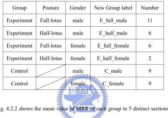
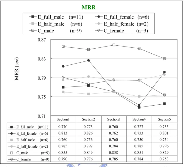
4.2.1 Mean value of MRR (mean value of RR intervals for 5 minutes) of each group in five distinct sections (solid circle E: Experimental group; open circle C: Control group) . . . 48
4.2.2 Mean value of MRR (mean value of RR intervals) of each group in five distinct sections . . . .50
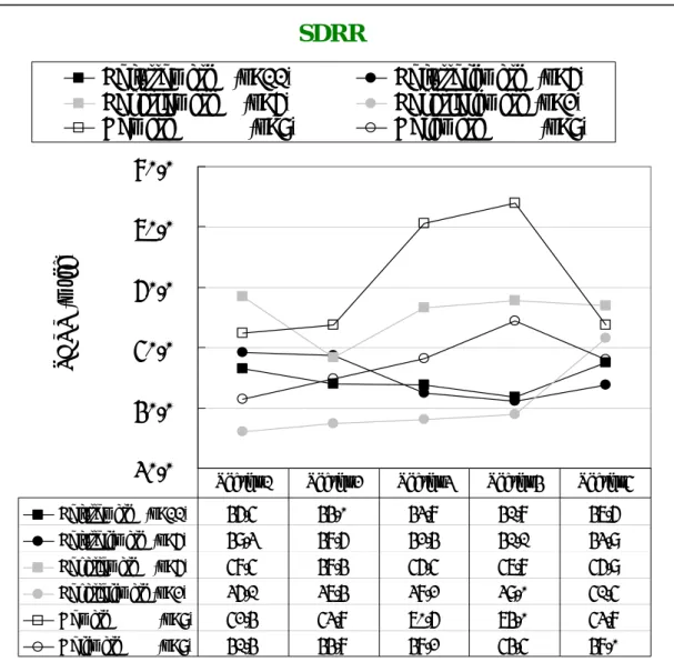
4.3.1 Mean value of SDRR (standard deviation of RR intervals) of each group in five distinct sections (solid circle E: Experimental group; open circle C: Control group) . . . 51
4.3.2 Mean value of SDRR (standard deviation of RR intervals) of each group in five distinct sections . . . .52 4.4.1 Mean value of RMSSD ( root mean square value of the difference of all the
successive RR intervals ) of each group in five distinct sections (solid circle E: Experimental group; open circle C: Control group) . . . .53 4.4.2 Mean value of RMSSD (root mean square value of the difference of all the
successive RR intervals) of each group in five distinct sections . . . 54 4.5 The classified results of the differences of the 3 parameters from Section 2 to
Section 4 using Fuzzy C-means algorithm. . . .60 4.6 The classified results of the differences of the 3 parameters from Section 4 to
Section 5 using Fuzzy C-means algorithm. . . .62 4.7.1 Mean value of pLF (low-frequency power) of each group in five sections (solid
circle E: Experimental group; open circle C: Control group) . . . 64 4.7.2 Mean value of pLF (low-frequency power) of each group in five distinct
sections. . . 65 4.8.1 Mean value of pHF (high-frequency power) of each group in five sections (solid
circle E: Experimental group; open circle C: Control group) . . . 66 4.8.2 Mean value of pHF (high-frequency power) of each group in five distinct
sections. . . 67 4.9.1 Mean value of nLF (normalized low-frequency power) of each group in 5
sections (solid circle E: Experimental group; open circle C: Control group) . . . 68 4.9.2 Mean value of nLF (normalized low-frequency power) of each group in five
distinct sections . . . .69 4.10.1 Mean value of nHF (normalized high-frequency power) of each group in 5
4.10.2 Mean value of nHF (normalized high-frequency power) of each group in five distinct sections. . . .71 4.11.1 Mean value of the ratio of LF/HF for each group in five sections (solid circle E:
Experimental group; open circle C: Control group) . . . 72 4.11.2 Mean value of the ratio of LF/HF for each group in five distinct sections. . . . .74 4.12 The classified result of nLF vs. nHF in Section 1 using Fuzzy C-means
algorithm. . . .82 4.13 The classified results of nLF vs. nHF in Section 2using Fuzzy C-means
algorithm. . . 84 4.14 The classified results of nLF vs. nHF in Section 3 using Fuzzy C-means
algorithm. . . 85 4.15 The classified results of nLF vs. nHF in Section 4 using Fuzzy C-means
algorithm. . . 86 4.16 The classified results of nLF vs. nHF in Section 5 using Fuzzy C-means
algorithm. . . 88 5.1 (a)(b) Difference of MRR, SDRR, and RMSSD from Section 2 to Section 4 (c)(d)
Difference of MRR, SDRR, and RMSSD from Section 4 to Section 5. . . .93 5.2 (a) nLF vs. nHF in Section 1 (b) nLF vs. nHF in Section 2
(c) nLF vs. nHF in Section 3 (d) nLF vs. nHF in Section 4
Chapter 1
Introduction
1.1 Background and Motivation
There are now considerable clinical evidences and a number of theories describing meditation’s impact on psychological and physiological symptoms. Ramita Bonadonna mentioned that meditation practice could positively influence the experience of chronic illness and could serve as a primary, secondary and tertiary prevention strategy [33]. Vernon A. Barnes discovered that Transcendental Meditation program appeared to have a beneficial impact on cardiovascular functioning at rest and during acute laboratory stress in adolescents at-risk for hypertension [38]. Linda E. Carlson proved that Mindfulness-Based Stress Reduction meditation program enrollment was associated with enhanced quality of life and decreased stress symptoms in breast and prostate cancer patients [16]. Elizabeth Monk-Turner found that the subjects practicing meditation benefited most in the aspect of experiencing fewer symptoms of aching muscles or joints that resulted in less use of drugs and tranquilizers [7]. Laurie Keefer demonstrated that constant practice meditation was particularly effective in reducing the symptoms of abdominal pain and flatulence ; Relaxation response meditation is a beneficial treatment for irritable bowel syndrome in both the short-term and the long-term cases [17,18]. John Ding-E Young and Eugene Taylor denoted that there were many physiological analogies between the long-term meditators and hibernators on the phylogenetic scale [13]. Gregory A. Tooley revealed that meditation could affect plasma melatonin levels either by decreasing hepatic metabolism of the hormone or
via a direct effect on pineal physiology. Facilitation of higher physiological melatonin levels at proper times of day might be one way of health promoting effects of meditation [8]. John J. Miller showed that an intensive but time-limited group stress reduction intervention based on mindfulness meditation could have long term beneficial effects in the treatment of people diagnosed with anxiety disorders [14].
The advantage of meditation has drawn our attention. Our research group has been focusing on meditation EEG analysis for several years. We have a great achievement in the development of EEG analysis and interpretation algorithms. And the methods and technologies supporting our research work are getting matured. In recent years, we began extending our research field to other physical signals such as ECG (electrocardiograph), GSR (galvanic skin response), etc. In ECG study, Renlong Tsai used several methods including time domain analysis, frequency domain analysis, time-frequency domain analysis and poincare plot to examine the characteristics of HRV (heart rate variability) of the experimental and control groups. Furthermore, he discussed the correlation between the HRV parameters and ANS (autonomic nervous system). Since he only analyzed few subjects, we need to get a statistically meaningful conclusion by analyzing a larger amount of samples. Thus, in this research we sample more subjects from each group in order to identify the difference of the HRV characteristics between two groups.
1.2 Domestic and International Research Overview
In 1981 Akselrod [34] found that the HRV spectrum was able to tell the difference from the sympathetic effect to the parasympathetic one. Numerous signal-processing methods were adopted to analyze the correlation between HRV
and ANS. And ANS was evaluated for quantifying the variation of heart rate modulation under different kinds of diseases. In other words, results of the spectrum analysis of HRV might provide a tool to explore the ANS without invasion. Therefore HRV has become the dominant agent in the research of autonomic nervous system function. Several kinds of clinical applications of HRV are described separately:
I. Cardiovascular disease
HRV is a powerful index of prognosis for the patient of acute myocardial infarction. SDRR (standard deviation of RR intervals), LF (low frequency power) may be the prognosis index of mortality for the patient with heart exhaustion. When one’s SDRR falls down, his mortality rises up [27]. The clinical reason is that the sympathetic dominates and the modulation effect of sinoatrial node vagi is getting weaker. The decreasing degree of time domain index of HRV is related to how serious the disease is. The correlation between the frequency index of HRV and the disease is more complicated. When one has minor heart failure, his LF increases obviously and HF (high frequency power) decreases. When one has serious heart exhaustion, both his LF and HF power reduce gradually and the rest power distributes in VLF (very low frequency power) band [28,19].
II. Hypertension
In the heart research project, Framingham found that LF corresponded obviously to the hypertension in all of the indexes such as SDRR, LF, HF, LF/HF ratio, and so forth for the HRV estimation of the hypertensive. It is more likely for the one with low LF to become a hypertensive patient [35].
III. Cerebral blood vessel disease
The patient of Parkinson's disease has lower values of SDRR, LF and HF than the healthy subjects of control group at night [23]. In the research of acute head injury in children, when the cerebral perfusion pressure is smaller than 40 mmHg, LF/HF ratio may decrease rapidly [1].
IV. Brain death
For the patient with brain death, the spectrum of LF is becoming zero; otherwise, the spectrum of HF is still quite weak, and LF/HF ratio may drop down [2].
V. Diabetes mellitus
In the experiment, Ewing confirmed that LF and HF were apparently less for the patient with pathological changes of autonomic nervous system. Thus HRV can be a tool of evaluating pathological changes of ANS for diabetics [42]. Pathological changes of ANS for diabetics usually exhibit some conditions: (1) mostly, all power spectrums reduce; (2) when one stands without raising his LF, it indicates the abnormality of the sympathetic reflection; (3) total power reduces exceptionally and LF/HF ratio keeps constant; and (4) when LF tends towards left, its physiological meaning needs to be evaluated further [28].
VI. Gynecologic disease
LF is higher and HF is lower in corpus luteum period than those in follicle period. The activation of sympathetic is higher in corpus luteum period than that in follicle period [36].
Some independent variables affecting HRV are described as follows : I. Gender
The LF of female is lower than that of male, and HF/LF ratio is higher for women [20]. There are no significant differences between men and women for older people. For younger people, men have lower heart rates than women. And all 24-hour time domain indexes of HRV, except those that reflect vagal modulation of heart rate, are significantly higher than those in women [37].
II. Age
With aging, power spectrum relating to the phenomena of sympathetic and parasympathetic diminishes [20,37]. HF/LF ratio is similar between aged people and the young [20].
III. Sport
Experienced athletes exhibit higher modulation effect of parasympathetic and they have better ANS function than the control group. SDRR, LF, HF, and total power are higher in veteran sportsmen, while LF/HF ratio is lower in this group [43].
IV. Alternating between Day and Night
For children, LF/HF ratio is higher during the day than at night. Other HRV indexes such as SDRR, VLF, LF, RMSSD, and HF increase by night and decrease by day [24]. For adult, heart rate, LF/HF ratio, and LF increase during the day; and HF and RR interval increase at night [26].
V. Sleep
For young men, sleeping from awake state to non-REM (rapid eye movement) state, their R-R intervals increase and HF power rises [6]. For the normal, LF/HF ratio reduces obviously from awake state to non-REM state, whereas it rises in REM
LF/HF ratio increases obviously from awake state to non-REM state, and it rises further in REM state. Myocardial infarction causes the disability of the vagal activity. It explains why sudden death attacks myocardial infarction patients at night [39].
VI. Occupation
HF is lower for the high consumption of physical strength and the difference of LF/HF ratio is unclear. The function of ANS may decay gradually in the laborers who burn the candle at both ends [40].
VII. Pregnancy and Menopause
LF is lower in a mother-to-be than in a normal woman. HF is lower and LF/HF ratio rises up for the women during menopause. It indicates that the control function of ANS is disordered. Hormone substitute therapy may improve excessive sympathetic activation [29].
1.3 Scope of This Research Study
This thesis is composed of five parts. Chapter 1 is to describe the research background and motivation, introduce domestic and international researches, and illustrate the organization of this thesis. In Chapter 2, the basic principles of ECG and the relationship between autonomic nervous system and cardiovascular system will be presented. The QRS detection algorithm, the methods for analyzing HRV in time and frequency domain, and the clustering method are illustrated in Chapter 3. Chapter 4 discusses the statistical meaning and clustering results of the ECG features between the experimental and control groups. Chapter 5 summaries this research work and brings forth further research topics to be conducted in the future.
Chapter 2
Background of Physiological Signal Systems
Many physiological signals of human being can be detected and transformed to electric signals. Then we can do some works such as recording, displaying, and analyzing with the help of clinical electronic meter. These signals can aid to the diagnosis of the cause of disease by proper interpretation. Therefore, physiological signals are very valuable in clinical reference. Among all the physiological signals, noninvasive measurements are carried out most often in hospitals, which include ECG, EMG(electromyograph), EEG(electroencephalograph), blood pressure, temperature, etc. Because this research is to analyze the characteristics of HRV (heart rate variability), we put emphasis on the process and analysis of cardiac-electric signals. We thus will go a step further to discuss the features and mechanism of cardiac-electric signals. Biological and physiological background will be illustrated in this chapter. First, principles of ECG, and definitions of ECG profile are introduced. Next, the relation between ANS (autonomic nervous system) and cardiovascular system and their mutual interaction are explained. Then the physiological indexes affecting cardiac output (CO) are listed. Finally, the correlation between HRV and ANS will be depicted.
2.1 Introduction to Electrocardiogram
In the early embryo period, a heart can throb although it just formed and it cannot stop pulsing at any moment until a person die. Heart itself owns the feature of
specialized conducting system inclusive of four parts, that is, SA node (sino-atrial node), AV node (atrio-ventricular node), Bundle of His, and Purkinje fibers. Figure 2.1 shows the anatomic description.
SA node is the pacemaker of heart. It controls the regular pulse of heart entirely. Depolarization waves originate in it, like pebbles falling into a pool. They spread around tier by tier. Depolarization waves propagate to atria (right first and left last), causing atria systole, and “P” wave appears in ECG. Besides, they also spread to AV node. AV node connects with Bundle of His, and Purkinje fibers are the extended part of the fibers of Bundle of His. Purkinje fibers are distributed such as a threadlike net on subenocardial surface. Thus the depolarization waves caused by the pacemaker propagate to atria all around and induce the two atria to draw back. Then they pass to AV node, spread to ventricles widely, and make two ventricles contract simultaneously. Therefore, the order of heart excitation is: SA node → myocardium (atria) → AV node → Bundle of His → Purkinje fibers → myocardium (ventricle) [44].
When heart beats, the depolarization waves resulting from myocardium not only extend to the whole heart, but also make electrical current change. This current will spread to the surface of body so that we may record it with electrocardiograph. The graph we get is called the ECG (electrocardiogram). In general, there are two ways to record ECG; one is bipolar lead and the other is unipolar lead.The method of bipolar recording is to attach the recording electrodes to two hands and two legs, and select right-leg electrode as a reference. Lead I is the voltage difference between left hand and right hand. Lead II is the voltage difference between right hand and left leg. Lead III is the voltage difference between left leg and left hand. (Figure 2.2A) The method of unipolar recording is to connect left hand with left leg to a joint. The voltage between the joint and the right hand is measured. The other way is to connect right hand and left leg to a joint. The voltage between the joint and the left hand is compared. This way is usually called augmented unipolar limb lead, and right leg is still the reference. (Figure 2.2B) Another method of unipolar is to attach six electrodes to the special locations on chest. The voltages measured by the six electrodes at adjoining locations are V1, V2, V3, V4, V5, and V6. (Figure 2.2C)
Fig 2.2 (C) Unipolar Chest leads [45]
Due to the negative potential in the quiescent state (-80mv or so), or so-called polarization, once heart cells are stimulated electrically, and become depolarized, they bear positive potential that activation potential induces the systole reaction. At the same time, ECG traces the potential variation of periodic activity of the heart. The standard wave patterns of ECG are shown in Figure 2.3. The physiological meaning of each normal electrocardiographic complex is described below:
P wave: This deflection is due to the atria depolarization
Q wave: This first negative deflection is caused by the ventricle depolarization. The first positive deflection (R) follows.
R wave: This first positive deflection caused by the ventricle depolarization.
S wave: This first negative deflection follows the first positive deflection (R) during the period of ventricle depolarization.
T wave: This deflection is due to the ventricle repolarization.
U wave: The deflection succeeds the T wave and leads the next P wave. (A positive wave in usual) The mechanism generating this wave forms is unclear yet. One proposal referred this phenomenon to the slower repolarization of the conducting system among ventricles (Purkinje fibers).
The characteristic interval values are introduced briefly as follows:
RR interval: RR interval stands for the time interval between two successive R waves. The BPM (beat per minute) can be derived by 60/RR interval (60 divided by RR interval).
PR interval: This is the period of AV conduction mainly. The period consists of some processes as follows: (1) atria depolarization (2) normal conduction delay in AV node (about 0.07 sec) (3) the period of depolarization waves passing Bundle of His and its branches until the beginning of ventricle depolarization. The normal value of PR interval is usually from 0.12sec to 0.2sec.
QRS interval: This period represents the whole time that ventricle depolarization takes. The normal value of QRS interval is usually from 0.04sec to 0.11sec. QT interval: The period is from the starting point of Q wave to the ending of T wave.
It stands for the period of electric power contracting of heart.
ST interval: The period is from the ending of QRS complexes to the starting point of T wave. The point connecting the QRS complexes and ST interval is called junction J.
2.2 Autonomic Nervous System and Cardiovascular System Modulation
Autonomic nervous system controls the motor nerves of internal organs of human bodies. It is also called visceral nervous system. It is distributed in smooth muscles, cardiac muscles, and all kinds of glands. The major function of ANS is in the regulation of homeostasis. In the regulative process, sensory nerves may convey transient variations to central nervous system any time, and then it may affect viscera by autonomic nerves. Autonomic nervous system is composed of sympathetic nervous system and parasympathetic nervous system. Almost all the internal organs are dominated by both of sympathetic and parasympathetic nerves. In general, the functions of these two nervous systems are contending, but also coordinating to each other harmonically.
About the nerves control of heart, SA node, a pacemaker of heart, dominates heart rate, which is also affected by autonomic nerves. For example, when one takes exercise, the metabolic function of the whole body cells rise up. Heart rate needs to speed up so that blood may convey enough oxygen and nutrients to the tissues and cells of the whole body. At this time, the sympathetic nerves dominating heart will become excited. Then heart rate speeds up, and the systole strength of myocardium increases. The reason is that the neurotransmitter (norepinephrine) secreted by sympathetic nerve ends acts on the receiver of the surface of myocardium cells.
The parasympathetic nerves dominating heart are the vagus. When a person rests his body after the exercise, vagus becomes excited. The activation of pacemaker (SA node) is restrained so that heart rate lowers down. The conducting effect of the conducting system of heart is blocked, and the systole strength of myocardium is reduced. The reason is that the neurotransmitter (acetylcholine) secreted by parasympathetic nerve ends acts on the receiver of the surface of myocardium cells.
From the above, the functions of sympathetic nervous system and parasympathetic nervous system are contending.
About vasomotor center and the modulation of circulatory system, to maintain the normal blood pressure of human body is very important. It is involved in the complex neural control and endocrine effect. First, we need to know that our blood pressure changes all the time. Thus, our inner body needs a set of receivers, which can detect the variation of blood pressure at any moment, then transform it into a nervous impulse, and pass it to central nervous system. After central nervous system deals with the signal of blood pressure, cardiovascular system will be modulated by the action of autonomic nerves.
When blood pressure rises up, baroreceptors stimulated by the blood pressure induce nervous impulses to pass to the vasomotor center of medulla oblongata along the sinus nerves and vagus. After these nervous impulses are analyzed and processed, they will restrain the action of sympathetic nerves and promote the activation of parasympathetic nerves. The result is that heart rate slows down, blood vessels become diastolic, and then blood pressure decreases. On the contrary, if blood pressure falls, the processing result of the vasomotor center is to enhance the activation of sympathetic nerves, and restrain that of parasympathetic nerves. Therefore, heart rate speeds up, arteriole becomes systolic to increase resistance, and then blood pressure rises again. From the above, the functions of sympathetic nervous system and parasympathetic nervous system are coordinating to each other harmonically.
2.3 Physiological Indexes Affecting Cardiac Output
The major function of the heart is to pump blood into blood vessels and make blood flow throughout the whole body. This function can be estimated by cardiac output (CO), that is, the blood volume pumped out by the heart in per minute. This should be the product of heart rate (HR), and stroke volume (SV). It may be expressed as below: CO(ml/min)=HR(min-1)×SV(ml). Therefore heart rate and stroke volume determine the magnitude of cardiac output. The normal heart rate of adults at rest is 70 beats/min, and stroke volume is 70 ml/beat. That means cardiac output is 4,900 ml/min. Heart rate is affected most by autonomic nervous system. The excitation of sympathetic nerves not only increases action potential frequency of SA node, but strengthens myocardium systole. Both of them increase cardiac output. The excitation of parasympathetic nerves can decrease heart rate effectively. Although it influences systole little, it causes the cardiac output to reduce. In endocrine glands, epinephrine and thyroxine can stimulate heart rate as well. Besides, body temperature and ionic concentration in blood can also change heart rate. Stroke volume is the difference between the maximum volume of ventricle (during the diastolic period) and the minimum volume of ventricle (during the systole period). Stroke volume is affected both by the myocardium itself and some external factors such as the sympathetic activation. Frank-Starling’s law of the heart states that the more ventricle congests, the stronger ventricle systole is, and more blood can be pumped out. Under the constant volume of ventricle, the activation of sympathetic can stimulate myocardium to enhance the systole power, and then produces larger stroke volume than under the original volume. Similarly, epinephrine may increase stroke volume as well. The modulated conditions of heart rate and stroke volume can be explained by the Fig. 2.4
Fig. 2.4 Physiological modulating factors of cardiac output [21]
2.4 Analysis of Heart Rate Variability
2.4.1 History of heart rate variability
Heart rate and other hemodynamic indexes (such as the blood pressure, and the cardiac output) may vary periodically. This phenomenon was investigated systematically since 18th century. In 1733, Hales [46] first reported that there existed variance in blood pressure and heart rate between each heartbeat, and respiratory cycle, blood pressure, and intertbeat interval were mutually correlated. In 1846, Ludwig [46] utilized 24-hour electrocardiograph recording to analyze the heart rate, and found heart rate variability in synchronization with respiratory variation. Currently, the phenomenon of respiratory signal embedded in the signal of heart rate variability is accepted widely by medical science scope. In the 24-hour record of continuous electrocardiogram and blood pressure, it appears that some unknown
variations exist besides the respiratory variation. In 1965, Cooley and Turkey [46] developed the Fast Fourier Transform algorithm to estimate the frequency of signals with great improvement in computational efficiency. In 1975, Hyndman [46] first applied the power spectral analysis to the heart rate variability. They discovered that there were three spectral peaks on the power spectrum of the heart rate sequences. The low-frequency peak (0.04Hz) is related to cyclic fluctuations in peripheral vasomotor tone associated with thermoregulation. The mid-frequency peak (0.12Hz) is related to the frequency response of the baroreceptor reflex associated with homeostasis. High-frequency peak (0.3Hz) is related to respiratory cycle. Next, in 1981, Akselrod [10] and others found that low frequency part was related to mediation of sympathetic and parasympathetic, fluctuations in peripheral vasomotor tone, and the activation of rennin-angiotensin system. Middle frequency part was associated with baroreceptor reflex, and modulation of blood pressure. High frequency part was related to respiratory cycle. In recent years, analyzing the power spectrum of heart rate variability has been the most common method for studying the function of autonomic nervous system. Other related researches that selected the function of parasympathetic as an index showed that when the function of cardiovascular system was abnormal (such as coronary artery diseases, myocardial infarction, diabetes, hypertension, heart failure and aging, etc.), the activation of parasympathetic would decrease obviously. As a consequence, the analysis of heart rate variability (HRV) provides a potential tool to diagnose the heart diseases.
2.4.2 Methods of analyzing heart rate variability
HRV analysis has become an important tool in cardiology. The reason is that ECG recording can be noninvasive and easy to perform. In addition, it provides reliable prognostic information on patients with heart disease. HRV is mainly
influenced by two factors: one is the discharging rate of SA-node cells, and the other one is the mediation of autonomic nervous system. The natural discharging rate of SA-node is fixed, and it won’t change with the variance of environment. Autonomic nervous system may increase or decrease the discharging rate of SA-node to maintain homeostasis so that heart rate rises up or lowers down to meet the physiological need. One way to classify the methods of analyzing HRV is to group them into 2 categories: linear and nonlinear. The linear methods involve time domain analysis and frequency domain analysis. The representative methods in time domain are: the standard deviation of normal-to-normal R-R interval (SDRR), the standard deviation of the average value of normal-to-normal R-R intervals in 5 minutes over a 24 h period (SDANN), the root-mean-square value of difference of successive R-R intervals (RMSSD), the proportion of instantaneous difference over 50 ms between 2 consecutive normal-to-normal R-R intervals (pNN50), and etc [11]. Frequency domain methods are generally based on Fast Fourier transform that converts signals into spectral features. The boundaries of the most commonly used frequency bands are as follows: ultra low frequency (f < 0.0033 Hz), very low frequency (0.0033 Hz≦ f < 0.04 Hz), low frequency (0.04 Hz ≦f < 0.15 Hz), and high frequency (0.15 Hz ≦f < 0.4 Hz). The frequency domain methods are more often used in clinic or in engineering. And it is easier to be realized for the real-time and on-line analysis. Among the nonlinear analyzing methods, the most typical ones are Lyapounov exponents measurement[30], 1/f behavior[22], Approximate Entropy measurement[9], Geometrical methods[41], etc.
2.4.3 Characteristics of power spectrum of HRV
In 1981, Akselrod [10] and others found that power spectrum of HRV could reflect the mediation phenomenon of sympathetic and parasympathetic for physical mechanism. Therefore the research prologue of the relationship of HRV and ANS was opened. In the power spectrum of HRV, we usually observe three distinct spectral peaks. They are low-frequency, mid-frequency, and high-frequency components respectively. As Fig. 2.5 shows, different definitions of low-frequency, mid-frequency, and high-frequency components have been proposed in the former research literatures. Among them, the definitions adopted most often are low-frequency band (0.02~0.08 Hz), mid-frequency band (0.08~0.15 Hz), and high-frequency band (0.15~0.4 Hz) respectively. Former researches have reported two major findings: (1) when parasympathetic was inhibited by medicine, the mid- and high-frequency peaks lowered by a large scale, while the low-frequency peak reduces a little; (2) If both sympathetic and parasympathetic were inhibited together, then all peaks disappeared. Thus, researchers speculate that mid- and high-frequency components might stand for the effect of parasympathetic, while the low- and mid-frequency components might represent the function of sympathetic. Hence, the power spectrum analysis of HRV can be developed to form a new physiological index for analyzing the mediation condition of ANS. Recently, [31] the characteristics of the power spectrum of HRV mentioned above are classified into high-frequency band (0.15~0.4 Hz) and low-frequency band (0.04~0.15 Hz). High-frequency band of the spectrum was the index of activation of the parasympathetic system, low-frequency band of the spectrum was the index of co-mediation of both sympathetic and parasympathetic. The ratio of low-frequency power to high-frequency power was the index of activation balance of parasympathetic to sympathetic. By making use of these three
indexes, the modulating conditions of sympathetic and parasympathetic with physical variances can be monitored. This research adopts this spectrum range as well.
Fig. 2.5(a) Power spectrum of HRV Fig. 2.5(b) Power spectrum of HRV with 3 major peaks [34] under parasympathetic
blockade and combined parasympathetic and sympathetic blockade[34]
Chapter 3
Theoretical Model and Methods
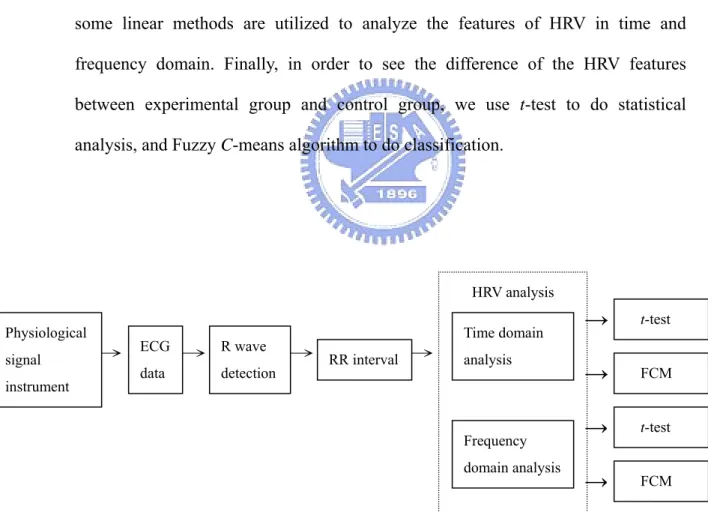
The methods adopted in this research are mainly to analyze electrocardiographic signals collected by noninvasive methods. The whole process of signal analysis is illustrated in Fig 3.1. The meaning of each block will be discussed in the following sections. The features of HRV will be analyzed after collecting ECG signals. Therefore the positions of R wave in ECG signals need to be detectedfirst, and then some linear methods are utilized to analyze the features of HRV in time and frequency domain. Finally, in order to see the difference of the HRV features between experimental group and control group, we use t-test to do statistical analysis, andFuzzy C-means algorithm to do classification.
→→ → → →
Fig 3.1 The processing procedure for ECG signal
HRV analysis Physiological signal instrument ECG data R wave detection RR interval Time domain analysis Frequency domain analysis t-test FCM t-test FCM
→
→
→
→
3.1 Physiological signal collecting system
The physiological signal collecting system in this research is shown as Fig 3.2. The physiological signals passing through adhesive electrodes attached to the body surface of a subject are amplified by BioAmp ( PowerLab ML136, biological signal amplifier ) made by ADInstruments. Next, signals are delivered to pc through USB interface, and built-in collecting software, chart4, takes record. The physiological signals which are measured synchronously include ECG, EMG, and GSR.
Fig.3.2 The physiological signal collecting system BioAmp
PowerLab
(ADInstruments ML136)
Physiological signal
Instrument
Bio Signal USB port
ECG signals measurement
In this research, we make use of bipolar limb lead I to do the work, collecting and processing of ECG signals. Then we connect lines to BioAmp made by ADInstruments to amplify ECG signals as shown in Fig.3.3. BioAmp has 3 different input ends; they are 2 differential input ends and 1 reference potential end respectively. In general, we put the reference on inner side of the right ankle, and positive and negative electrodes of two differential input ends on inner sides of left and right wrists respectively.
3.2 QRS detection and heart rate calculating
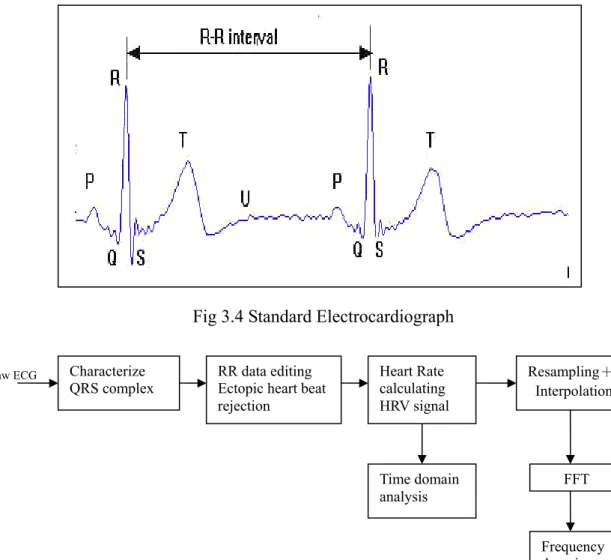
The magnitude of R wave is the biggest and the characteristic of R wave is the most obvious in ECG. (as shown in Fig 3.4) Generally speaking, in the analysis of heart rate, the position of QRS complex is needed to be detected at first, and then the position of the peak of R wave is found out by the setting of threshold. Next, the heart rate is calculated from R-R intervals, and the unreasonable heart rate signals must be rejected. (atria premature contractions and ventricular premature contractions) Thus, the heart rate variability can be obtained and the characteristics of HRV in time domain and frequency domain can be analyzed. The whole processing program is shown in Fig 3.5.
Fig 3.4 Standard Electrocardiograph
Fig 3.5 Flow chart of HRV analysis
Characterize
QRS complex Heart Rate calculating Resampling+ Interpolation HRV signal Raw ECG FFT Frequency domain analysis RR data editing
Ectopic heart beat rejection
Time domain analysis
3.2.1 Tompkins QRS detection algorithm
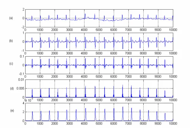
In this research, the QRS detection algorithm mainly bases on Tompkins QRS detection algorithm [32]. The algorithm includes 5 processes: band-pass filter, derivative, squaring, moving window integration, and adaptive thresholds (as shown in Fig 3.6). The signals after processing are shown in Fig. 3.7. After band-pass filtering, the amplitudes of P wave and T wave are suppressed due to their lower-frequency characteristics. The influences of baseline wander and high frequency noise are reduced. The main parts of the frequency response of QRS complexes are located in the main frequency band of the band pass filter; thus the QRS complexes are specially highlighted. In order to elevate the relative intensity of QRS complexes further, electrocardiographic signals are processed with differentiating and squaring to eliminate the influences of P wave and T wave on R wave. Then the signals dealt with the programs mentioned above are calculated with moving window integration so that each QRS complex corresponds to a signal peak. After using proper threshold detection, the correct position of the peak of R wave can be found. The detail explanations will be described as following.
Fig. 3.6 Tompkins QRS detection algorithm
Band-pass
filter derivative d /[] dt squaring[]2
Moving window integration
Adaptive threshold
Fig 3.7 Flow chart of R wave detection algorithm (a) Original signal (b) Output of band-pass filter (c) Output of differentiator (d) Output after squaring (e) Result after moving window-integration
(1) Bandpass Filter
The bandpass filter reduces the influence of muscle noise, 60 Hz interference, baseline wander, and T-wave interference. The desirable passband which maximizes the QRS energy is approximately 5-15 Hz. This class of filters having poles and zeros only on the unit circle permits limited passband design flexibility. Due to the sampling rate, we could not design a bandpass filter directly for the desired passband of 5-15 Hz using this specialized design technique. Therefore, we cascaded the low-pass and high-pass filters described below to achieve a 3 dB passband about 5-12 Hz, which reasonably close to the design goal. Fig 3.8 shows the result of the ECG signal with high frequency noise and baseline wander after passing through the bandpass filter.
Low-Pass Filter
The transfer function of the second-order low-pass filter is:
2 1 2 6 ) 1 ( ) 1 ( ) ( −− − − = z z z H (3.1) High-Pass Filter
The design of the high-pass filter is based on subtracting the output of a first-order low-pass filter from an all-pass filter. The transfer function for such a high-pass filter is:
) 1 ( ) 32 1 ( ) ( 16−1 32 − − + + + = z z z z H (3.2)
Fig 3.8(a) ECG signal with baseline wandering and high frequency noise interference (b) The same ECG signal after bandpass filter
(2) Derivative
After filtering, the signal is differentiated to provide the QRS-complex slope information. We use a five-point derivative with the transfer function:
) 2 2 1 )( 8 / 1 ( ) ( = − − −1 + −3 + −4 z z z z H (3.3) (3) Squaring Function
After differentiation, the signal is squared point by point. The equation of this operation is: ( ) [ ( )]2 n x n y = (3.4)
This makes all data points positive and does nonlinear amplification of the output of the derivative emphasizing the higher frequencies.
(4) Moving-Window Integration
The purpose of moving-window integration is to obtain waveform feature information about both the slope and the width of the QRS complex. In this research, the window is 24 samples wide. It is calculated from:
23)] -x(n 1) x(n ) (1/24)[x(n y(n)= + +…+ (3.5)
(5) Adjusting the Thresholds
The signal after moving window integration, its positions of R waves can be detected out by setting a proper threshold. Because the amplitude of electro- cardiographic signals is different from one to another, and there even exists difference in amplitude for the same subject, thus the setting of a threshold must be
the adaptivethreshold method for R-wave detection. The half mean value of first 3 QRS peaks is taken as the initial value,
threshold=(1/2)(1/3)(peak1+peak2+peak3)
(3.6) Then the new threshold is adjusted according to the new QRS peak. Its revising criterion is by equation (3.7)
new_threshold = new_value 0.5 × 0.1 + old_threshold × 0.9 (3.7)
The revising basis of new_threshold is made up of half 10% of the QRS peak detected latest, and the 90% of prior threshold so that thresholds can be compared, adjusted, and revised with the signal coming in continuously.
Fig. 3.9 Result of R wave Detection
3.2.2 Eliminating ectopic beats
To avoid ectopic beat such as PAC (premature atria contractions as shown in Fig 3-10(a)) and PVC (premature ventricular contractions as shown in Fig 3-10(b)),which will affect the normal heart rate spectrum analysis, we need to eliminate unreasonable ECG signals before calculating heart rate. Generally, ectopic heartbeat means that premature contraction of heart causes shorter heartbeat duration. Due to the compensatory effect, next heartbeat duration will be longer than normal interval. As shown in Fig 3-11(a), the sum of the successive RR intervals is smaller than two times of the normal RR interval (RR1+RR4>RR2+RR3). It is very important to deal with ectopic heartbeat during the period from recognizing R wave
position to calculating RR interval because even small amounts of ectopic heartbeat will have a negative influence on heart rate variability indexes of short term or long term recordings.
(a)
(b)
Fig.3.10 (a) premature atria contraction (PAC) (b) premature ventricular contraction (PVC)
The revising way of ectopic beat is to exclude the point where ectopic heartbeat happened. Then the duration is picked up from the last R wave peak to the next one, and choose the middle point of this duration as the new position of R wave peak shown in Fig 3-11(b). In the figure, R2 is ectopic beat (RR1 is much smaller than the average, and RR2 is opposite). According to the way mentioned above, R2 is excluded, and a new point Rn is inserted in the middle between R1 and R3. Then the interval between R1 and Rn becomes (1/2)(RR1+RR2).
(a)
(b)
Fig.3-11(a) Abnormal ECG signal (b) Modification of ectopic heartbeat
3.2.3 Heart rate calculating
When the position of the R wave peak is detected precisely, the time interval of successive R waves represents heartbeat period. The time series made up of every RR interval is called HRV signal shown in Fig 3.12. Because RR interval is different from one to another, thus, this signal is unequal sampled. However, the objects analyzed by digital signal processing are generally equal-sampled signals. Therefore this signal must be transformed to equal-sampled signal before using general digital signal processing methods.
In this research, we adopt window interpolations, which Berger used in 1986 to calculate HRV by equal sampling [3]. We first found out all RR intervals, and then decided the re-sampling frequency. The equation (3.8) represents the heart rate after re-sampling. 2 i r i n f r = × (3.8) i
r is the heart rate at the ith resample point, fr is re-sampling frequency, and n i
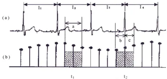
is the number of RR intervals that fell in the local window centered at the ith resample point. If re-sampling frequency is 5Hz, and original sampling frequency is 1000 Hz, there exists a new signal point separated by 200 sample points. Next we must get n , the number of RR intervals that fell in the local window centered at i every resample point. There are 2 conditions to decide n . As shown in Fig 3.13(a), i
if the sampling interval before the sample point and the one after the sample point are distributed in the same RR interval (I2 ), then n is a/ Ii 2. a is 2 sampling intervals ,that is, local window, and I2 is the second RR interval in Fig3.13(b). If the
sampling interval before the sample point and the one after the sample point are distributed in different RR intervals, then n should be decided by both of the RR i intervals. Thus n is b/Ii 3+c/I4. b and c are the time of sampling intervals distributed
in 2 different RR intervals respectively. We make use of the methods mentioned above to calculate all the values of n , and bring them into equation 3.8 so that the i
Fig. 3.13 Heart rate signal after equal sampling (a) a section of RR intervals (b) heart rate signal after equal sampling, when the center point of the local window falling at t1, n = a/ Ii 2, at t2 n = b/Ii 3+c/I4.
Fig. 3.14 Result after equal sampling (★is the point after re-sampling)
3.2.4 Heart rate variability analysis methods
The heart rate variability will be analyzed in time and frequency domain. The spectrum of HRV needs to be analyzed to distinguish the action of sympathetic from that of parasympathetic. Then the correlation between the characteristics of HRV and the action of autonomic nervous system also needs to be examined. Therefore, we transform the HRV signal from time domain to frequency domain by Fast Fourier Transform and find out the power spectrum so that we can observe the modulation of sympathetic and parasympathetic from the power spectrum of HRV.
According to the meaning of HRV and many kinds of measurement standardized proposed by the European Society of Cardiology and the North American Society of Pacing and Electrophysiology in 1996, some common analytic parameters in time and frequency domain will be introduced [11]. In these methods, the ECG signal records are classified into 2 kinds: short-term 5 minutes record and long-term 24 hours record.
1. Time domain analysis
For HRV in time domain analysis, the major analytic parameter is the mean and standard deviation of HRV for 5 minutes. They can be calculated by statistical methods. Time domain analysis is to detect each QRS complex interval in continuous ECG, and define it as RR interval (RRI). Table 3.1 lists the variables and measurement of the statistical methods in time domain. In the list, SDANN is proposed to do long-term 24 hours analysis. However, the methods of short-term analysis and those of long-term analysis can’t substitute each other, and they are adopted depending on the need of research. For HRV of short time 5 minutes, SDRR and RMSSD have better statistical meaning than pNN50 and NN50 do. Because this research is not a 24-hour record, SDRR and RMSSD are taken as reference indexes.
Table 3.1 Time domain parameters of HRV (*variables are the parameters adopted in this research)
Variable Unit Description
MRR* s Mean of RR intervals
SDRR* ms Standard deviation of all the RR intervals
SDANN ms Standard deviation of the mean values of all 5 minutes RR intervals in the
whole record
RMSSD* ms Root-Mean-Square values of the differences of all the successive RR intervals
NN50 count ms Counts of the differences which are larger than 50 ms in all the RR intervals
2. Frequency domain analysis
Frequency analysis of HRV is to do FFT on the RR intervals after equal sampling. As shown in Fig 3.15, the area under the power spectrum curve can express the power of frequency response. The total areas under the curve are total power. The area under each frequency band can express the power of that frequency band, so the response power in the very low frequency band is called very low frequency power (VLF); the response power in the low frequency band is called low frequency power (LFP); the response power in the high frequency band is called high frequency power (HFP). The magnitude of high frequency power can be seen as the index of parasympathetic activation. The magnitude of low frequency power can be seen as the index of co-mediation of both sympathetic and parasympathetic, and the ratio of high frequency power to low frequency one can be regarded as the index of activation balance of parasympathetic to sympathetic.
The spectrum components for short-term recording can be separated into 3 parts: VLF, LF, and HF. The power distribution and the center frequency of LF and HF are not fixed, but they may be affected by the modulation of autonomic nerves. The physiological meaning of VLF is seldom defined. The power of VLF, LF, and HF are usually calculated by absolute value (BPM2/Hz). LFP and HFP can be also expressed as normalized unit as shown in equation (3.9).
% 100 ) ( . ) ( × − = VLFpower Totalpower power HF LF u n orHF LF (3.9)
The normalized power of LF and HF expresses the mechanism behavior of control and balance of sympathetic and parasympathetic, and it may be seen as the relative value of evaluating LF(HF) power to total power. To describe the distribution of power spectrum completely, both absolute value and normalized value need to be calculated for comparing as shown in table 3.2. The magnitude of the power spectrum of VLF, LF, and HF bands, and the percentage occupied by them can show the mutual action of sympathetic and parasympathetic.
Table 3.2 Frequency domain parameters of HRV
Variable Unit Description
VLF Bpm2 Power in VLF range
LF Bpm2 Power in LF range
LF norm Nu LF power in normalized units LF/(total power - VLF)×100
HF Bpm2 Power in HF range
HF norm Nu HF power in normalized units HF/(total power - VLF)×100
3.3 Analysis of Poincare scattering plot
In this section, we will discuss how to make use of geometrical methods to observe heart rate variability. The method adopted is Poincare plot, which originally is a noun applied in astronomy, and it is a 2 dimensional scattering plot composed of current cardiac cycle length (the RR interval on the ECG) against the preceding RR interval. It reflects the variation of successive RR intervals, and it is a scattering plot marking the data positions of all the successive RR intervals in rectangular coordinate system. Poincare plot may not only show the whole features of HRV, but also visually display the instant variations of interbeat. Thus Poincare plot reveals the nonlinear characteristics of HRV [4,10].
◆Methods for constructing and analyzing the Poincare scattering plot
1. The drawing principle of Poincare scattering plot
By utilizing the suitable quantity of the RR intervals of the successive heartbeats, we set the first RRI as the abscissa value and the second RRI as the ordinate value of the first heart beat point. Then the second RRI is set as the abscissa value and the third RRI is set as the ordinate value of the second heart beat point. Then following in this order, abscissa is the collection of RR[n], and ordinate is the collection of RR[n+1]. Then after all heart beat points in some period are determined, Poincare scattering plot can be composed.
2. The analysis of typical patterns of Poincare scatter plot
The magnitude and regularity of HRV can be estimated from the area and shape of Poincare scatter plot. Generally speaking, according to the differences of the length distribution of RR intervals, Poincare plot can be classified by visual assessment into 4 typical patterns.
1) Comet shape
Figure 3.17 shows that RR intervals are located in the area of 500~1000 ms of 2 axes. Near the origin of the rectangular coordinate, the tail end is expanded symmetrically along the line of identity (slope=1) from the narrow bottom. The head end gets wider gradually, and the plot forms a unique comet pattern with big head and small tail. The scattering points most gather around the line of unitary slope passing through the origin. It expresses that the successive RR intervals are probably equal for normal people. The markings spreading around the angle of 45o presents the phenomenon of sinus arrhythmia. In figure 3.17, on the upper part of scattering plot, due to the slow heart rate, RR intervals are getting longer. It presents the serious extent of sinus arrhythmia. However, on the lower part of scattering plot, scattering plot is getting narrow gradually. It explains that when heart beats are increasing, sinus arrhythmia is going to a small extent. The length of the scatter plot along the direction of the angle of 45o represents the variation of the average heart rate. If the length is shorter, it represents that the variation of the average heart rate is small during the analysis period. The length of the line, along which scattering points spread, perpendicular to the line of identity represents the magnitude of the sharp variance of RR intervals. Generally speaking, the heavy density core of the scattering plot explains that successive RR intervals are nearly identical. It reflects the activation of sympathetic. The thin density part of the scattering plot represents
parasympathetic [4].
Fig. 3.17 Comet shape 2) Torpedo shape
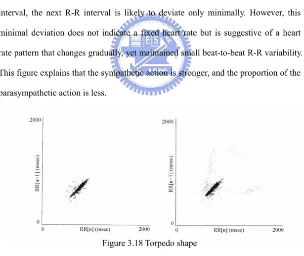
Figure 3.18 expresses a short torpedo-shaped scattering plot. For any R-R interval, the next R-R interval is likely to deviate only minimally. However, this minimal deviation does not indicate a fixed heart rate but is suggestive of a heart rate pattern that changes gradually, yet maintained small beat-to-beat R-R variability. This figure explains that the sympathetic action is stronger, and the proportion of the parasympathetic action is less.
Figure 3.18 Torpedo shape 3) Fan shape
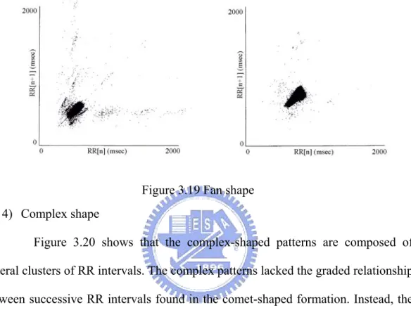
Figure 3.19 shows that points radiate in a relatively symmetric manner from a narrow base at the lower RR intervals. In the fan-shaped patterns, the overall range
of RR intervals is diminished, but the beat-to-beat RR interval dispersion is greater than that in comet-shaped patterns. The fan-shaped patterns have small increases in RR interval length that are associated with greater subsequent RR interval dispersion over a much shorter overall range.
Figure 3.19 Fan shape 4) Complex shape
Figure 3.20 shows that the complex-shaped patterns are composed of several clusters of RR intervals. The complex patterns lacked the graded relationship between successive RR intervals found in the comet-shaped formation. Instead, the complex configurations exhibited discrete stepwise clusters of points with distinct gaps between the clusters. The complex patterns may result from stepwise changes in RR intervals.
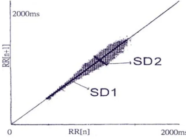
3. The quantitative analysis of Poincare scatter plot
Quantitative analysis entails fitting an ellipse to the scatter plot, with its center coinciding with the center point of the markings. The center point of the markings is at (RRaver,RRaver),where RRaver is the average RR-interval length for the
tachogram. The longest length of the line which passes through the center point along the line of identity is defined as the length of the Poincare cloud, that is SD1. It stands for the level of long-term HRV. The longest length of the line which passes through the center point perpendicular to the line of identity is defined as the width of the Poincare cloud, that is SD2. It indicates the level of short-term HRV [15].
Fig. 3.21 On the poincare plot, long-axis length is SD1 short-axis length is SD2
4. Mathematical relation of HRV indexes between Poincare plot and time domain [5] I. Time domain indices
The standard time domain measures of HRV are mentioned here again. Here the time-course of the RR intervals is denoted by RRn. The standard deviation of the
RR intervals, denoted by SDRR, is often employed as a measure of overall HRV. It is defined as the square root of the variance of the RR intervals
[ 2] 2
RR RR
E
SDRR= n − (3.10)
The standard deviation of the successive differences of the RR intervals, denoted by SDSD, is an important measure of short-term HRV. It is defined as the square root of the variance of the sequence △RRn = RRn-RRn+1(the delta-RR
intervals). [ 2] 2 n n RR RR E SDSD= ∆ −∆ (3.11)
Note that ∆RRn =E[RRn]−E[RRn+1]=0 for wide-sense stationary intervals. This
means RMSSD is statistically equivalent to SDSD. [( )2] 1 + − = =RMSSD E RRn RRn SDSD (3.12)
The Fourier transform of the autocorrelation function is the power spectrum of RR intervals. The autocorrelation function of the RR intervals is defined as
] [ ) ( n n m RR m =E RR RR + γ (3.13) Spectral analysis is normally performed on the mean-removed RR intervals and, therefore, the mean-removed autocorrelation function, called the auto-covariance function is often preferred
)] )( [( ) (m E RRn RR RRn m RR RR = − + − φ (3.14) For stationary RR intervals, the auto-covariance function is related to the autocorrelation function, as rightφRR(m)=γ(m)−RR2.
The auto-covariance function is related to the variance of the RR intervals as
SDRR2 = ψ RR(0), and the mean square of the successive differences,
RMSSD2 =2(γRR(0)-γRR(1))= 2(ψRR(0)-ψRR(1)).
II. Poincare plot descriptors
To characterize the shape of the plot mathematically, most researchers have used the technique of fitting an ellipse to the plot, as Fig 3.22 shows. A set of axis is oriented with the line-of-identity. The axis of the Poincare plot are related to the new