Copyright © 2006 Inderscience Enterprises Ltd.
Comparison of support-vector machines and
back propagation neural networks in forecasting
the six major Asian stock markets
Wun-Hua Chen and Jen-Ying Shih
Graduate Institute of Business Administration, National Taiwan University,No.1, Sec. 4, Roosevelt Road, Taipei 106, Taiwan, ROC Fax: 886-2-23654914
E-mail: [email protected] E-mail: [email protected]
Soushan Wu*
College of Management, Chang-Gung University, 259, Wen-Hwa 1st Road, Taoyuang, Taiwan, ROC E-mail: [email protected] *Corresponding author
Abstract: Recently, applying the novel data mining techniques for financial
time-series forecasting has received much research attention. However, most researches are for the US and European markets, with only a few for Asian markets. This research applies Support-Vector Machines (SVMs) and Back Propagation (BP) neural networks for six Asian stock markets and our experimental results showed the superiority of both models, compared to the early researches.
Keywords: financial forecasting; Support-Vector Machines (SVMs); Back
Propagation (BP) neural networks; Asian stock markets.
Reference to this paper should be made as follows: Chen, W-H., Shih, J-Y. and
Wu, S. (2006) ‘Comparison of support-vector machines and back propagation neural networks in forecasting the six major Asian stock markets’, Int. J.
Electronic Finance, Vol. 1, No. 1, pp.49–67.
Biographical notes: Wun-Hwa Chen received his PhD in Management
Science from the State University of New York at Buffalo in 1989. He is currently a Professor of Operations Management in the Department of Business Administration at National Taiwan University. His research and teaching interests lie in production planning and scheduling, AI/OR algorithmic design, data mining models for customer relationship management and mathematical financial modelling. He has published papers in numerous journals including
Annals of Operational Research, IEEE Transactions on Robotics and Automation, European Journal of Operational Research and Computers and Operations Research. In addition, he has held the Chairmanship in Information
Technology Advisory Committees of several government agencies in Taiwan and has extensive consulting experiences with many major corporations in Taiwan.
Jen-Ying Shih is a doctoral student in the Graduate Institute of Business Administration at National Taiwan University. Her current research interests include data mining and text mining for financial applications and management issues. She received her BS in Finance from National Taiwan University in 1995 and an MBA in Business Administration from National Taiwan University in 1997.
Soushan Wu received his PhD in Finance from the University of Florida in 1984. He is a Chair Professor and Dean of the College of Management, Chang-Gung University, Taiwan. He is also a visiting scholar at Clemson University, Hong Kong Polytechnic University. His research interests include management science, investment science, capital markets and information systems. He has published over 70 papers in Research in Finance, Financial Management,
Asia-Pacific Journal of Finance, International Journal of Accounting and Information Systems, etc. He has also served as an ad hoc reviewer for
academic journals in the fields of Accounting, Finance and Information Management. He serves as a Chief Editor of the Journal of Management (in Taiwan).
1 Introduction
In the business and economic environment, it is very important to accurately predict various kinds of financial variables to develop proper strategies and avoid the risk of potentially large losses. Few literature works have been devoted to the prediction of these variables, such as stock market return and risk prediction (Tay and Cao, 2001; Thomason, 1999b), sales forecasting (Steiner and Wittkemper, 1995) and monetary policy. However, stock markets are often affected by many factors in fundamental and technical analysis. In this situation, data mining techniques may be one of the ways to satisfy the demand for the accurate prediction of financial variables.
In the past, most prediction models were based on conventional statistical methods, such as time-series and multivariate analysis. In recent years, however, Artificial Intelligence (AI) methodologies, including the Artificial Neural Networks (ANNs), Genetic Algorithms (GA) and fuzzy technologies, have become popular research models. They have been applied to many financial realms, including economic indices prediction (Gestel et al., 2001; Leigh et al., 2002; Teixeira and Rodrigues, 1997; Zhang et al., 2001), stock/futures price prediction (Kamijo and Tanigawa, 1990; Tay and Cao, 2001), currency exchange rate prediction (Qi and Zhang, 2001; Shazly and Shazly, 1999), option trading (Bailey et al., 1998), bond rating (Kim and Han, 2001; Shin and Han, 2001), bankruptcy prediction (Lee et al., 1996; Zhang et al., 2001) and portfolio optimisation (Kosaka et al., 1991). These AI techniques were developed to meet the increasing demand for tools and methods that can predict, detect, classify and summarise the structure of variables and define the relationships between them – without relying too much on specific assumptions, such as linearity; or on error distributions, such as normality. Many AI applications in the financial analysis have addressed this demand by developing the parametric non-linear models.
In capital market research, stock or index prices are notoriously difficult to predict using the traditional forecasting methods, such as least squares regression, because of their chaotic nature. Consequently, several AI-based methodologies have been proposed that claim better prediction capabilities than traditional models. Most researches,
however, concentrated on the US and European capital markets; a very few studies have focused on the Asian capital markets, which are famous for their thin-dish-like characteristics, that is, they overreact to good or bad events, and are very volatile. In this paper, we apply two AI techniques, Back Propagation (BP) neural networks and Support Vector-Machines (SVMs), to construct the prediction models for forecasting the six major Asian stock market indices and compare the results with a benchmark developed by an autoregressive (AR) time-series model.
ANNs are a field of study within the AI area, where researchers employ a ‘biologically inspired’ method to process information. They are good for solving some real-world problems especially in the areas of forecasting and classification decisions. However, most of the research has learning pattern limitations because of the tremendous noise and complexity of the input data. Some research indicates that the BPs and SVMs can perform very well in the financial time-series forecasting, for example, BP algorithms have been applied as alternatives to statistical techniques because of their superior accuracy. On the other hand, SVMs deal with the non-linear function fitting problem very efficiently because they seek to minimise an upper bound of the generalisation error. Furthermore, they are unique, optimal and free from local minima. We therefore explore the applicability of BP and SVMs to the financial prediction problem.
The rest of this paper is organised as follows. In Section 2, previous research on financial prediction is reviewed. The two prediction methods used in this paper are discussed in Sections 3 and 4. Our research data and modelling are presented in Section 5 and our empirical results are given in Section 6. Finally, in Section 7, we present our conclusions.
2 Related works
2.1 Review of conventional structural models
Many models have been developed to predict stock market behaviour, for example, one-or multi-step ahead price prediction, price change direction, returns and risks, portfolio asset allocation and trading strategy decisions. Structural models are the major approach in the stock market prediction. Two renowned models are: the Capital Asset Pricing Model (CAPM) (Sharpe, 1964), which describes the relationship between an individual stock return – including its risk – and the market return; and the Arbitrage Pricing Theory (APT) (Roll and Ross, 1980), which describes the relationship between an individual stock return and some macroeconomic variables. In addition, Brock et al. (1992) found non-linearities in market prices and showed that the use of technical analysis indicators, under certain assumptions, may generate efficient trading rules (Brock et al., 1992). The prices of other financial commodities also have this non-linear dynamic property. Savit (1989), for example, suggested a non-linear dynamic model for option prices.
In the last decade, statistical models, especially time-series models and multivariate models, have become very popular in the construction of various kinds of stock market behaviour prediction models, as well as the economic indicator models. With regard to time-series models, Granger and Sin (2000) proposed AR- and ARCH-like models for exploring the predictability of an alternative measure of risk. Also, Östgermark and
Hernesniemi (1995) measured the influence of the freshness of information on the ability of an investor to forecast a stock index and the stock index future by applying vector models, known as VARMAX-models. This study used data from the Finnish FOX index, depicting price movements of the Helsinki Stock Exchange and the FOX futures index (Östgermark and Hernesniemi, 1995).
Most multivariate analytical prediction models choose some critical determinants as input variables to predict stock market behaviour and try to detect the relationships between the input and output variables, such as stock return, risk, etc. The choice of the input variables is somewhat arbitrary, as there is no formal theory that supports stock returns as a function of micro- and macroindices. The former includes some technical analytical indicators, while the latter includes interest rates, Gross Domestic Production (GDP), etc. The representative models of multivariate analytical prediction models are linear regression models and multivariate discriminant analytical models (Baestaens and van de Bergh, 1995; Chen et al., 1986; Ferson and Harvey, 1991).
2.2 AI models
Conventional statistical models have had limited success, primarily because the structural relationship between an asset price and its determinants changes over time; hence, AI has become more popular in the capital market research in the recent years. A number of models use AI to forecast the price behaviour of the financial commodities and compare the results with the traditional statistical methodologies or the price behaviour of derivative financial commodities. Refenes et al. (1995), for example, modelled stock returns with ANNs in the framework of APT and compared their study with regression models. They showed that even the simple neural learning procedures, such as BP algorithms easily outperform the best practice of regression models in a typical stock ranking application within the framework of APT. Tsibouris and Zeidenberg (1995) applied two models, a BP model and a temporal difference model, to six stock returns to test the weak form of Efficient Market Hypothesis (EMH). They found some evidence to question the null hypothesis that the stock market is weakly efficient. Steiner and Wittkemper (1995) investigated the performance of several ANN models that forecast the return of a single stock and showed that ANNs outperform comparable statistical techniques in this area. They reported that the relationship between the return of a stock and factors of the capital market is usually non-linear and may contain dependencies in time. There may also be multiple connections between several factors (Steiner and Wittkemper, 1995).
Shazly and Shazly (1999) suggested a hybrid system combining neural networks and genetic training to forecast the three-month spot rate of exchange for four currencies: the British pound, the German mark, the Japanese yen and the Swiss franc. The performance of the model seems to be better than the predictions made by the forward and futures rates (Shazly and Shazly, 1999). Tay and Cao (2001) applied SVMs to the price prediction of five real futures contracts from the Chicago Mercantile Market. Their objective was to examine the feasibility of using SVMs in financial time-series forecasting by comparing them with a multilayer BP neural network. On the basis of some deviation and direction performance criteria, the results show that the SVM outperforms the BP neural network (Tay and Cao, 2001). Gestel et al. (2001) applied the Bayesian evidence framework, already used successfully in the design of multilayer perceptions, for Least Squares SVM (LS-SVM) regression to infer non-linear models for
predicting a time-series and the related volatility. They applied the model to the prediction of the US short-term interest rate and the DAX 30 index, and compared the results with the time-series models, such as AR and GARCH (1,1) and buy and hold strategies. LS-SVM outperformed the other models in terms of the percentage of correct sign predictions by 5–8% (Gestel et al., 2001).
Wittkemper and Steiner (1996) used financial statements from 67 German corporations for the period 1967–1986 to predict a stock’s systematic risk by different methods, including the traditional methods such as the Blume and Fund models, neural network models and GA models. They showed that the neural networks, whose topologies had been optimised by a genetic algorithm, gave the most precise forecasts.
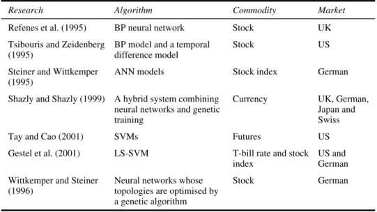
Although the superiority of the AI models has been shown in the US and European financial markets, few researches have been carried out in Asian markets (see Table 1). As it is not possible to generalise the superiority of a single AI model for all markets, we designed two AI models to examine time-series forecasting in the six major Asian stock markets as listed earlier, some of which are renowned for their thin-dish-like characteristics.
Table 1 Research into the superiority of AI models
Research Algorithm Commodity Market
Refenes et al. (1995) BP neural network Stock UK
Tsibouris and Zeidenberg (1995)
BP model and a temporal difference model
Stock US
Steiner and Wittkemper (1995)
ANN models Stock index German
Shazly and Shazly (1999) A hybrid system combining neural networks and genetic training
Currency UK, German,
Japan and Swiss
Tay and Cao (2001) SVMs Futures US
Gestel et al. (2001) LS-SVM T-bill rate and stock index
US and German Wittkemper and Steiner
(1996)
Neural networks whose topologies are optimised by a genetic algorithm
Stock German
3 SVMs for time-series forecasting
3.1 Introduction to SVMs
The SVM, which originated as an implementation of Vapnik’s Structural Risk Minimization (SRM) principle (Vapnik, 1995), is now being used to solve a variety of learning, classification and prediction problems. In many ways, an SVM performs the same function as an ANN. For example, when both the input and output data are available (supervised learning in ANN), the SVM can perform classification and regression; but when only the input data are available, it can perform clustering,
density estimation and principle component analysis. The SVM is more than just another algorithm. It has the following advantages over an ANN:
1 it can obtain the global optimum
2 the overfitting problem can be easily controlled and
3 empirical testing has shown that the performance of SVMs is better than ANNs in classification (Cai and Lin, 2002; Morris, and Autret, 2001) and in regression (Tay and Cao, 2001).
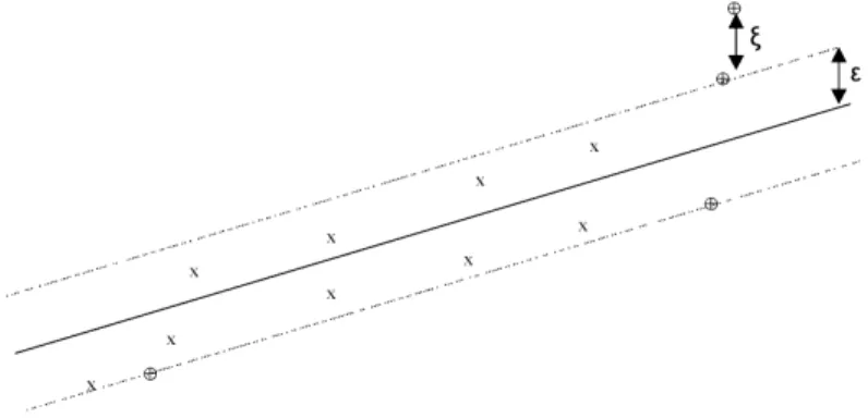
The SVM deals with classification and regression problems by mapping the input data into high-dimensional feature spaces. Its central feature is that the regression surface can be determined by a subset of points or Support-Vectors (SV); all other points are not important in determining the surface of the regression. Vapnik introduced a ε-insensitive zone in the error loss function (Figure 1). Training vectors that lie within this zone are deemed correct, whereas those that lie outside the zone are deemed incorrect and contribute to the error loss function. As with classification, these incorrect vectors also become the support-vector set. Vectors lying on the dotted line are SV, whereas those within the ε-insensitive zone are not important in terms of the regression function.
Figure 1 Approximation function (solid line) of the SV regression using a ε-insensitive zone (the area between the dotted lines)
3.2 Support-vector regression
Here, we introduce the most important features of Support-Vector Regression (SVR). Firstly, we discuss the simplest model of SVR, a linear regression in the feature space. Though it is the easiest algorithm but usually not very useful in real-world applications, it is a key for understanding complex SVR models. This is followed by a discussion of the kernel functions that deal with non-linear decision surfaces. A discussion of SVMs is given by Burges (1998), Cristianini and Taylor (2000) and Smola and Scholkopf (1998).
SVR is based on a similar concept to SVM classifiers. By generalising the SVM algorithm for regression estimation, the SVR algorithm tries to construct a linear function such that the training points lie within a distance ε (Figure 1). As with SVM classifiers, we can also derive a quadratic programming problemto generalise non-linear regression by using the kernel functions.
Given a set of training data
{
( , ),...,x y1 1(
x yl, l)
}
⊂ × , where X denotes the space ofX R the input patterns, the goal of SVR is to find a function ( )f x that has at most ε deviation from the targetsy for all of the training data and, at the same time, is as flat as possible.iLet the linear function f takes the form:
T
( ) with ,
f x =w x+b w∈X b∈R (1)
Flatness in (1) means a smaller w . The problem can be formulated as
2 T T 1 min 2 s.t. i i i i w y w x b w x b y ε ε − − ≤ + − ≤ (2)
However, not all the problems are feasible in this hard margin. As with the classification problem, non-negative slack variables, ξ ξ can be introduced to deal with thei, i*, otherwise infeasible constraints of the optimisation problem (2). Thus, the formation is stated as
(
)
2 * 1 T T * * 1 min 2 s.t. , 0 l i i i i i i i i i i i w C y w x b w x b y ξ ξ ε ξ ε ξ ξ ξ = + + − − ≤ + + − ≤ + ≥ ∑
(3)The constant C > 0 determines the error margin trade-off between the flatness of f and the amount of deviation larger than ε that is tolerated. The formulation corresponds to a
-insensitive
ε loss function ξ described byε,
0 if otherwise ε ξ ε ξ ξ ε ≤ = − (4)
The Lagrange relaxation of (3) is as follows:
2 * T 1 1 * * T * * 1 1 1 ( ) ( ) 2 ( ) ( ) l l i i i i i i i i l l i i i i i i i i i i L w C y w x b y w x b ξ ξ α ε ξ α ε ξ η ξ η ξ = = = = = + + − + − + + − + + − − − +
∑
∑
∑
∑
(5)where α α ηi, i*, iandη are Lagrange multipliers. Thus, the dual optimisation problem ofi* (5) is as follows:
(
)
(
)
(
)
* * T * * , 1 1 1 * 1 * 1 max ( )( ) 2 0 s.t. , [0, ] l l l i i j j i j i i i i i i j i i l i i i i i x x y C α α α α ε α α α α α α α α = = = = − − − − + + − − = ∈ ∑
∑
∑
∑
(6)Equation (1) can now be rewritten as follows:
(
*)
(
*)
T 1 1 and therefore ( ) l l i i i i i i i i w α α x f x α α x x b = = =∑
− =∑
− + (7)w is determined by training patterns x which are SVs. In a sense, the complexity of thei, SVR is independent of the dimensions of the input space because it only depends on the number of SV.
To enable the SVR to predict a non-linear situation, we map the input data into a feature space. The mapping to the feature space F is denoted by
: ( ) n F x x Φ ℜ → Φ 6
The optimisation problem (6) can be rewritten as follows:
(
)
(
)
(
)
* * T * * , 1 1 1 * 1 * 1 max ( )( ) ( ) ( ) 2 0 s.t. , [0, ] l l l i i j j i j i i i i i i j i i l i i i i i x x y C α α α α ε α α α α α α α α = = = = − − − Φ Φ − + + − − = ∈ ∑
∑
∑
∑
(8)The decision function can be computed by the inner products of T
( )x ( )xi
Φ Φ without
explicitly mapping to a higher dimension, which is a time-consuming task. Hence, the kernel function is as follows:
T
( , ) ( ) ( ) K x z ≡ Φ x Φ z
By using a kernel function, it is possible to compute the SVR without explicitly mapping in the feature space. The condition for choosing kernel functions should conform to Mercers condition, which allows the kernel substitutions to represent dot products in some Hilbert space.
4 ANNs for time-series forecasting
4.1 Introduction to ANNs
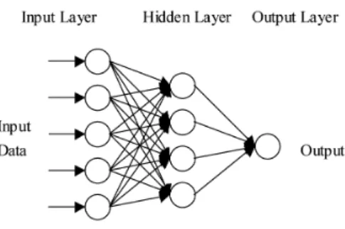
An ANN is a biologically inspired form of distributed computation. It simulates the functions of the biological nervous system by a composition of interconnected simple elements (artificial neurons) operating in parallel, as shown in Figure 2. An element is a simple structure that performs three basic functions: input, processing and output. ANNs can be organised into several different connection topologies and learning algorithms (Lippmann, 1987). The number of inputs to the network is constrained by the problem type, whereas the number of neurons in the output layer is constrained by the number of outputs required by the problem type. However, the number of hidden layers and the sizes of the layers are decided by the designer.
Figure 2 A neural network with one hidden layer
ANNs have become popular because they can be generalised and do not make any assumption about the underlying distribution of data. In addition, they have the ability to learn any function, for example, the two-layer sigmoid/linear network can represent any functional relationship between the input and output if the sigmoid layer has enough neurons. ANNs have been successfully applied in different areas, including marketing, retail, banking and finance, insurance telecommunications and operations management (Smith and Gupta, 2000).
ANNs apply many learning rules, of which BP is one of the most commonly used algorithms in financial research. We therefore use the BP to develop ANN models in this paper. In the next section, we discuss the BP neural networks.
4.2 Back Propagation
BP trains multilayer feedforward networks with differentiable transfer functions to perform function approximation, pattern association and pattern classification. It is the process by which the derivatives of network error, with respect to network weights and biases, are computed to perform computations backwards through the network. Computations are derived using the chain rule of calculus.
There are several different BP training algorithms with a variety of different computation and storage requirements. No single algorithm is best suited to all the problems. All the algorithms use the gradient of the performance function to determine how to adjust the weights to minimise the performance. For example, the performance function of feed forward networks is the Mean Square Error (MSE).
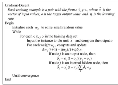
The basic BP algorithm adjusts the weights in the steepest descent direction (negative of the gradient); that is, the direction in which the performance function decreases most rapidly. The training process requires a set of examples of proper network inputs and target outputs. During the training, the weights and biases of the network are iteratively adjusted to minimise the network performance function. Figure 3 represents the pseudocode of a BP training algorithm.
Figure 3 Gradient-descent algorithm
For the function approximation problems in networks that contain up to a few hundred weights, the Levenberg–Maruardt algorithm generally has the fastest convergence. This advantage is especially useful if a very accurate training is required.
One method for improving generalisation is early stopping, which divides the available training samples into two subsets:
1 the training set, used for computing the gradient and updating the network weights and biases
2 the validation set, the error of the validation set, which is monitored during the training process, will normally decrease during the initial phase of training, as does the training set error.
However, it typically increases when the network begins to overfit the data. After it has increased for a specified number of iterations, the training is stopped, and the weights and biases at the minimum of the validation error are returned.
5 Results of empirical testing
5.1 Data sets
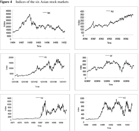
We examined the six major Asian stock market indices in our experiment, namely the Nikkei 225 (NK), the All Ordinaries (AU), the Hang Seng (HS), the Straits Times (ST), the Taiwan Weighted (TW) and the KOSPI (KO). Data were collected from the Yahoo Finance, the Taiwan Stock Exchange and the Korean Stock Exchange. The time periods
used and the indices’ statistical data are listed in Table 2, and the daily closing prices used as the data sets are plotted in Figure 4. The time periods cover many important economic events, which we believe are sufficient for the training models.
Table 2 Description of data sets
Index Symbol Time period High Low Mean SD
Nikkei 225 NK 1984/1/4–2002/5/31 38,916 9420 19,433 6297.33 All Ordinaries AU 1984/8/3–2002/5/31 3440 712.40 2019.48 728.20 Hang Seng HS 1986/12/31–2002/5/31 18,301.69 1894.90 8214.55 4459.14 Straits Times ST 1987/12/28–2002/5/31 2582.94 805.04 1713.89 423.25 TAIEX TW 1971/1/5–2002/5/31 12,495.34 116.48 2819.70 3030.77 KOSPI KO 1980/1/4–2002/5/31 1138.75 93.1 516.33 317.58
Figure 4 Indices of the six Asian stock markets
We further transformed the original closing price into a five-day Relative Difference in Percentage of price (RDP). According to Thomason (1999a,b) and Tay and Cao (2001), this transformation has many advantages. The most important is that the distribution of the transformed data becomes more symmetrical so that it follows a normal distribution
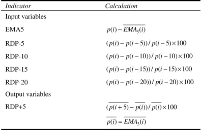
more closely. This improves the predictive power of the neural network. Following the prediction model used in the previous research (Tay and Cao, 2001; Thomason, 1999a,b), the input variables in this paper are determined from four-lagged RDP values based on five-day periods (RDP-5, RDP-10, RDP-15 and RDP-20); and one transformed closing index (EMA5), obtained by subtracting a five-day exponential moving average from the closing indices (Table 3). Applying the RDP transform to the closing indices over the period of the data removes the trend in prices. EMA5 is used to retain as much information as possible from the original closing index because the application of the RDP transform to the original closing index may remove some useful information. The five-day-based input variables correspond to technical analysis concepts. The output variable RDP+5 is obtained by first smoothing the closing index with a three-day exponential moving average. The application of a smoothing transform to the dependent variable generally enhances the prediction performance of the neural network (Thomason, 1999b).
Table 3 Input and output variables
Indicator Calculation Input variables EMA5 p i( )−EMA i5( ) RDP-5 ( ( )p i −p i( −5)) / (p i− ×5) 100 RDP-10 ( ( )p i −p i( −10)) / (p i−10) 100× RDP-15 ( ( )p i −p i( −15)) / (p i−15) 100× RDP-20 ( ( )p i −p i( −20)) / (p i−20) 100× Output variables RDP+5 ( (p i+ −5) p i( )) / ( ) 100p i× 3 ( ) ( ) p i =EMA i
5.2 Preprocessing data and design of the models
Firstly, RDP values beyond the ±2 Standard Deviations (SD) are selected as outliers and replaced with the closest marginal values. Next, the preprocessing technique for data scaling is performed. For the sake of comparison across data sets, all data points are scaled in the range of –1 to 1, including the output data. Each of the six data sets is partitioned into three subsets according to the time sequence in the ratio 80:10:10. The first part is used for training; the second is a validating set that selects optimal parameters for the SVR and prevents the overfitting found in the BP neural networks and the last part is used for the testing.
5.3 Performance criteria
Although the MSE is a perfectly acceptable measure of performance, in practice the ultimate goal of any testing strategy is to confirm that the results of models are robust and capable of measuring the profitability of a system. It is important, therefore, to
design a test from the outset. This is not always carried out with the level of rigor that it merits, partly because of unfamiliarity with the established methods or practical difficulties intrinsic to non-linear systems. Consequently, we designed test sets to evaluate the effects of the models.
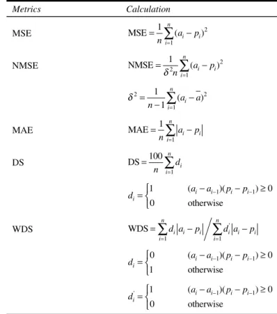
According to Tay and Cao (2001) and Thomason (1999a,b), the prediction performance is evaluated using the following statistics: MSE, Normalised Mean Squared Error (NMSE), Mean Absolute Error (MAE), Directional Symmetry (DS) and Weighted Directional Symmetry (WDS). These criteria are defined in Table 4. MSE, NMSE and MAE measure the correctness of a prediction in terms of levels and the deviation between the actual and predicted values. The smaller the values, the closer the predicted time-series values will be to the actual values. Although predicting the levels of price changes (or first differences) is desirable, in many cases the sign of the change is equally important. Most investment analysts are usually far more accurate at predicting directional changes in an asset price than predicting the actual level. DS provides an indication of the correctness of the predicted direction of RDP+5 given in the form of percentages (a large value suggests a better predictor). WDS measures both the magnitude of the prediction error and its direction. It penalises incorrectly predicted directions and rewards directions that are correctly predicted. The smaller the value of WDS, the better the forecasting performance will be in terms of both the magnitude and direction.
Table 4 Performance metrics and their calculation
Metrics Calculation MSE 2 1 1 MSE ( ) n i i i a p n = =
∑
− NMSE 2 2 1 1 NMSE ( ) n i i i a p n δ = =∑
− 2 2 1 1 ( ) 1 n i i a a n δ = = − −∑
MAE 1 1 MAE n i i i a p n = =∑
− DS 1 100 DS n i i d n = =∑
1 1 1 ( )( ) 0 0 otherwise i i i i i a a p p d = − − − − ≥ WDS ' 1 1 WDS n n i i i i i i i i d a p d a p = = =∑
−∑
− 1 1 0 ( )( ) 0 1 otherwise i i i i i a a p p d = − − − − ≥ 1 1 ' 1 ( )( ) 0 0 otherwise i i i i i a a p p d = − − − − ≥ 5.4 SVM implementation
We applied Vapnik’s SVM for regression by using LIBSVM (http://www.csie. ntu.edu.tw/~cjlin/libsvm/). The typical kernel functions used in SVRs are the polynomial kernel ( , )k x y = (x× +y 1)d and the Gaussian kernel k x y( , )=exp
(
−1/δ2(x−y)2)
,where d is the degree of the polynomial kernel and δ 2
is the bandwidth of the Gaussian kernel. We chose the Gaussian kernel as our kernel function because it performs well under general smoothness assumptions.
The parameters to be determined are kernel bandwidth 2
,
δ C and .ε According to Thomason (1999a,b) and Tay and Cao (2001), it showed that SVRs are insensitive to ,ε as long as it is a reasonable value. Thus, we chose 0.001 for .ε For δ and C, we used2
tenfold cross validation to choose suitable values. The values of the candidates were 2
{2,1, 0.5, 0.1, 0.01, 0.001, 0.0001}
δ ∈ and C∈{500,250,100, 50,10,2}, respectively.
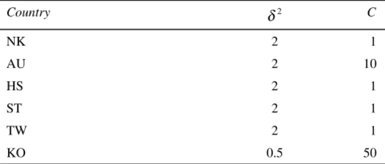
Table 5 gives the parameters obtained from the trials of each market scenario.
Table 5 Parameter set of each index
Country 2 δ C NK 2 1 AU 2 10 HS 2 1 ST 2 1 TW 2 1 KO 0.5 50 5.5 BP implementation
The BP models used in this experiment are implemented using the Matlab 6.1’s ANN toolbox. Several learning techniques, such as the quasi-Newton method, Levenberg-Marquardt algorithm and conjugate gradient methods could also be used. For efficiency, however, we use the Levenberg–Marquardt algorithm. The architecture of the BP model is as follows: the number of hidden nodes varies from 8 to 20 and the optimum number of hidden nodes (10) that minimises the error rate on the validation set is determined. The activation function of the hidden layer is sigmoid and the output node uses the linear transfer function.
6 Results and discussion
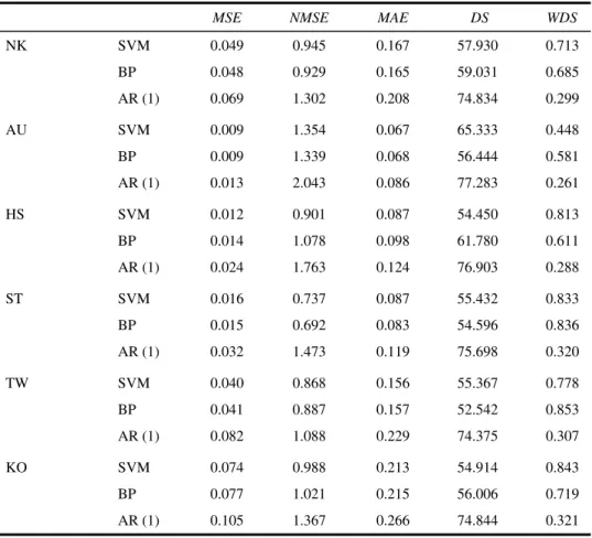
For each market, we also designed an AR (1) time-series model as the benchmark for comparison. The forecasting results of the SVM, BP and AR (1) for the test set are collated in Table 6. In general, SVMs and BP models outperformed the AR (1) model in the deviation performance criteria. However, in the direction performance criteria, the AR (1) model proved superior, possibly because SVMs and BPs are trained in terms of
deviation performance; the former to find the error bound and the latter to minimise MSE. Thus, in the deviation performance criteria, they perform better than the benchmark model AR (1). With regard to the direction criteria, the time-series model has an intrinsic merit because it emphasises the trend of the series. Therefore, the two AI models cannot outperform AR in the direction criteria in the six Asian markets under study.
Table 6 Comparison of the results of SVM, BP and AR (1) model on the test set
MSE NMSE MAE DS WDS
NK SVM 0.049 0.945 0.167 57.930 0.713 BP 0.048 0.929 0.165 59.031 0.685 AR (1) 0.069 1.302 0.208 74.834 0.299 AU SVM 0.009 1.354 0.067 65.333 0.448 BP 0.009 1.339 0.068 56.444 0.581 AR (1) 0.013 2.043 0.086 77.283 0.261 HS SVM 0.012 0.901 0.087 54.450 0.813 BP 0.014 1.078 0.098 61.780 0.611 AR (1) 0.024 1.763 0.124 76.903 0.288 ST SVM 0.016 0.737 0.087 55.432 0.833 BP 0.015 0.692 0.083 54.596 0.836 AR (1) 0.032 1.473 0.119 75.698 0.320 TW SVM 0.040 0.868 0.156 55.367 0.778 BP 0.041 0.887 0.157 52.542 0.853 AR (1) 0.082 1.088 0.229 74.375 0.307 KO SVM 0.074 0.988 0.213 54.914 0.843 BP 0.077 1.021 0.215 56.006 0.719 AR (1) 0.105 1.367 0.266 74.844 0.321
The performances of the SVM and BP models are fairly good compared to Tay and Cao (2001). The deviation criteria, such as NMSEs are less than 1, except for the AU index in the SVMs. The NMSEs of BP are less than 1, except for the AU and KO indices. As to the correctness of predicted direction, all the values of DS are more than 50%. We also obtain smaller WDS values.
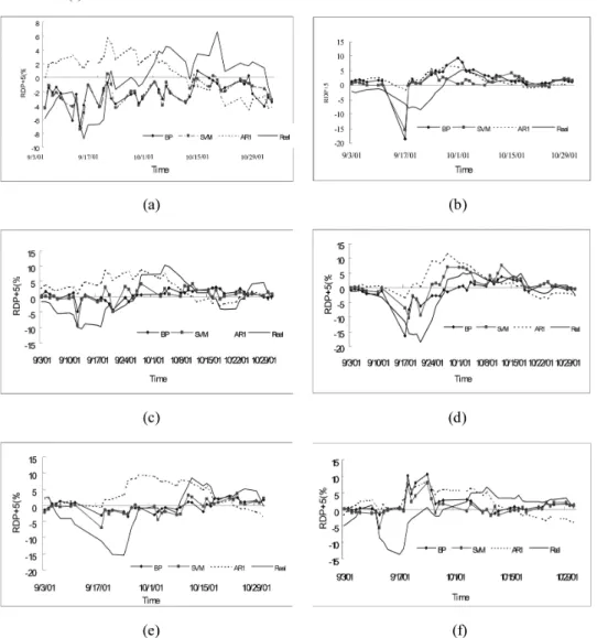
Figure 5 shows the predicted effects for the period September–October 2001, which included the 9/11 terrorist attacks. The fitted lines of the BP and SVM models seem close to each other and both are closer to the real value line than the AR (1) line because of the smaller values of the deviation measurement. However, their direction performance is not as good as the AR (1) line for the smaller value of the direction measurement in the SVM and BP models.
Figure 5 RDP+5 values of indices fitted by AR (1), BP and SVM models and their real values. (a) Nikkei 225, (b) All Ordinaries, (c) Hang Seng, (d) Straits Times, (e) TAIEX and (f) KOSPI
Table 7 gives the comparison of the results of the BP and SVM models. There is no difference in the AU index for the three deviation performance criteria (MSE, NMSE and MAE). In the HS, TW and KO data sets, the SVM models perform slightly better than the BP models. On the other hand, the BP method performs only a little better than SVMs in the NK and ST data sets. In total, there is no significant difference between the performances of the two models in the deviation measurements. Taking the AR (1) model as a benchmark to evaluate the two AI models, both seem to perform better than AR (1) for all six markets in terms of the deviation measurements. For the other two predicted direction criteria (DS and WDS), SVMs work better than BPs in the AU, ST and TW indices; however, BPs work better than SVMs in the NK, HS and KO indices. In all six markets, we find that the AR (1) model outperforms the SVM and BP models in terms of the predicted direction criteria.
Because there is no consistency in the superiority of the two AI models, our result differs from that of Tay and Cao (2001). The performance of SVMs is not always better than the BPs in these performance criteria. Table 7 summarises the comparison between the two models. Generally speaking, based on the five performance criteria, SVMs fit the AU, HS, TW and KO indices well, whereas BP fits NK and ST indices.
Table 7 Comparison of BP and SVMs on the test set
MSE NMSE MAE DS WDS Summary
NK − − − − − − AU 0 − + + + + HS + + + − − + ST − − − + + − TW + + + + + + KO + + + − − +
‘0’ represents no difference between SVM and ANN, ‘+’ represents SVMs that perform well and ‘–’ represents ANNs that perform well.
7 Conclusion
In this paper, we have examined the feasibility of applying two AI models, SVM and BP, to financial time-series forecasting for the Asian stock markets, some of which are famous for their thin-dish-like characteristics. Our experiments demonstrate that both models perform better than the benchmark AR (1) model in the deviation measurement criteria. Although previous research claims that the SVM method is superior to the BP, there are some exceptions, for example, the NK and the ST indices. In general, the SVM and the BP models perform well in the prediction of indices behaviour in terms of the deviation criteria. Our experiments also show that the AI techniques can assist the stock market trading and the development of the financial decision support systems.
Future research should apply more complex SVM methods and other ANN algorithms to the forecasting of Asian stock markets. Direction prediction criteria are important signals in the trading strategies of investors. Improving these criteria in AI models is, therefore, another important issue in the financial research. In our current models, we only select the return of index price information as input variables. Enhancing the performance of prediction models by including other efficient input variables (such as some macroeconomic variables), the relationships between different markets and other trading information about the markets should also be the subject of future research.
References
Anthony, M. and Biggs, N.L. (1995) ‘A computational learning theory view of economic forecasting with neural nets’, Neural Networks in the Capital Markets, pp.77–98.
Baestaens, D.E. and van den Bergh, W.M. (1995) ‘Tracking the Amsterdam stock index using neural networks’, Neural Networks in the Capital Markets, pp.149–161.
Bailey, D.B., Tompson, D.M. and Feinstein, J.L. (1988) ‘Option trading using neural networks’, in J. Herault and N. Giamisasi (Eds). Proceedings of the International Workshop, Neural
Networks and their Applications, Neuro-Times, 15–17 November, pp.395–402.
Brock, W.A., Lakonishok, J. and Baron, B.L. (1992) ‘Simple technical trading rules and the scholastic properties of stock return’, Journal of Finance, Vol. 27, No. 5, pp.1731–1764. Burges, C.J.C. (1998) ‘A tutorial on support vector machines for pattern recognition’, Data Mining
and Knowledge Discovery, Vol. 2, No. 2, pp.1–47.
Cai, Y-D. and Lin, X-J. (2002) ‘Prediction of protein structural classes by support vector machines’, Computers and Chemistry, Vol. 26, pp.293–296.
Chen, N-F., Roll, R. and Ross, S.A. (1986) ‘Economic forces and the stock market’, Journal of
Business, Vol. 59, No. 3, pp.383–403.
Cristianini, N. and Taylor, J.S. (2000) An Introduction to Support Vector Machines and Other
Kernel-Based Learning Methods, Cambridge University Press.
Ferson, W.A. and Harvey, C.R. (1991) ‘Sources of predictability in portfolio returns’, Financial
Analysts Journal, Vol. May–June, Vol. 47, No. 3, pp.49–56.
Gestel, T.V., Suykens, J.A.K., Baestaens, D-E., Lambrechts, A., Lanckriet, G., Vandaele, B., Moor, B.D. and Vandewalle, J. (2001) ‘Financial time-series prediction using least squares support vector machines within the evidence framework’, IEEE Transactions on Neural
Networks, Vol. 12, No. 4, pp.809–821.
Granger, C.W.J. and Sin, C.Y. (2000) ‘Modeling the absolute returns of different stock indices: exploring the forecastability of an alternative measure of risk’, Journal of Forecast, Vol. 19, pp.277–298.
Kamijo, K.I. and Tanigawa, T. (1990) ‘Stock price recognition – a recurrent neural network approach’, Proceedings of the International Joint Conference on Neural Networks, Vol. I, pp.215–221.
Kim, K-S. and Han, I. (2001) ‘The cluster-indexing method for case-based reasoning using self-organizing maps and learning vector quantization for bond rating cases’, Expert Systems
with Applications, Vol. 21, pp.147–156.
Kosaka, M., Mizuno, H., Sasaki, T., Someya, R. and Hamada, N. (1991) ‘Applications of fuzzy logic and neural networks to securities trading decision support system’, Proceedings of the
IEEE International Conference on Systems, Man and Cybernetics, pp.1913–1918.
Lee, K.C., Han, I. and Kwon, Y. (1996) ‘Hybrid neural network models for bankruptcy predictions’, Decision Support Systems, Vol. 18, pp.63–72.
Leigh, W., Purvis, R. and Ragusa, J.M. (2002) ‘Forecasting the NYSE composite index with technical analysis, pattern recognizer, neural network, and genetic algorithm: a case study in romantic decision support’, Decision Support Systems, Vol. 32, pp.361–377.
Lippmann, R.P. (1987) ‘An introduction to computing with neural nets’, IEEE ASSP Magazine, April, pp.36–54.
Morris, C.W. and Autret, A. (2001) ‘Support vector machines for identifying organisms – a comparison with strongly partitioned radial basis function networks’, Ecological Modeling, Vol. 146, pp.57–67.
Östgermark, R. and Hernesniemi, H. (1995) ‘The impact of information timeliness on the predictability of stock and futures returns: an application of vector models’, European Journal
of Operational Research, Vol. 85, pp.111–131.
Qi, M. and Zhang, G.P. (2001) ‘An investigation of model selection criteria for neural network time-series forecasting’, European Journal of Operational Research, Vol. 132, pp.666–680. Refenes, A-P., Zapranis, A.D. and Francis, G. (1995) ‘Modeling stock returns in the framework of
APT: a comparative study with regression models’, Neural Networks in the Capital Markets, pp.101–125.
Roll, R. and Ross, S. (1980) ‘An empirical investigation of the arbitrage pricing theory’, Journal of
Finance, Vol. 35, No. 5, pp.1073–1103.
Savit, R. (1989) ‘Nonlinearities and chaotic effects in options prices’, Journal of Futures Markets, Vol. 9, pp.507–518.
Sharpe, W.F. (1964) ‘Capital asset prices: a theory of market equilibrium under conditions of risk’,
Journal of Finance, Vol. 19, pp.425–442.
Shazly, M.R.E. and Shazly, H.E.E. (1999) ‘Forecasting currency prices using genetically evolved neural network architecture’, International Review of Financial Analysis, Vol. 8, No. 1, pp.67–82.
Shin, K-S. and Han, I. (2001) ‘A case-based approach using inductive indexing for corporate bond rating’, Decision Support Systems, Vol. 32, pp.41–52.
Smith, K.A. and Gupta, J.N.D. (2000) ‘Neural networks in business: techniques and applications for the operations research’, Computers and Operations Research, Vol. 27, pp.1023–1044. Smola, A.J. and Scholkopf, B. (1998) ‘A tutorial on support vector regression’, NeuroCOLT
Technical Report, TR Royal Holloway College, London, UK.
Steiner, M. and Wittkemper, H-G. (1995) ‘Neural networks as an alternative stock market model’,
Neural Networks in the Capital Markets, pp.135–147.
Tay, F.E.H. and Cao, L. (2001) ‘Application of support vector machines in financial time-series forecasting’, Omega, Vol. 29, pp.309–317.
Teixeira, J.C. and Rodrigues, A.J. (1997) ‘An applied study on recursive estimation methods, neural networks and forecasting’, European Journal of Operational Research, Vol. 101, pp.406–417.
Thomason, M. (1999a) ‘The practitioner method and tools: a basic neural network-based trading system project revisited (parts 1 and 2)’, Journal of Computational Intelligence in Finance, Vol. 7, No. 3, pp.36–45.
Thomason, M. (1999b) ‘The practitioner method and tools: a basic neural network-based trading system project revisited (parts 3 and 4)’, Journal of Computational Intelligence in Finance, Vol. 7, No. 4, pp.35–48.
Tsibouris, G. and Zeidenberg, M. (1995) ‘Testing the efficient markets hypothesis with gradient descent algorithms’, Neural Networks in the Capital Markets, pp.127–136.
Vapnik, V.N. (1995) The Nature of Statistical Learning Theory, 2nd edition, New York: Springer-Verlag.
Wittkemper, H-G. and Steiner, M. (1996) ‘Using neural networks to forecast the systematic risk of stocks’, European Journal of Operational Research, Vol. 90, pp.577–588.
Zhang, B-L., Coggins, R., Jabri, M.A., Dersch, D. and Flower, B. (2001) ‘Multiresolution forecasting for futures trading using wavelet decompositions’, IEEE Transaction on Neural