entry, to solve the problem. In this paper, we discuss in detail how SVM, a new learning technique, is successfully applied to load forecasting. In addition, motivated by the competition results and the approaches by other participants, more experiments and deeper analyses are conducted and presented here. Some important conclusions from the results are that temperature (or other types of climate information) might not be useful in such a mid-term load forecasting problem and that the introduction of time-series concept may improve the forecasting.
Index Terms—Load forecasting, regression, support vector ma-chines, time series.
I. INTRODUCTION
E
LECTRICITY load forecasting has always been an im-portant issue in the power industry. Load forecasting is usually made by constructing models on relative information, such as climate and previous load demand data. Such forecast is usually aimed at short-term prediction (e.g., [1]–[3] and refer-ences therein), like one-day ahead prediction, since longer pe-riod prediction (mid-term or long term) may not be reliant due to error propagation. Mid-term and long-term prediction on load demand, however, may still be very useful in some situations.In 2001, EUNITE1network organized a competition on the
similar problem. The goal is to predict daily load demand of a month. Given information includes the past two-year load de-mand data, the previous four-year daily temperature and the local holiday events. Dealing with such a mid-term forecast problem, reliant prediction and error propagation are both com-petitors’ concern. During the competition, we proposed a model, which was the winning entry, to solve the problem. Though the competition has been closed, we find this topic interesting and useful. Moreover, we would like to figure out the performance of mid-term load forecasting with such limited information. In this paper, therefore, we present our approach and discuss more on this problem. The main technique used in our solution is support
Manuscript received May 10, 2004. Paper no. TPWRS-00492-2002. The authors are with the Department of Computer Science and Information Engineering, National Taiwan University, Taipei 106, Taiwan, R.O.C. (e-mail: [email protected]).
Digital Object Identifier 10.1109/TPWRS.2004.835679
1EUropean Network on Intelligent TEchnologies for Smart Adaptive
Systems [Online] Available: http://www.eunite.org. The competition page is http://neuron.tuke.sk/competition/.
is better. For the prediction of a 30-day period during which the temperature does not vary much, trying to predict the tempera-ture and incorporate it into the model is not useful.
This paper is organized as follows. In Section II, we describe the goal of the competition task and the data provided. In addi-tion, the analysis of data is also presented. Section III demon-strates the techniques we employed. Experiments and results of different models are showed in Section IV. Finally, the conclu-sion of our research and the comparison with other competitors are in Section V.
II. DATA ANDTASKDESCRIPTION
A. Competition Task Description
The organizer of the EUNITE load competition provides competitors the following data.
• Electricity load demand recorded every half hour, from 1997 to 1998.
• Average daily temperature, from 1995 to 1998. • Dates of holidays, from 1997 to 1999.
The task of competitors is to supply the prediction of max-imum daily values of electrical loads for January 1999. Evalu-ation of submissions would mainly depend on the error metric, mean absolute percentage error (MAPE), of the results
(1) where and are the real and the predicted value of max-imum daily electrical load on the th day of the year 1999 re-spectively, and is the number of days in January 1999. The goal of the competition is to forecast electrical load with min-imum MAPE.2
B. Data Analysis
Before delving further into the solution we proposed, some observations about the data are examined first. Like many other literatures working on load forecasting, some relations between load demand and other information, such as climate or local
2Originally in the competition, there were two error metrics used. One is
MAPE, and the other one, not really used, is the “maximal error” Maximal error = max jL 0 ^L j; i = 1; . . . ; 31: 0885-8950/04$20.00 © 2004 IEEE
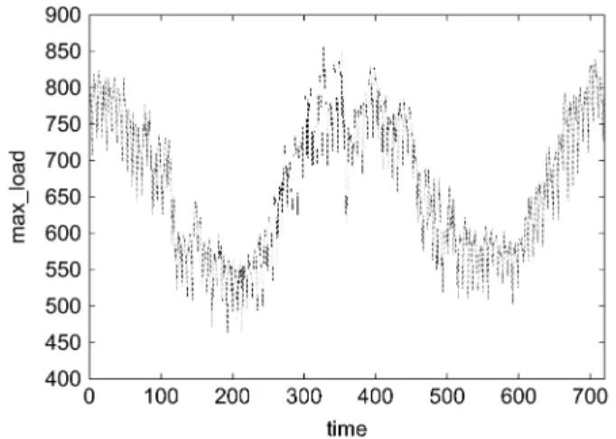
Fig. 1. Maximum daily load.
events, are also investigated. The following observations are somehow specific to the competition, yet they can be applied to general load forecasting.
1) Properties of Load Demand: Load demand data given
are half-hour recorded. Fig. 1 gives a simple description of the maximum daily load demand from 1997 to 1998. By simple analysis, one can easily observe some properties of the load demand. First, the demand has some seasonal patterns: high demand for electricity in the winter while low demand in the summer. This pattern implies the relation between electricity usage and weather conditions in different seasons.
Moreover, if we scrutinize the data further, another load pat-tern could also be observed: a load periodicity exists in every week. Load demand in weekend is usually lower than that of weekdays (Monday through Friday). In addition, electricity de-mand on Saturday is a little higher than that on Sunday.
Further detailed examination of load data, such as daily pat-terns, can also be found, since the data set contains more details (half-hour recorded). However, since the aim of the competi-tion is maximum values of daily load demand, this paper would, without loss of generality, focus on the maximum values only.
2) Climate Influence: In load forecasting, climate
condi-tions have always played an important role. Previous work on short-term load forecasting [1]–[3] also indicate the relation be-tween climate and load demand. Climate conditions considered may include temperature, humidity, illumination, and some special events like typhoon or sleet occurrences. These consid-erations may be regarded on different levels due to different localities. However, while forecasting load demand, more climate information usually give predictions more confidence.
Taking our data for example, as we mentioned earlier, the load data have some seasonal variation, which indicates a great in-fluence of climate conditions. A negative correlation between load demand and daily temperature can be easily observed in Fig. 2. The correlation coefficient between the maximum load and the temperature is . In our data set, it is clear to see that because of the heating use, higher temperature causes lower demands. Yet, unfortunately the only climate information pro-vided in the competition is daily temperature. Such information limitation also affects solutions to such a problem.
There is another interesting observation: the temperature at December 31st, 1998 is the lowest from 1997 to 1998. This
Fig. 2. Correlation between the maximum load and the temperature.
might imply the high uncertainty of the temperature and load of the incoming January 1999, and thus increase the difficulty of the load prediction.
3) Holiday Effects: Local events, including holidays and
festivities, also affect the load demand. These events may lead to higher demand for extra usage of electricity, or otherwise. Influences of these events are usually local and highly depend on the customs of the area. From the two-year load data, it is easy to find out that the load usually lowers down on holidays. With further scrutiny, the load also depends on what holiday it is. On some major holidays such as Christmas or New Year, the demand for electricity may be affected more compared with other holidays.
III. METHODS
SVM is a new and promising technique for data classification and regression [5]. In this section, we briefly introduce support vector regression (SVR) which can be used for time series
pre-diction. Given training data , where are
input vectors and are the associated output value of , the support vector regression solves an optimization problem
(2)
where is mapped to a higher dimensional space by the func-tion is the upper training error ( is the lower) subject to
the -insensitive tube . The
parame-ters which control regression quality are the cost of error , the width of the tube , and the mapping function .
The constraints of (2) imply that we would like to put most
data in the tube . This situation can
be clearly seen from Fig. 3. If is not in the tube, there is an error or which we would like to minimize in the objective function. SVR avoids underfitting and overfitting the training data by minimizing the training error as well as the regularization term . For traditional least-square
where . However, this inner product may be expensive to compute because has too many elements. Hence, we apply “kernel trick” to do the mapping implicitly. That is to employ some special forms which are inner products in higher space yet can be calculated in the original space. Some examples are polynomial kernel
and RBF kernel . They are inner
products in very high dimensional space but can be computed efficiently.
For experiments in this paper, we use the software LIBSVM [6], which is a library for support vector machines, including the implementation of solving (3). While building SVM models, there are some parameters to select. Usually, we conduct cross-validation to choose suitable parameters. Details are in Sec-tion IV-B.
IV. EXPERIMENTS
Though the competition has been closed, the problem still presents an interesting issue in load forecasting. In order to study mid-term load forecasting more, we conduct some experiments on the competition problem. In this section, these experiments and results would be described.
A. Data Preparation
In Section III, we have described the SVM technique. We next need to prepare data sets to build SVM models. For that, we need to encode useful information into the data entries [i.e., in (2)]. In addition, different data encodings affect the selection of modeling schemes. Here we will discuss these issues in detail.
1) Feature Selection: Each component of the training data
is called a feature (attribute). Here, we consider what kind of information should be included. Assuming that is the load of the th day, in general we incorporate information at the same day or earlier as features of . There are a few choices for the feature:
a) Basic Information: Calendar Attributes: In
Sec-tion II-B, we discuss the weekly periodicity of the load demand. Also, as we pointed out earlier, the load demand on holidays is lower than that on nonholidays. Therefore, encoding these information (weekdays and holidays) in the training
mand and temperature have a causal relation in between. In most short-term load forecasting (STLF) works, meteorological in-formation which includes temperature, wind speed, sky cover, etc., has been used to predict the load demand. However, to in-clude the temperature in the training entries, there is one diffi-culty: in this competition, the real temperature data of January 1999 are not provided. In other words, for such mid-term load forecasting, temperature several weeks away are generally not available by weather forecasting. If we would like to encode the temperature in our training entries, we will also need to predict or estimate the temperature of January 1999. Yet, temperature forecast is not easy, especially with such limited data. The use of temperature, therefore, would be a dilemma.
c) Time Series Style or Not: Besides the weekdays,
holi-days and temperature, there is another information we consider to encode as the attributes: the past load demand. That is to intro-duce the concept of time-series into our models. To be more pre-cise, if is the target value for prediction, the vector includes several previous target values as attributes. In the training phase all are known but for future prediction, can be values from previous predictions. For ex-ample, after obtaining an approximate load of January 1, 1999, if , it is used with loads of December 26–31, 1998 for pre-dicting that of January 2. We continue this way until finding an approximate load of January 31. An earlier example using SVR for time series prediction is [8]. As we know, the past load de-mand could affect and imply the future load dede-mand. Therefore, considering to include such information in the models might help forecast the load demand. In fact, in some load forecasting works, time series models have been explored [2], [9].
2) Data Segmentation: Besides the features choices, we
may consider only a subset of load data, since Section II also shows the seasonal pattern. Previous works [1], [2], [7] on load forecasting also propose models built on data of different seasons. This inspires us to do some analyzes for the data segmentation.
Usually, people model time-series data by using the formula-tion
where , and is the embedding
di-mension. However, this formulation is not suitable for a nonsta-tionary time series, because the characteristic of the time series
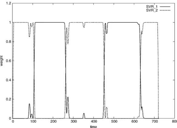
Fig. 4. Unsupervised segmentation for EUNITE data.
may change with time. For such a time series which alternate in time, we can consider a mixture model where
Note that the formulation allows different characteristic func-tions in different time. Given the series , the task is to identify all . We call this unsupervised segmen-tation where earlier work can be found in, for example, [10]. In other words, the method breaks the series into different seg-ments where points in the same segment can be modeled by the same . Recently, [11] states a similar framework using SVR with different parameters tunings. At any time point , these methods consider different weights representing the probability that belongs to corresponding functions. The sum of weight at any given time point is always fixed to one. The weights are iteratively updated until one weight is close to one but others are close to zero. That means eventually is associated to one particular time series.
Now, we can consider the loads as a time series. First, we linearly scale all load data to . Then we can get time series style data by incorporating load of last seven days and weekday information to attributes. After that, we follow the framework of [11] to analyze the data. We consider two possible time series so at each time point there are two weights. The experimental result is in Fig. 4. The x-axis indicates days from January 1997 to December 1998 and the y-axis indicates the weights of two time series. Interestingly, “winter” and “summer” data are automatic separated without any seasonal information. The figure shows that the loads in the summer and in the winter have different characteristics.
Unsupervised data segmentation has been very useful for time series prediction (e.g., [10]). If the training data are associated with different time series, it is better to consider only data seg-ments related to the same series of the last segment. Now the objective of the competition is to predict the load demand of January 1999, so we consider to use only the winter segment for training. Here, we choose January to March and October to December to be our “winter” period, as the analytical result in-dicates. That is, the “winter” data set would contain half of the data in 1997 and 1998. Also, we further extract data of January and February to form another possible training data set. This data set is much smaller than the “winter” one, and it would focus more on the load pattern in the period of our target con-cern.
3) Data Representation: After selecting useful information
and proper data segments for encoding, we can prepare several combinations of training data sets. In these data sets, we encode a training entry [i.e., in (2)] for the particular th day, as fol-lows:
Here we use seven binaries to encode calendar information which includes weekdays, weekends, and holidays, where six are for weekdays and weekends, and the other one for holidays. The six binaries stand for Monday to Saturday respectively and Sunday is represented as all six attributes are set to zero. Also, one numerical attribute is used for normalized temperature data, if the temperature is encoded. As for the past load, if encoded, we use seven numerics for the past seven daily maximum loads. The reason for using “seven” instead of other numbers is the complexity of model selection. We will elaborate more on this
of the other cities close to Slovakia for the estimation. In their report, the temperature for January 1999 was calculated through a linear combination of that of the other three cities. However, for an application in real world, the actual temperature infor-mation of January 1999 at any place is not available since the prediction would be made at December 31, 1998. Therefore, the formulation in [15] might be helpful for inspecting the influence of temperature on the load prediction, yet impractical in use. For experiments here, these two estimations for temperature will be employed in the predicting phase, provided the temperature is encoded in our training data sets.
There is one remark about the testing data of January 1999. In this period, there are two holidays, January 1 and 6. However, in the data entries prepared for the prediction, we remove the holiday flag of these two entries. In other words, we treat them as nonholidays. The reason is that our models cannot learn well about the load demand on holidays. The number of holidays in the training data is too small to provide enough information. Moreover, for the time-series-based approach, inaccurate pre-diction at one day could affect the succeeding forecasting.
B. Implementation and Results
With different schemes of model construction, a series of ex-periments are conducted. MAPE’s of different model schemes are the main concern of our comparison.
Upon the data sets we prepare, SVM models are built for load forecasting. When training an SVM model, there are some parameters to choose. They would influence the performance of an SVM model. Therefore, in order to get a “good” model, these parameters need to be selected properly. Some important ones are:
1) cost of error ;
2) the width of the -insensitive tube; 3) the mapping function ;
4) load of how many previous days included for one training data.
In our experiments, for each training data we simply include the maximum load of the previous seven days. For the parameter , after a few trials we fix it to 0.5. In addition, we consider only the radial basis function (RBF) kernel, as we mention in Section III. The RBF function has the property that
. Note that is a parameter associated with the RBF function which has to be tuned. Thus, parameters left are and
and the search space is reduced.
different characteristics of the data encoding schemes, we em-ploy two procedures for the validation.
For time-series-based approaches, we respectively extract the data entries of January 1997 and 1998 to form the validation set and evaluate the models on them. The performance is decided by averaging the errors of these two validations. As for the non-time-series models, we simply conduct tenfold cross validation to infer the parameters. That is, we randomly divide the training set into ten sets. Using each set as a validation set, we then train a model on the rest. The performance of a model would be the average of the ten validating predictions.
With this procedure, proper and are selected to build a model for the future prediction. We then evaluate its perfor-mance by forecasting the load demand for January 1999. To es-timate the efficiency of model training, we also measure the time consumed to build a model. On a machine with Windows 2000 Professional, CPU 598 MHz, and 256-MB RAM, the time re-quired to train a time-series model ranges from 0.3 to 0.5 s for winter data set and 0.02 s for January-February data. For a non-time-series data set, it takes about 0.15 s to build a model.
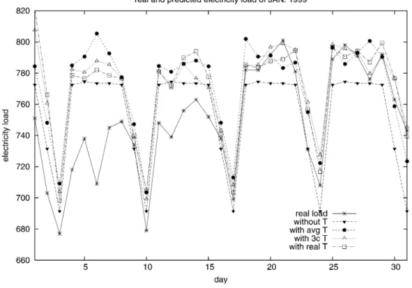
Now we are ready to present experimental results. Table I contains the prediction errors generated by different data encod-ings and segmentations. In the table, the first column shows the data segments used and if the past load demand is encoded. Then the next four columns indicate the predictions with or without the temperature (T): “avg. T” for average temperature, “3c T” for the estimation derived from the three other cities’ data, and “real T” for the real temperature of January 1999.
1) Time-Series Models With Winter Data: In Table I,
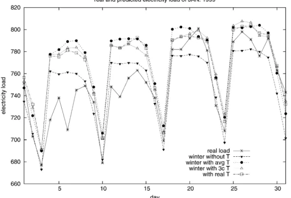
it can be observed that using the “winter” data along with the past loads (time-series information), the model (with ) built without temperature outperforms all others. In fact, the winning entry in the competition is gener-ated by such a model3. The MAPE of using the temperature
of three other cities is smaller than that using the average temperature. Moreover, after the competition is closed, we get the real temperature data of January 1999. We employ the temperature-incorporated models on data sets with the real temperature. The result is shown in the last column of Table I. Its performance, compared with those two using different tem-perature estimations, is not better. That means, even assuming
3During the competition, our validation procedure is different from what we
employ in this paper. Thus, the actual parameters that generate the winning entry is not the same as those we present here. However, the modeling scheme is the same.
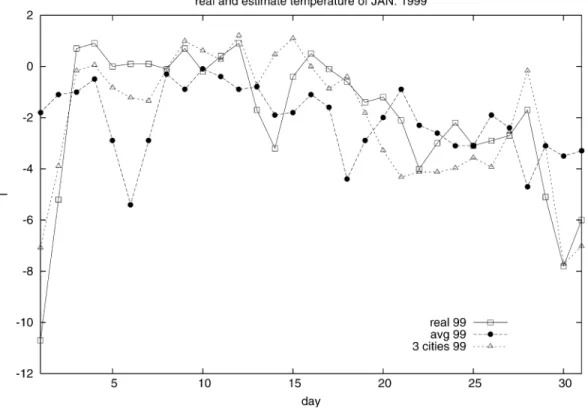
Fig. 5. Estimates and real temperature in Jan. 1999.
the real temperature is known, the forecasting result is still not satisfactory.
2) Time-Series Models With January-February Data: With
the training set containing only data of January and February, the model built without temperature also performs better than all others built with temperature. This is the same as using the “winter” data segment.
3) Non-Time-Series Models With Winter Data: Besides
time-series-based approaches, we build models without taking the past load demand as attributes. The training set of these models is limited to the “winter” segment. In Table I, we show the test errors of the forecast with or without temperature information. Just like the aforementioned experimental results, the MAPE of prediction on the data set without temperature is better than that with. Actually as one can see in Fig. 8, the forecast generated by the model using only calendar attributes is the same weekly. That is because besides the calendar at-tributes, the data set does not provide any other information for the model.
4) Remarks: From the results, an interesting observation
can be made: models built without the temperature generally perform better than those built with. This renders the issue about the usage of temperature information. As we mentioned earlier, temperature information is important for load forecasting. However, models constructed with such information may be really sensitive to the temperature and thus the estimation for the temperature in 1999 would surely affect the performance of the models.
In Fig. 5, the real temperature data and the two estimations are shown. Figs. 6–8 plot the predicted values as well as the real load demand of January 1999. Roughly the higher the tempera-ture is, the lower the demand is. Interestingly, the model using real temperature cannot predict the load demand more precisely
than using the estimation coming from the data of the three other cities. This result somehow implies the difficulty of incorpora-tion of the temperature. To further inspect the influence of tem-perature information, we also conduct some simple experiments with another part of the data set. Targeting at predicting the loads in August 1998, we use another period of the data to build two different time-series models, one with temperature and the other without. The resulting MAPEs are both 2.47%. Note that for the temperature-included model, we already use the real tem-perature of August 1998, which, again, is not available for prac-tical use. This confirms the futility of temperature information in such a mid-term load forecasting problem. In fact, as we com-pute the correlation coefficient between the maximum load and the temperature for each month instead of the whole two year, we find they are variant (ranging from to 0.32). This also indicates the fuzzy correlation between the load and the temper-ature in a shorter period.
Models built on data segments of January and February per-form not as well as those built on the “winter” segments. We think the main reason is that, with the limited data given (only two years), such data segments cannot provide enough informa-tion for models compared with the “winter” segments that con-tains more entries. Therefore, though data set containing data only from January and February may represent the period of the prediction better, due to the limited data, models built on such segments are somehow not as competitive as those built with more information.
For comparison, models without time-series information are also built. The performance of such models is less competitive. This shows that models built without the past loads may not be able to learn the tendency of the load demand. Moreover, if the temperature is used to build the model, it would be the main attribute that affects the predicted values. Due to the limited data
Fig. 6. Estimates and real electricity load in January 1999, with “winter” data.
Fig. 7. Estimates and real electricity load in January 1999, with January-February data.
and the fuzzy correlation between the temperature and the load demand, such incorporation of temperature information could introduce higher variance into the model and result in unreliable prediction. That is why even using the real temperature, the error is higher than that of using only calendar information.
Recall that the temperature of the last day in 1998 is the lowest of the whole data set, but the load is not extremely high.
More-over, the correlation coefficient between the load and the tem-perature in December 1998 is 0.092. All these could make the forecast difficult for temperature-related models; however, with the time-series information, the models could at least catch the load tendency, and thus give reasonable predictions following the trend of December 1998. That is why here the time-series-based models perform better than nontime-series-time-series-based ones.
Fig. 8. Estimates and real electricity load in January 1999, with nontime-series model.
V. DISCUSSIONS ANDCONCLUSIONS
A. Comparisons
1) With Local Models: Besides SVM, during the
competi-tion we also tried another method, local models. Local modeling is a simple analysis scheme for time-series data. With stationary time-series data, local models can also have good performance [16]. They generate predictions by finding segments of the time series that closely resemble the segment of the points immedi-ately proceeding the point to be predicted. Then the prediction is usually the average of elements that occurred immediately after these similar segments of points.
Practically we have to decide the length of each segment and the number of similar segments. Here we simply take loads of seven days as a segment and select the closest segment. That is, if we would like to predict the load on date , we compute the
distances between segment and other
segments , for . After
finding the closest segment with , we use the load as the prediction. In addition, we take the information of weekdays into consideration since there is a weekly pattern in the load demand. That means we choose the closest segment with so that the weekdays of date and are the same. Then, we take the load on date , as the predicted value.
Using the local-model scheme described above, we tried to forecast the load in January 1999. However, the result is not promising. The MAPE of the predictions is 8.81%. Actually, some competitor [17] also used local models to do the forecast.
2) With Neural Network Models: Among competitors,
neural network models are quite popularly employed. Here we also employ the technique to conduct comparisons.
The implementation of neural network we choose to work with is nnet, which is wrapped in the package VR [18] for the statistical computing environment R [19]. There are also several tunable parameters while training a neural network, such as decay rate for weight, number of units in the hidden
layer, and etc. Hence in our experiments, we try to tune
these parameters along with the two data sets of winter, with or without temperature. The determination for the values of parameters is similar to what we used for SVM models. Different values for parameters are used to build models and then validate on data sets of Januaries in 1997 and 1998. With the chosen parameters we finally train models and use them to forecast loads in January 1999.
The models with tuned parameters, however, do not perform well on the problem. Using temperature information, the built model predicts the loads of January 1999 with MAPE reaching to 5.73%, while the model without temperature produces results with 7.8% for the error metric. Generally, the neural networks we tune here do not perform well. There is one extreme case that the tuned model generates a single value for all the prediction with a MAPE of 3.79%. That single value, in a way, is a kind of average the model predicts for this problem. Considering the difficulties of parameter selection and insufficient proficiency in neural networks, we then decide to simply use the default values to train our models. Surprisingly, the results generated by these models are better. The MAPE is 3.63% for the data set with temperature and 4.94% for that without.
Overall, the results produced by neural networks are not satisfactory at all. However, these results indicate more about the incapability of the neural networks due to the difficulty of choosing parameters.
between temperature and load demand is most used. Many com-petitors use the temperature, along with some other informa-tion, to build causal models while some also incorporate with time-series analysis (e.g., [22], [24] and [17]). The techniques competitors used for causal models include neural networks ([21], [13], [25] and [14]), adaptive logic network [12], fuzzy rule-based models [26], self-organizing maps combined with ARIMA models [27], clustering [28], etc. However, the use of causal relation between temperature and load demand, would involve the inference for the temperature of January 1999.
In fact, some competitors do try to predict or infer the weather condition of January 1999 ([29], [21] and [15]), yet, with the limited data, forecasting the temperature may even be a more difficult problem. Without good forecast for the temperature, the model might end up with imprecise prediction, even though it may perform well in the training phase.
Holiday is another issue. For most competitors, load fore-casting on holidays is not easy to handle. The difficulty is that the historical load data on holidays are not enough, and thus make the behavior of load demand on these special days hard to model. In our work, we do include holiday information in the training phase. However, while predicting the load in 1999, we remove the holiday flags on January 1 and 6. Other competitors treat some holidays as Saturday or Sunday [21], [12], build an-other model for holidays [13], or manually adjust the predicted result [22].
B. Conclusion
Among these different proposed solutions, we find that choosing appropriate data segments seems to enhance the model performance. Furthermore, models built with continuous estimation of the future temperature, may be inaccurate in the end. In other words, including unprecise information causes higher variance on prediction so a conservative approach using only available correct information is sometimes recommended for such mid-term load forecasting. We have also demonstrated a validation procedure to judge whether temperature should be incorporated or not. As the experimental results show, the introduction of the time-series attributes also gives models better information to forecast load demand more precisely. Ac-tually, these considerations are what we were upon to propose the time-series based, winter-data only, without temperature information, model which generated the winning entry.
tomated load forecasting assistant,” IEEE Trans. Power Syst., vol. 3, pp. 908–914, Aug. 1988.
[4] C. Cortes and V. Vapnik, “Support-vector network,” Mach. Learn., vol. 20, pp. 273–297, 1995.
[5] V. Vapnik, Statistical Learning Theory. New York: Wiley, 1998. [6] C.-C. Chang and C.-J. Lin. (2001) LIBSVM: A
Li-brary for Support Vector Machines. [Online]. Available: http://www.csie.ntu.edu.tw/~cjlin/libsvm
[7] S. Rahman and O. Hazim, “A generalized knowledge-based short-term load-forecasting technique,” IEEE Trans. Power Syst., vol. 8, pp. 508–514, May 1993.
[8] K.-R. Müller, A. Smola, G. Rätsch, B. Schölkopf, J. Kohlmorgen, and V. Vapnik, “Predicting time series with support vector machines,” in
Ad-vances in Kernel Methods—Support Vector Learning, B. Schölkopf, C.
J. C. Burges, and A. J. Smola, Eds. Cambridge, MA: MIT Press, 1999, pp. 243–254.
[9] N. Amjady, “Short-term hourly load forecasting using time-series mod-eling with peak load estimation capability,” IEEE Trans. Power Syst., vol. 16, pp. 498–505, Aug. 2001.
[10] K. Pawelzik, J. Kohlmorgen, and K.-R. Müller. (1996) Annealed com-petition of experts for a segmentation and classification of switching dynamics. Neural Computation. [Online]. Available: http://cite-seer.nj.nec.com/pawelzik96annealed.html
[11] M.-W. Chang, C.-J. Lin, and R. C. Weng, “Analysis of switching dy-namics with competing support vector machines,” in Proc. IJCNN, 2002, pp. 2387–2392.
[12] D. Esp, “Adaptive logic networks for east slovakian electrical load fore-casting,” in Electricity Load Forcast Using Intelligent Technologies, P. Sinˇcák, J. Strackeljan, M. Kolcun, D. Novotný, and P. Szathmáry, Eds: EUNITE: The European Network on Intelligent Technologies for Smart Adaptive Systems, 2002, pp. 55–74.
[13] E. Castillo, B. Guijarro, and A. Alonso, “Electricity load forecast using functional networks,” in Electricity Load Forcast Using Intelligent
Tech-nologies, P. Sinˇcák, J. Strackeljan, M. Kolcun, D. Novolný, and P.
Sza-thmáry, Eds: EUNITE: The European Network on Intelligent Technolo-gies for Smart Adaptive Systems, 2002, pp. 75–84.
[14] I. King and J. Tindle, “Storage of half hourly electric metering data and forecasting with artificial neural network technology,” in Electricity
Load Forcast Using Intelligent Technologies, P. Sinˇcák, J. Strackeljan,
M. Kolcun, D. Novotný, and P. Szathmáry, Eds: EUNITE: The Euro-pean Network on Intelligent Technologies for Smart Adaptive Systems, 2002, pp. 93–106.
[15] W. Kowalczyk, “Averaging and data enrichment: Two approaches to electricity load forecasting,” in Electricity Load Forcast Using
Intelli-gent Technologies, P. Sinˇcák, J. Strackeljan, M. Kolcun, D. Novotný,
and P. Szathmáry, Eds: EUNITE: The European Network on Intelligent Technologies for Smart Adaptive Systems, 2002, pp. 209–218. [16] J. McNames, J. A. K. Suykens, and J. Vandewalle, “Winning entry of the
K. U. leuven time series prediction competition,” Int. J. Bifurc. Chaos, vol. 9, no. 8, pp. 1485–1500, 1999.
[17] G. Bontempi, “Eunite world-wide competition: Research report,” in
Electricity Load Forcast Using Intelligent Technologies, P. Sinˇcák, J.
Strackeljan, M. Kolcun, D. Novotný, and P. Szathmáry, Eds: EUNITE: The European Network on Intelligent Technologies for Smart Adaptive Systems, 2002, pp. 33–40.
[18] W. N. Venables and B. D. Ripley, Modern Applied Statistics with S, 4th ed. New York: Springer-Verlag, 2002.
[19] R Development Core Team, R Foundation for Statistical Computing. (2003) R: A Language and Environment for Statistical Computing, Vi-enna, Austria. [Online]. Available: http://www.R-project.org
[20] P. Sinˇcák, J. Strackeljan, M. Kolcun, D. Novotný, and P. Szathmáry, Eds., Electricity Load Forcast Using Intelligent Technologies: EUNITE: The European Network on Intelligent Technologies for Smart Adaptive Systems, 2002.
[21] A. Lewandowski, F. Sandner, and P. Protzel, “Prediction of electricity load by modeling the temperature dependencies,” in Electricity Load
Forcast Using Intelligent Technologies, P. Sinˇcák, J. Strackeljan, M.
Kolcun, D. Novotný, and P. Szathmáry, Eds: EUNITE: The European Network on Intelligent Technologies for Smart Adaptive Systems, 2002, pp. 107–114.
[22] E. Pelikán, “Middle-term electrical load forecasting by time series de-composition,” in Electricity Load Forcast Using Intelligent
Technolo-gies, P. Sinˇcák, J. Strackeljan, M. Kolcun, D. Novotný, and P. Szathmáry,
Eds: EUNITE: The European Network on Intelligent Technologies for Smart Adaptive Systems, 2002, pp. 167–176.
[23] W. Brockmann and S. Kuthe, “Different models to forecast electricity loads,” in Electricity Load Forcast Using Intelligent Technologies, P. Sinˇcák, J. Strackeljan, M. Kolcun, D. Novotný, and P. Szathmáry, Eds: EUNITE: The European Network on Intelligent Technologies for Smart Adaptive Systems, 2002, pp. 41–54.
[24] F. Rivieccio, “SVM for an electricity load forecast problem,” in
Elec-tricity Load Forcast Using Intelligent Technologies, P. Sinˇcák, J.
Strack-eljan, M. Kolcun, D. Novotný, and P. Szathmáry, Eds: EUNITE: The European Network on Intelligent Technologies for Smart Adaptive Sys-tems, 2002, pp. 177–186.
[25] D. Živˇcák, “Electricity load forecasting using ANN,” in Electricity Load
Forcast Using Intelligent Technologies, P. Sinˇcák, J. Strackeljan, M.
Kolcun, D. Novotný, and P. Szathmáry, Eds: EUNITE: The European Network on Intelligent Technologies for Smart Adaptive Systems, 2002, pp. 219–231.
[26] R. C. Weizenegger, “Maximum electricity load problem,” in Electricity
Load Forcast Using Intelligent Technologies, P. Sinˇcák, J. Strackeljan,
M. Kolcun, D. Novotný, and P. Szathmáry, Eds: EUNITE: The European Network on Intelligent Technologies for Smart Adaptive Systems, 2002, pp. 187–208.
[27] G. A. Ivakhnenko, “Inductive self-organizing algorithm for maximum electrical load prediction,” in Electricity Load Forcast Using Intelligent
Technologies, P. Sinˇcák, J. Strackeljan, M. Kolcun, D. Novotný, and P.
Szathmáry, Eds: EUNITE: The European Network on Intelligent Tech-nologies for Smart Adaptive Systems, 2002, pp. 85–92.
[28] Z. Boger. (2001) Electricity Load Forecast Using Artificial Neural Networks Clustering. [Online]. Available: http://neuron.tuke.sk/compe-tition/
[29] A. Lotfi, “Application of learning fuzzy inference systems in electricity load forecast,” in Electricity Load Forcast Using Intelligent
Technolo-gies, P. Sinˇcák, J. Strackeljan, M. Kolcun, D. Novotný, and P. Szathmáry,
Eds: EUNITE: The European Network on Intelligent Technologies for Smart Adaptive Systems, 2002, pp. 123–130.
Bo-Juen Chen received the B.S. degree in computer science and information engineering in 2001 and the M.S. degree in computer science and information en-gineering in 2003, both from National Taiwan Uni-versity, Taipei, Taiwan, R.O.C.
His research interests include data mining, ma-chine learning, and related applications.
Ming-Wei Chang received the B.S. degree in 2001 and the M.S. degree in 2003, both in computer science and information engineering, from National Taiwan University, Taipei, Taiwan, R.O.C..
His research interests include machine learning, numerical optimization, and algorithm analysis.
Chih-Jen Lin (S’91–M’98) received the B.S. degree in mathematics from National Taiwan University, Taipei, Taiwan, R.O.C., in 1993 and the M.S. and Ph.D. degrees from the Department of Industrial and Operations Engineering, University of Michigan, Ann Arbor, in 1998.
He is currently an Associate Professor in the De-partment of Computer Science and Information En-gineering, National Taiwan University. His research interests include machine learning, numerical opti-mization, and applications of operations research.