Exact Computation of Median Surfaces Using
Optimal 3D Graph Search
Zhengwang Wu1, Xiaoyi Jiang2, Nanning Zheng1, Yuehu Liu1, Dachuan Cheng3 1
Institute of Artificial Intelligence and Robotics, Xi’an Jiaotong University, China
2Department of Mathematics and Computer Science, University of M¨unster, Germany 3
Department of Biomedical Imaging, China Medical University, Taiwan
Abstract. In this paper we formulate the generalized median surface problem and present its exact solution by means of an optimal 3D graph search algorithm. In addition to the general interest in median surface computation our work is also motivated by the task of parameter space exploration without ground truth, which is an effective means of dealing with the difficult parameter problem. A concrete application in this con-text will be demonstrated on artery boundary detection in ultrasound data. It will be shown that the median computation can not only avoid the parameter training, but also potentially achieve even better results than with trained parameters. Particularly in situations with no available ground truth, the median-based approach can thus be a good alternate.
1
Introduction
Median computation has turned out to be a useful concept in pattern recogni-tion [1]. Given an object set S in space U , the generalized median is defined by x ∈ U which minimizes the sum of distances to all objects in S and can be considered as a good representative of the given set. Another motivation of median computation is to eliminate some erroneous objects by averaging over all objects. Generally, the median concept is motivated by well established re-sults from supervised classifier combination: By averaging the rere-sults of several classifiers a more reliable classification can be achieved [2].
The median concept has been concretized to a lot of domains including vec-tors [3], strings [4], graphs [5], clusterings [6], and segmentations [7]. In [8] the 2D contour median problem is investigated. In this work we consider the related 3D surface median problem.
There exist only very few general frameworks for median computation. One such framework described in [5] is based on an embedding into the vector s-pace. The median vector is computed by means of the Weiszfeld algorithm [3] and inversely transformed to the original space. Another general framework [9] computes the weighted mean of a pair of objects in an evolutionary scheme.
1
Both frameworks are approximative only and therefore suitable for those medi-an problems with inherently high computational complexity. Indeed, they have been applied to computing generalized median of strings [4, 9] and graphs [5], both being of N P-hard problems.
Many median computation algorithms have been developed for specific do-mains to integrate as much as possible domain-specific knowledge in order to obtain possibly exact solutions in an efficient way. For instance, the general-ized median string problem is N P-hard for the edit distance, but simplified histogram-based distances enable low-order polynomial time [10]. For 2D tours dynamic programming can be used to determine the optimal median con-tour in a time linear to the image size [8]. In this work we will show that for the class of so-called terrain-like surfaces (to be formally defined later) consid-ered here, we can apply an optimal 3D graph search algorithm to exactly and efficiently solve median surface problem.
In addition to the general interest in median surface computation this work is also motivated by our recent work on exploring the parameter space of segmen-tation algorithms without ground truth. Ensemble techniques similar to multiple classifier systems should be developed to achieve the best possible segmentation result on a per-image basis.
The outline of this paper is as follows. In Section 2 we define the median surface problem under consideration, which is further motivated by segmentation parameter exploration in Section 3. The median surface problem will be exactly solved by applying an optimal 3D graph search algorithm (Section 4). We report experimental results to demonstrate the usability of median surface computation in the context of segmentation parameter exploration in Section 5. Finally, some discussions in Section 6 conclude the paper.
2
Median Surface Problem
The surfaces of concern in this paper are terrain-like (height-field) as specified in Definition 1.
Definition 1. A terrain-like surface is a function: f : X × Y → Z with X = {1, 2, . . . , M }, Y = {1, 2, . . . , N }, and Z = {1, 2, . . . , L}. In order to guarantee surface connectivity in 3D, an additional smoothness constraint requires |f (x + 1, y) − f (x, y)| ≤ ∆xand |f (x, y + 1) − f (x, y)| ≤ ∆y for small positive constants
∆xand ∆y.
In the following we will use the term ”surface” only for the sake of simplicity. This class of surfaces are very common in image analysis. In 3D biomedical volume datasets an important task is to detect such terrain-like surfaces, possibly in an optimal manner. Stacking 2D images along the time axis also results in 3D volume datasets and related terrain-like surface detection tasks.
Given a set S of K surfaces {S1, S2, . . . , SK} and a distance function d()
defined by: S = arg min s∈US K X i=1 d(s, Si) (1)
where US represents the space (universe) of all potential solutions, i.e. surfaces
within the volume X × Y × Z.
The distance function is defined by:
d(s, Si) = M X x=1 N X y=1 wxy· ρ(s(x, y), Si(x, y)) (2)
where ρ is a dissimilarity function for scalar values. Any function suitable for a certain application, e.g. Lp, can be used for this purpose. In particular, those
from robust statistics [11] may help to achieve improved performance against outliers in the input surface data. In the simplest case the weight wxy can be
set to be constant for all (x, y) positions. But in general, a location-sensitive weight gives us more flexibility to incorporate application-specific knowledge to a largest extent. For our segmentation parameter exploration we will fully utilize this flexibility.
3
Motivation
One motivation of median surface computation is exploring segmentation pa-rameter space without ground truth. Segmentation algorithms mostly have some parameters and their optimal setting is not a trivial task. In automatic param-eter training a training image set with (manual) ground truth segmentation is assumed to be available. Then, a subspace of the parameter space is explored to find out the best parameter setting. For each parameter setting candidate a performance measure is computed in the following way:
– Segment each image of the training set based on the parameter setting; – Compute a performance measure by comparing the segmentation result and
the corresponding ground truth;
– Compute the average performance measure over all images of the training set.
The optimal parameter setting is given by the one with the largest average per-formance measure. Since fully exploring the subspace can be very costly, space subsampling [12] and genetic search [13] have been proposed. While this ap-proach is reasonable and has been successfully practiced in several applications, its fundamental disadvantage is the need of ground truth segmentation. The manual generation of ground truth is always painful and thus a main barrier of wide use in many situations.
Recently, it is proposed to apply the concept of generalized median for im-plicitly exploring the parameter space without the need of ground truth segmen-tation. Assuming a reasonable subspace of the parameter space (i.e. a lower and
upper bound for each parameter), it is sampled into a finite number M of param-eter settings. Then, the segmentation procedure is run for all the M paramparam-eter settings and the generalized median of the M segmentation results is computed. The rationale here is that the median segmentation tends to be a good one with-in the explored parameter subspace, as successfully demonstrated for 2D contour detection [8] and region segmentation [7]. Segmentation of terrain-like surfaces is one of the most important problems in (biomedical) image analysis. Thus, median surface computation can help to alleviate the segmentation parameter problem in 3D surface segmentation as well.
Another situation is segmentation of 2D images along the time axis. Many algorithms from the literature, e.g. [14], perform the segmentation independently on all images and thus cannot guarantee a continuous segmentation over time, which is highly desired when working with high-speed imaging devices. If the parameter space exploration technique described above is applied in this case to the 3D volumes by stacking all image-wise segmentations along the time axis, we obtain a continuous temporal segmentation without any extra effort as a nice spinoff of handling the parameter problem. For doing this, we certainly need to relax the input for the median surface computation to potentially include discontinuous surfaces. But this is not a problem at all.
In summary median surface computation is not only an interesting topic in its own right but also of substantial practical value. This motivates us to find an efficient way for exact median surface computation.
4
Exact computation by optimal 3D graph search
In this section we show that the median surface problem defined in Eq. (1) can be transformed into an optimal 3D surface detection problem, which is solvable by an optimal 3D graph search algorithm in low-order polynomial time.
First, we reformulate Eq. (1) as follows.
S = arg min s∈US K X i=1 d(s, Si) = arg min s∈US K X i=1 M X x=1 N X y=1 wxy· ρ(s(x, y), Si(x, y)) = arg min s∈US M X x=1 N X y=1 wxy· K X i=1 ρ(z = s(x, y), Si(x, y)) | {z } cxyz = arg min s∈US M X x=1 N X y=1 cxyz | {z } C(s) = arg min s∈US C(s) (3)
A candidate solution surface s ∈ US is characterized by the z-value s(x, y) for
each position (x, y) on the grid X ×Y . We assign each point (x, y, z) in the volume X × Y × Z a cost cxyz, which is determined by its deviations (in z-direction)
from the K input surfaces Si(x, y) and the position-specific weight wxy. Then,
the goodness of a candidate solution surface s can be measured by C(s), i.e. summing up the costs of all positions. Therefore, the median surface is simply the optimal surface with minimal cost from the solution space US (consisting of
all terrain-like surfaces within the volume X × Y × Z).
The discussion above leads to the following new optimization problem. We first compute a cost cxyzfor each point (x, y, z) in the volume X × Y × Z. Then,
the median surface is determined by finding the terrain-like surface within the volume with the minimal sum of costs.
It is important to notice that we cannot solve this optimization problem by computing the optimal z-value for each of the M × N positions (x, y) indepen-dently, which could be done, for instance, by enumerating all z-values out of Z and minimizing cxyz. Doing it this way, we may encounter the trouble of
generat-ing a discontinuous resultant surface. Only for simple cases (e.g. constant weight wxy and ρ = L2) the simple position-wise optimization is guaranteed to deliver
an optimal continuous resultant surface. But in general, a global optimization approach is needed.
For the special case N = 1 (i.e. the y-axis vanishes), the 3D optimal sur-face segmentation is reduced to a 2D optimal contour detection problem. This simplified problem was solved in [8] by a highly efficient dynamic programming algorithm. Unfortunately, there is no direct way of extending the dynamic pro-gramming solution to the 3D problem at hand.
Fortunately, the optimal 3D graph search algorithm described in [15] solves exactly our 3D optimal surface detection problem. In the following we briefly present the most important steps of this algorithm and the readers are referred to [15] for more details. A node-weighted directed graph G = (V, E, W ) is con-structed as follows. For each point (x, y, z) in the volume X × Y × Z a corre-sponding node V (x, y, z) is defined in G, whose weight W (x, y, z) is assigned according to: W (x, y, z) = ( cxyz− cxy,z−1 z > 1 cxyz z = 1 (4)
where cxyz is the cost defined in Eq. (3). G contains two types of arcs: E =
Ea ∪ Er. The set Ea of intraposition arcs rules the connections within the
same position (x, y). Each node V (x, y, z) (z > 1) has a direct arc to the n-ode V (x, y, z − 1) below it, i.e.,
The set Er of interposition arcs rules the connections of adjacent positions and is defined by: Er = {< V (x, y, z), V (x + 1, y, max(0, z − ∆x)) > | x ∈ {1, . . . , M − 1}, z ∈ Z} ∪ {< V (x, y, z), V (x − 1, y, max(0, z − ∆x)) > | x ∈ {2, . . . , M }, z ∈ Z} ∪ {< V (x, y, z), V (x, y + 1, max(0, z − ∆y)) > | y ∈ {1, . . . , N − 1}, z ∈ Z} ∪ {< V (x, y, z), V (x, y − 1, max(0, z − ∆y)) > | y ∈ {2, . . . , N }, z ∈ Z}
Given the constructed digraph G, a closed set C is a subset of nodes such that all successors of any nodes in C are also contained in C. The cost of a closed set is the total cost of all its nodes. In [15] it was shown that the original optimal surface detection problem is equivalent to finding a minimum nonempty closed set in G. This is a well studied problem in graph theory and can be solved by computing a minimum s−t cut in a related graph Gst (see [15] for the details
of constructing Gst from G). In our implementation the Boykov-Kolmogorov
algorithm [16] is applied to compute the minimum s−t cut. For a graph with n nodes and m arcs, the theoretical worst-case time complexity for this algorithm is O(n2mc), where c is the cost of the minimum cut.
5
Experimental results
In this section we demonstrate a practical use of median surface computation by applying the algorithm described above to segmentation parameter exploration on ultrasound data.
5.1 Ultrasound image data and experimental settings
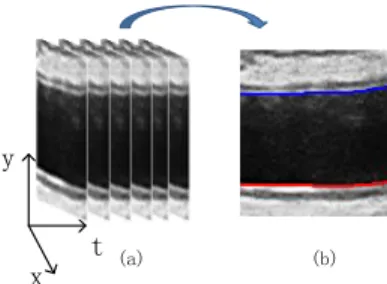
The task considered here is the extraction of artery boundaries from ultrasound videos. An artery has a near wall and a far wall, as illustrated in Fig. 1(b). Along with the time axis the 2D images can be regarded a 3D volume, see Fig. 1(a). Three ultrasound videos from patients were used in our experiments. For these videos, a ground truth of the arterial walls (golden standard) was labeled manually.
The algorithm from [14] was applied to detect the two contours in each 2D image. These contours are stacked to build 3D, possibly discontinuous, surfaces. For each video, 100 different parameter settings were used to generate 100 near wall surfaces and 100 far wall surfaces. Then, a median surface was computed from each of the two surface ensembles. For this computation a position-wise weight wxy, see Eq. (2), is needed to measure the dissimilarity between the
x y
t (a) (b)
Fig. 1. Ultrasound video. (a) Along with the time axis the 2D images build a 3D volume. (b) The near (blue) and far (red) wall of the artery in a single image.
implementation this was done in the following way. A normal distribution is estimated using all z-values of the 100 input surfaces at (x, y). Then, wxy is
chosen to be [1.0 - density at z = s(x, y)].
For comparison purpose the best-performing one among the 100 parameter settings was determined for each video by comparing with the ground truth. In all our tests the comparison between two surfaces, e.g. a segmented surface and a ground truth, was done by computing the average L1deviation in z per (x, y)
position.
5.2 Comparison with the best parameter setting
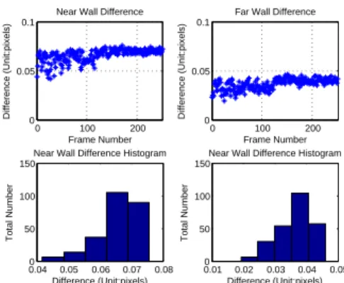
Totally we have 6 test cases (near and far wall, 3 videos). For each of the test cases the median surface was computed from the 100 input surfaces and compared with the surface from the best-performing parameter setting, which was determined by a per-video basis. The results are shown in Table 1, which are further detailed in Figures 2-4 with the average deviation per image and the distribution of deviations.
These results indicate that basically no real performance differences exist between the best-performing parameter setting and our approach of parameter space exploration by means of median surface computation. This fact is particu-larly remarkable since the parameter optimization was done on a per-video basis in contrast to the popular practice of using training images. In the latter case the trained best parameters can be expected to achieve good results on addi-tional test images, but in general not the best result per image. Overall, it can be concluded that without using any ground truth information, the generalized median technique is able to produce segmentations of identical quality as the training approach.
5.3 Comparison with the ground truth
Since all the real data include manually labeled ground truth (GT), we com-pared our median result with the ground truth. The average L1deviation in z is
0 100 200 0
0.05 0.1
Near Wall Difference
Frame Number Difference (Unit:pixels) 0 100 200 0 0.05 0.1
Far Wall Difference
Frame Number Difference (Unit:pixels) 0.040 0.05 0.06 0.07 0.08 50 100 150
Near Wall Difference Histogram
Difference (Unit:pixels) Total Number 0.01 0.02 0.03 0.04 0.05 0 50 100 150
Near Wall Difference Histogram
Difference (Unit:pixels)
Total Number
Fig. 2. Comparison with the best parameter setting: video 1.
0 20 40 60 80 0
0.05 0.1
Near Wall Difference
Frame Number Difference (Unit:pixels) 0 20 40 60 80 0 0.05 0.1
Far Wall Difference
Frame Number Difference (Unit:pixels) 0.020 0.04 0.06 0.08 10 20 30 40
Near Wall Difference Histogram
Difference (Unit:pixels) Total Number 0.01 0.02 0.03 0.04 0.05 0 10 20 30
Near Wall Difference Histogram
Difference (Unit:pixels)
Total Number
Fig. 3. Comparison with the best parameter setting: video 2.
0 50 100
0 0.05 0.1
Near Wall Difference
Frame Number Difference (Unit:pixels) 0 50 100 0 0.05 0.1
Far Wall Difference
Frame Number Difference (Unit:pixels) 0.040 0.05 0.06 0.07 0.08 20 40 60
Near Wall Difference Histogram
Difference (Unit:pixels) Total Number 0.02 0.03 0.04 0.05 0 10 20 30 40
Near Wall Difference Histogram
Difference (Unit:pixels)
Total Number
Fig. 4. Comparison with the best parameter setting: video 3.
video #images near wall far wall 1 251 0.066 0.036
2 86 0.063 0.034
3 111 0.065 0.036
Table 1. Comparison with the best parameter setting (unit: pixels).
video #images comparison type near wall far wall median vs. GT 0.341 0.336 1 251 BP vs. GT 0.492 0.388 median vs. GT 0.321 0.365 2 86 BP vs. GT 0.504 0.478 median vs. GT 0.312 0.334 3 111 BP vs. GT 0.481 0.436
Table 2. Comparison with the ground truth GT (unit: pixels).
setting (BP) were also compared with GT. Some results are given in Figure 5 for illustration purpose. As can be seen in Table 2, these results turn out to be inferior to our median segmentation results. Using our median surface algorith-m thus can not only avoid the paraalgorith-meter training (which is only possible with existing ground truth), but also potentially achieve even better segmentation results than with the best parameters. This fact is clearly due to the ensemble nature of the median surface computation.
6
Conclusion
In this paper we have formulated the generalized median surface problem and presented its exact solution by means of an optimal 3D graph search algorithm. This work is motivated by the task of parameter space exploration without ground truth, which is an effective means of dealing with the difficult parameter problem and has been successfully applied to domains like 2D contour detection [8] and region segmentation [7]. Our median surface computation algorithm thus provides a useful tool for parameter exploration in 3D surface segmentation or 2D contour segmentation in a temporal context. A concrete application has been demonstrated on artery boundary detection in ultrasound data, which confirmed the findings from the previous studies. That is, the median computation can not only avoid the parameter training, but also potentially achieve even better results than with trained parameters. Parameter training is only possible with existing ground truth, which is not always available. The median-based approach can thus be a good alternate in case of no ground truth.
The optimal 3D graph search algorithm in [15] designed for terrain-like sur-face detection has several interesting extensions. One extension is for
simultane-ously detecting multiple surfaces subject to certain spatial constraints. In addi-tion, the algorithm can be applied to tube-like, or more generally star-shaped, surface segmentation based on transforming the initial image data to another space. These extensions allow us to study the median surface problem for a broader range of surface classes and will be investigated in future.
References
1. Jiang, X., Bunke, H.: Learning by generalized median concept. In: Pattern Recog-nition and Machine Vision. River Publishers (2010) 1–16
2. Rokach, L.: Pattern Classification Using Ensemble Methods. World Scientific (2010)
3. Weiszfeld, E., Plastria, F.: On the point for which the sum of the distances to n given points is minimum. Annals of Operations Research 167 (2009) 7–41 4. Jiang, X., Wentker, J., Ferrer, M.: Generalized median string computation by
means of string embedding in vector spaces. Pattern Recognition Letters 33 (2012) 842–852
5. Ferrer, M., Karatzas, D., Valveny, E., Bardaj´ı, I., Bunke, H.: A generic frame-work for median graph computation based on a recursive embedding approach. Computer Vision and Image Understanding 115 (2011) 919–928
6. S.Vega-Pons, J.Ruiz-Shulcloper: A survey of clustering ensemble algorithms. Int. Journal of Pattern Recognition and Artificial Intelligence 25 (2011) 337–372 7. Franek, L., Abdala, D.D., Vega-Pons, S., Jiang, X.: Image segmentation fusion
using general ensemble clustering methods. In: Proc. of Asian Conf. on Computer Vision. Volume 4. (2010) 373–384
8. Wattuya, P., Jiang, X.: A class of generalized median contour problem with exact solution. In: Proc. of SSPR/SPR. (2006) 109–117
9. Franek, L., Jiang, X.: Evolutionary weighted mean based framework for generalized median computation with application to strings. In: Proc. of SSPR/SPR. (2012) 70–78
10. Solnon, C., Jolion, J.M.: Generalized vs set median strings for histogram-based distances: Algorithms and classification results in the image domain. In: Proc. of GbR. (2007) 404–414
11. Stewart, C.: Robust parameter estimation in computer vision. SIAM Reviews 41 (1999) 513–537
12. Min, J., Powell, M.W., Bowyer, K.W.: Automated performance evaluation of range image segmentation algorithms. IEEE Transactions on Systems, Man, and Cyber-netics, Part B 34 (2004) 263–271
13. Pignalberi, G., Cucchiara, R., Cinque, L., Levialdi, S.: Tuning range image seg-mentation by genetic algorithm. EURASIP J. Adv. Sig. Proc. 2003 (2003) 780–790 14. Cheng, D., Jiang, X.: Detections of arterial wall in sonographic artery images using dual dynamic programming. IEEE Trans. Information Technology in Biomedicine 12 (2008) 792–799
15. Li, K., Wu, X., Chen, D., Sonka, M.: Optimal surface segmentation in volumetric images-a graph-theoretic approach. IEEE Trans. on Pattern Analysis and Machine Intelligence (PAMI) 28 (2006) 119–134
16. Boykov, Y., Kolmogorov, V.: An experimental comparison of min-cut/max-flow algorithms for energy minimization in vision. IEEE Trans. on Pattern Analysis and Machine Intelligence (PAMI) 26 (2004) 1124–1137