Capability indices for non-normal distributions with an application in electrolytic capacitor manufacturing

(1)

~

Pergamon

PIh

S0026-2714(97)00023-1 002~2714/97 $17.00 + 0.00

R E S E A R C H N O T E

C A P A B I L I T Y I N D I C E S FOR N O N - N O R M A L

D I S T R I B U T I O N S WITH A N A P P L I C A T I O N IN

E L E C T R O L Y T I C C A P A C I T O R M A N U F A C T U R I N G

W. L. P E A R N * and K. S. C H E N t

*Department of Industrial Engineering and Management, National Chiao Tung University, 1001 Ta Hsueh Road, Hsinchu, Taiwan 30050, R.O.C. and tDepartment of Industrial Engineering and

Management, National Chin-Yi Institute of Technology, Taichung, Taiwan, R.O.C.

(Received 15 September 1996; in revisedJbrm 10 January 1997)

Abstract--Process

capability indices Cp(u, v), which include the four basic indices Cp, Cpk, Cpm and Cpmk as special cases, have been proposed to measure process potential and performance. Cp(u, v) are appropriate indices for processes with normal distributions, but have been shown to be inappropriate for processes with non-normal distributions. In this paper, we first consider two generalizations of Co(u, v), which we refer to as CNp(U, v) and C(~r(u, v), to cover cases where the underlying distributions may not be normal. Comparisons between CNp(u, v) and C{~p(u, v) are provided. The results indicated that the generalizations CNp(u, v) are superior to C{~p(u, v) in measuring process capability. We then present a case study on an aluminum electrolytic-capacitor manufacturing process to illustrate how the generalizations CNp(u, v) may be applied to actual data collected from the factories. ~), 1997 Elsevier Science Ltd.

I.

INTRODUCTION

Numerous process capability indices, including Cp, Cpk, Cvm and Cpmk, have been proposed to provide a unitless measure on whether a process is capable of producing items meeting the quality requirement preset by the product designer. Some of these indices, particularly C o and Cpk, have been widely used in various manufacturing industries providing

measures

on process potential and performance. Examples include the manufacturing of semi- conductor products [1], head/gimbal assembly for memory storage systems [2], jet-turbine engine components [3], flip-chips and chip-on-board [4], audio-speaker drivers [5], wood products [6], and m a n y others.

V g n n m a n [7] constructed a superstructure to include the four basic indices, Co, Cpk, Cpm and Cpmk as special cases. The superstructure has been referred to as Co(u, v), which can be defined as the following:

d - ul/~ - ml (1) Co(u, v) = 3 ~ / a 2 + v(# - T) 2'

where # is the process mean, a is the process standard deviation, d = (USL - LSL)/2 which is half of the length of the specification interval, m = (USL + LSL)/2 is the mid-point between the upper and the lower specification limits, T is the target value, and u, v > 0. It is easy to verify that C0(0, 0) = Co, C0(1, 0) = Cok, Co(0, 1) = Co,, and Co(l,

1) = Cpmk which have been defined explicitly as the following [8-10]: USL

-

LSL Cp 60" '

• f U S L -

-- LSL'~

Cpk = mln~- 3o ~ /~,/.t 3o" J' USL - LSL Cpm -- 6x/o.2 + (/1 - T) 2' Cpmk = m i n ~ U S L _- ~ ~ - LSL } + - r ) 2 ' n :

In general, the relationships a m o n g the four indices can be established as the following: Cpm = Cp{l + [(p - T)/o.]2} -'2, and Cpm k = Cpk{1 + [(p -- T)/a]2} -'2. The ranking of the four indices in terms of sensitivity to departure of the process mean from the target value, from the most sensitive up to the least sensitive are: (1) Cp~k, (2) Cpm, (3) C0k and (4) Cp.

For

symmetric tolerances, we can show that Cpk = (1 -- k) Cp and Cpmk = (1 -- k) Cpm, where k = IP - Tl/dis the departure ratio. If the process is on-target, then clearly k = 0 (p = T) and Cp = Cpk = Cpm = Cpmk = d/3a.

Estimators of the indices Cp(u,v) may be obtained by replacing ~ by the sample mean

(2)

:

( ~= X~)/n,

~-?1 I _and 0"2 _{by the sample variance} S 2 = ( n - 1 ) ~ Z ' , ' _ , ( X ~ - X ) -~ in definition (1). For normal distributions, those estimators based on and S-' are quite stable and reliable. However, for non-normal distributions, those estimators become highly unstable since the distribution of the sample variance, S ~, is sensitive to departures from normality, and estimators of those indices are calculated using S 2, as pointed out by Chan, Cheng and Spiring [11]. In fact, Gunter [12] demonstrated the strong impact this has on the sampling distribution of Cpk. Thus, the basic indices

Co(u, v)

are inappropriate for processes with non-normal distributions.

In this paper, we consider two generalizations of

Co(u, v),

which we refer to as

CNp(U, V)

and

C~p(u,

v), to cover cases where the underlying distributions may not be normal. Comparisons between the two generalizations

CNp(U, V)

and

CO(u, v)

are provided. The results indicated that the generalizations

Cup(U,V)

are more accurate than

C(,(u,v)

in measuring process capability. We also present a case study on a non-polarized capacitor manufacturing process to illustrate how the generalizations

CNp(U, v)

may be applied to actual data collected from the factories.

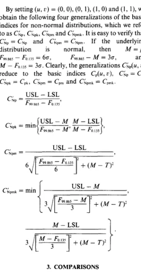
(0, 1), (1, 0) and (1, 1), we obtain the four generalizations of the basic indices for non-normal distributions, which can be expressed explicitly as the following. We refer to these four generalizations as Chp, Chpk,

CNp,,

and CNpmk- USL - LSL CNp - - F99 865 - - F0.135' C , ~ p k = m i n { USL__-_M . M - L S L

If99.8652Fo.1351'I.F~9.8652-Z3~]~

USL - LSL CNp m ~ CNp.,k = min I U S L - - _ M ,

'h 3~[F9~I~6'

~ F°"']: + (M-Ty

2. CAPABILITY INDICES FOR NON-NORMAL DISTRIBUTIONS

To accommodate cases where the underlying distributions may not be normal, we consider the following generalizations of

Co(u, v),

which we refer to as

Cup(U, v).

The generalizations

Cup(u, v)

can be defined as the following (in superstructure form), where F, is the ~th percentile, M is the median of the distribution, m = ( U S L - L S L ) / 2 , /l and a are process mean and process standard deviation, and b/, b' ~ 0.

d - u l M - m [

C.p(u,

v) = (2)

+ v ( m - T)-'

Thus, in developing the generalizations

Csp(u, v)

we have replaced the process standard deviation, a, by (F99.865 - F0t35)/6 in the definition of

Co(u, v).

The idea behind such replacements is to mimic the property of the normal distribution for which the tail probability outside the _+ 3a limits from/~ is 0.27%, thus assuring that if the calculated value of

CNp(u,

v) = i (assuming the process is well-centered) the probability that process is outside the specification interval (LSL, USL) will be negligibly small. We also have replaced the process mean, /~, by the process median M since the process median is a more robust measure of central tendency than the process mean, particularly for skew distributions with long tails. By setting the parameter values (u, v) = (0, 0),

M - LSL 1 .

JI

T

3 F.9 65 F0,35 + ( g - T):

In general, the relationships among the four generalizations can be established as the following: CNp,, = CNp{1 + [ ( M -

T)/a"]2} -'2,

and CNpmk{1 + [ ( M -

T)/a"] 2}

':, where

a"

= (F99865 -- F0,35)/6 The ranking of the four generalizations in terms of sensitivity to departure of the process median from the target value, from the most sensitive to the least sensitive are: (1) CNpmk, (2) CNp~,, (3) CNpk and (4) CNp. For symmetric tolerances, we can show that Cup~ = (1 - k) CNp and Cup,,k = (1 -- k) Chpm, where

k = [M - Tl/d

is the departure ratio. If the process is

on-target, then clearly k = 0 ( M = T) and

CNp = CNpk = Cup,,, = CNp,,k =

d/3a".

On the other hand, if the underlying distribution is normal, then M = p, and a " = a. Clearly, the generalizations

Cup(u,v)

reduce to the basic indices

Cp(u,v)

and Cup = Cp, CNpk : Cpk, CNpm : Cpm and

Cupmk = Cpmk.

Pearn and Kotz [5], and Pearn and Chen [13] applied Clements' method [14], and proposed esti-

mators for calculating

Cp(u,v)

for non-normal

Pearsonian distributions. The proposed estimators are essentially based on the estimates Up and

Lp

for the two percentiles F99865 and F0t,, utilizing estimates of the mean, standard deviation, skewness and kurtosis. The indices in which those estimators correspond to can be expressed as:

(3)

C~p(u,

v) = (l -- u) USL - LSL X 6 /[Fo9's6' 6 F°"35-12

+ v ( M - - T )

2 + u × m i n ~ U S L T _ M ,

13/[u'°"6' - MT

L VL

-3- j

M-_LSL_

} .

(3)

By setting (u, v) = (0, 0), (0, 1), (1, 0) and (1, 1), we obtain the following four generalizations of the basic indices for non-normal distributions, which we refer to as C;~p, C;~pk, C(qpm and C(~pmk. It is easy to verify that C(~p = Csp and C{~pm = CNpm. If the underlying

distribution is normal, then M = #,

F99.865 - - F0135 = 6a, F99.865 - - M = 3a, and

M - F0u5 = 3a. Clearly, the generalizations

C~p(u, v)

reduce to the basic indices

Cp(u,v), C~o = Co,

CNpk : Cpk, C{~pm : Cpm and CIqpmk = Cpmk, USL - LSL CNp -- F99865 -- F0.,5' . ( U S L - M M - LSL~ C~pk = m l n ~ . ~

M ' M -

Fo.l,,J' USL - LSL Fi 2

6&6 o,,35]

C~pmk = min ~ U.__SL__.Z M

l

3 / F F 9 9 8 6 5 - M12

4L x -A+(M-

M - LSL 1 . . . . I " 0.,35] + ( M - - T ) 2

ry

3. COMPARISONS

To compare the two generalizations

CNp(u, v)

and

C~p(u,

v) with the basic indices

Cp(u, v),

we consider the following example consisting of three processes A, B and C (heavily skewed with long tails) (Fig. 1). The distributions of processes A, B and C are Z~ (chi-square distribution with degrees of freedom 2). The process characteristics are summarized in Table 1 (aA = aB = ac = 2.00). We note that process B is on-target, whereas processes A and C are severely off-target. In fact, for process A the process mean

3 0 37 44

Fig. 1. Distributions of processes A, B and C.

#A = LSL = 30 and for process C the process mean #c = USL = 44. Process capabilities for A and C are far below the minimum requirements (capable) set in the electronic industries.

Table 2 is a comparison between Cp(u, v) and

CNp(u, v)

on the three processes A, B and C depicted in Fig. 1. The index values of Cp, Cpk, Cpm and Cpmk given to processes A and C are the same [(1.17, 0.00, 0.32, 0.00) for A and C]. Both processes A and C are severely off-target. However, the proportion of non-conforming for process A is 63%, which is significantly greater than that for process C (37%). Obviously, the basic indices Cp(u, v) inconsistently measure process capabilities of processes A and C in this case. On the other hand, the proposed generalizations

CNp(u, v)

clearly differentiate processes A and C by giving smaller values to A and larger values to C (excluding CNp which never considers process median and, hence, provides no sensitivity to process departure at all).

In the following, we compare the two generalizations

CNp(u,

v), and

C~r(u, v)

based on a process characteristic discussed in Choi and Owen [15], which is related to loss functions. As we pointed out earlier, the generalizations

Cup(u, v)

obtain the maximal values when the process is on-target (M = T). On the other hand, the generalizations

C~p(u, v)

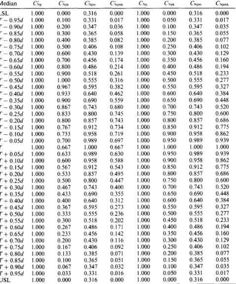
obtain the maximal values when the process is off-target (M < T). To illustrate this point, we consider the following example with manufacturing specifications L S L = T - d , U S L = T + d .

Table 3 displays the values of

CNp(u,v)

and

C~p(U,V)

for various values of M, with fixed percentile deviation F99.865 - - F0)35 = 2d. We note that

in Table 3, the generalizations CNp(u,v) are

maximized by M = T (Cyp = CNpk = CNpm =

CNo,,k

= 1.00). On the other hand, the generalizations

C(~p(u, v)

are maximized by M = T - 0.5 d for C~rk and by M = T - 0 . 2 5 d for C'~pm~ (the process is off-target).

Table 1. Characteristics of processes A, B and C

Process p M a F0 135 F99 865

A 30.00 29.39 2.00 28.00 41.22

B 37.00 36.39 2.00 35.00 48.22

(4)

Table 2. A comparison between C.p (u, v) and Cp (u, v) Process Cr Cpk Cp,,~ Cp,,k CNp CNpk CN0,, CNpm~ A 1.17 0.00 0.32 0.00 1 . 0 6 - 0 . 0 9 0.29 -0.03 B 1.17 1.17 1.17 [.17 1.06 0 . 9 7 1.02 0.93 C 1.17 0.00 0.32 0.00 1.06 0 . 0 9 0.35 0.03

4. ELECTROLYTIC CAPACITOR MANUFACTURING

T o illustrate h o w the generalizations CNp(U, v) may be applied to actual data collected from the factories, we present a case study on an a l u m i n u m electrolytic capacitor m a n u f a c t u r i n g process. The case which we studied was taken from an electronics c o m p a n y (located in Taiwan) w h o is a m a n u f a c t u r e r a n d supplier o f a l u m i n u m electrolytic capacitors supplying various kinds o f capacitors including n o n - p o l a r i z e d capacitors (with radial or axial leads), a n d bi-polarized capacitors (with radial or axial leads).

N o n - p o l a r i z e d capacitors are designed to be used in crossover n e t w o r k s with high-pitch, median-pitch a n d low-pitch s o u n d s in high-fidelity audio speaker systems. The m a n u f a c t u r i n g specifications set o n the p e r f o r m a n c e characteristics for non-polarized capacitors are described in the following: the operating t e m p e r a t u r e range is between - 4 0 a n d + 8 5 ° C ; the voltage range is between 50 a n d 100V; the capacitance specified by the customers can be any value between 1 and 1000 p F ; the leakage current is no greater t h a n max {0.03

CV,

3/zA} after 5 min application o f the rated voltage, where C = the rated capacitance (in/~F); a n d V = D C working voltage at 20"C.

Bi-polarized capacitors are designed for horizontal defection c u r r e n t in TV sets with high frequency a n d high ripple current flows, which have the a d v a n t a g e o f small dissipation factors at high frequency. The m a n u f a c t u r i n g specifications set on the p e r f o r m a n c e characteristics for bi-polarized capacitors are described in the following: the

Table 3. A comparison between CNo (u, v) and CG (u, c) (with production specifications U S L = T + d , L S L = T - d ) Median CG CG~ CNpm C~qpmk CN D CNpk CNpm CNpmk LSL 1.000 0.000 0.316 0.000 1.000 0.000 0.316 0.000 T - 0.95d 1.000 0.I00 0.331 0.017 1.000 0.050 0.331 0.017 T - 0.90d 1.000 0.200 0.347 0.036 1.000 0.100 0.347 0.035 T - 0.85d 1.000 0.300 0.365 0.058 1.000 0.150 0.365 0.055 T - 0.80d 1.000 0.400 0.385 0.082 1.000 0.200 0.385 0.077 T - 0.75d 1.000 0.500 0.406 0.108 1.000 0.250 0.406 0.102 T - 0.70d 1.000 0.600 0.430 0.139 1.000 0.300 0.430 0.129 T - 0.65d 1.000 0.700 0.456 0.174 1.000 0.350 0.456 0.160 T - 0.60d 1.000 0.800 0.486 0.214 1.000 0.400 0.486 0.194 T - 0.55d 1.000 0.900 0.518 0.261 1.000 0.450 0.518 0.233 T - 0.50d 1.000 1.000 0.555 0.316 1.000 0.500 0.555 0.277 T - 0.45d 1.000 0.967 0.595 0.382 1.000 0.550 0.595 0.327 T - 0.40d 1.000 0.933 0.640 0.462 1.000 0.600 0.640 0.384 T - 0.35d 1.000 0.900 0.690 0.559 1.000 0.650 0.690 0.448 T - 0.30d 1.000 0.867 0.743 0.680 1.000 0.700 0.743 0.520 T - 0.25d 1.000 0.833 0.800 0.745 1.000 0.750 0.800 0.600 T - 0.20d 1.000 0.800 0.857 0.743 1.000 0.800 0.857 0.686 T - 0.15d 1.000 0.767 0.912 0.734 1.000 0.850 0.912 0.775 T - 0.10d 1.000 0.733 0.958 0.719 1.000 0.900 0.958 0.862 T - 0.05d 1.000 0.700 0.989 0.697 1.000 0.950 0.989 0.939 T 1.000 0.667 1.000 0.667 1.000 1.000 1.000 1.000 T + 0.05d 1.000 0.633 0.989 0.630 1.000 0.950 0.989 0.939 T + 0.10d 1.000 0.600 0.958 0.588 1.000 0.900 0.958 0.862 T + 0.15d 1.000 0.567 0.912 0.543 1.000 0.850 0.912 0.775 T + 0.20d 1.000 0.533 0.857 0.495 1.000 0.800 0.857 0.686 T + 0.25d 1.000 0.500 0.800 0.447 1.000 0.750 0.800 0.600 T + 0.30d 1.000 0.467 0.743 0.400 1.000 0.700 0.743 0.520 T + 0.35d 1.000 0.433 0.690 0.355 1.000 0.650 0.690 0.448 T + 0.40d 1.000 0.400 0.640 0.312 1.000 0.600 0.640 0.384 T + 0.45d 1.000 0.367 0.595 0.273 1.000 0.550 0.595 0.327 T + 0.50d 1.000 0.333 0.555 0.236 1.000 0.500 0.555 0.277 T + 0.55d 1.000 0.300 0.518 0.202 1.000 0.450 0.518 0.233 T + 0.60d 1.000 0.267 0.486 0. l 71 1.000 0.400 0.486 0.194 T + 0.65d 1.000 0.233 0.456 0.142 1.000 0.350 0.456 0.160 T + 0.70d 1.000 0.200 0.430 0.116 1.000 0.300 0.430 0.129 T + 0.75d 1.000 0.167 0.406 0.092 [ .000 0.250 0.406 0.102 T + 0.80d 1.000 0.133 0.385 0.071 1.000 0.200 0.385 0.077 T + 0.85d 1.000 0.100 0.365 0.051 1.000 0.150 0.365 0.055 T + 0.90d 1.000 0.067 0.347 0.032 1.000 0.100 0.347 0.035 T + 0.95d 1.000 0.033 0.331 0.016 1.000 0.050 0.331 0.017 USL 1.000 0.000 0.316 0.000 1.000 0.000 0.316 0.000

(5)

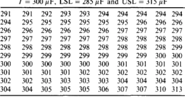
Table 4. Non-polarized (NP) with radial leads; capacitance T = 300/~F, LSL = 285/~F and USL = 315/tF 292 293 294 294 294 294 294 294 295 295 295 295 295 295 295 296 296 296 297 297 297 297 297 298 298 298 298 298 298 298 299 299 299 300 300 300 300 300 301 301 301 301 302 302 302 302 302 302 302 303 303 303 303 303 303 304 304 304 304 304 305 305 305 305 305 305 306 306 306 306 306 306 307 307 307 308 308 308 308 309 309 309 309 309 309 310 310 310 311 312 312 313 313 313 313 315 316 319 320 324

operating temperature range is between - 4 0 and + 85°C; the voltage range (specified by the customers) should not be greater than 50 V; the capacitance specified by the customers can be any value between 1 and 1000/~F, leakage current is no greater than max {0.03

CV,

3/~A} after 5 min application of the rated voltage, where C = the rated capacitance (in ~F) and V = DC working voltage at 20°C; and the capacitance at - 4 0 ° C should not be less than 80% of the capacitance at 20°C.

In the manufacturing factory, the raw material aluminum-foil rolls shipped directly from the supplier are first cut into narrow aluminum-foil rolls with appropriate width (depending on the sizes of the capacitors to be made). The lead wire (aluminum for the head and copper for the legs) is then cleaned and stitched on to the aluminum foil sheet. Two piles of aluminum-foil sheet (with the lead wire stitched on) are rolled with two piles of paper to form the capacitor interior. The capacitor interior is then soaked into the electrolytic solution, loaded on to the automatic assembly machine, and assembled with the aluminum case, rubber end seal and PVC sleeve. The drying and cleaning work for the rubber end seal and copper-lead are processed by automatic machines before the assemblies. Finally, the assembled capacitor is loaded on to the shelf, and completed by the aging process to produce the capacitors.

The upper and lower specification limits, USL and LSL, for a particular model of aluminum non-polarized capacitor (with radial leads) were set to 285 and 315 (in # F). The target value is the mid-point between the two specification limits, which is 300. The collected sample data (a total of 100 observations) are displayed in Table 4. This is a non-normal distribution (based on the 100 observations).

5. CAPABILITY CALCULATIONS

Chang and Lu [16] considered a percentile method to calculate F99~65 and F0.,5, and the median M, and applied Clements' method to obtain the percentile estimators for the three indices C~p, C~pk and C~pm. Extending their method to the generalizations

CNp(u, v),

we can construct a superstructure for the estimators of

CNp(u, v),

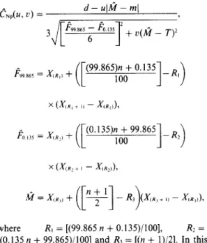
which may be expressed as the following: ~ . . ( u . v) =

jp

d - ul~t - m[

]2

3 9865 - Fo.135 _g- _{+ v ( ~ - T ) 2}

{F(99.865)n + O'135]_R, )

/1~99 865 =

X(RI) "]-

r66

X (/~/'[RI + i t - X{/~])), (0.135)n + 99.865 x (X~,,:+, - X . , . ) , where R, = [(99.865 n + 0.135)/100], R: = [(0.135 n + 99.865)/100] and R3 = [(n + 1)/2]. In this setting, the notation [R] is defined as the greatest integer less than or equal to the number R, and x~j~ is defined as the ith order statistic.

For the 100 observations, X~ = 292, X~991 = 320 and X,0~= 324. To obtain the values of the estimators (~sp(u, v) for the proposed generalizations

C,~(u,v),

we first calculate the three sample percentiles obtaining F0.,5 = 292.1, F99.865 = 323.5 and

!Q = 303. Then, we substitute these values into the definition of CNp(u, v) obtaining CNp = 0.96, CNpk = 0.76, (~Npm = 0.83 and ~'Npmk = 0.66.

We note that the C'Np value is less than 1.00 and the process is "inadequate"; it indicates that the process is not adequate with respect to the given manufacturing specifications, either the process variation needs to be reduced or the process median needs to be shifted closer to the target value. In fact, there are four observations (316, 319, 320 and 324) falling outside the specification interval (LSL, USE) and the proportion of non-conforming is 4%.

The quality condition of such a process was considered to be unsatisfactory in the company. Some quality improvement activities, involving Taguchi's parameter designs, were initiated to identify the significant factors causing the process failing to meet the company's requirement. Conse- quently, machine settings for the aging process, as well as other process parameters were adjusted. To check whether the adjusted process was satisfactory, a new sample of 100 from the adjusted process was collected yielding the following measurements (Table 5). Specifications, process capability requirements remained the same. We performed the same calculations over the new sample of 100 observations. We obtained CNp = 1.39, t~Np~ = 1.30, (~Npnl = 1.34, and CNp,,k = 1.25. We note that the new (adjusted) process has zero defectives. As a result, problems were successfully resolved and the quality of this manufacturing process improved significantly.

(6)

Table 5. Non-polarized (NP) with radial leads; capacitance T = 300pF, LSL = 2 8 5 p F and USL = 315 #F 291 291 292 293 293 294 294 294 294 294 294 295 295 295 295 295 295 296 296 296 296 296 296 296 296 296 297 297 297 297 297 297 297 297 297 297 298 298 298 298 298 298 298 298 298 298 298 298 298 299 299 299 299 299 299 299 299 299 300 300 300 300 300 300 300 300 301 301 301 301 301 301 301 301 302 302 302 302 302 302 302 302 303 303 303 303 304 304 304 304 304 304 305 305 305 306 307 307 310 313 6. CONCLUSIONS

In this paper, we c o n s i d e r e d two generalizations o f the basic indices Cp(u, v), which we referred to as CNp(u, v) a n d C~p(U, v), to cover n o n - n o r m a l distributions. If the u n d e r l y i n g d i s t r i b u t i o n is n o r m a l , t h e n b o t h generalizations CNp(u, v) a n d C~r,(u, v) reduce to the basic indices Cp(u,v). T h e generalizations CNo(u, v) are c o m p a r e d with the basic indices Cp(u, v) a n d C~p(u, v). The results indicated t h a t the p r o p o s e d generalizations CNp(u, v) are m o r e c o n s i s t e n t a n d accurate t h a n Cp(u,v) a n d C~,p(uo v) indices in m e a s u r i n g process capability. In a d d i t i o n , we considered a n e s t i m a t i o n m e t h o d based on sample percentiles to calculate the p r o p o s e d generalizations CNp(U, v). C o m p u t a t i o n s for o b t a i n i n g the e s t i m a t o r s do n o t require a n y a s s u m p t i o n s o n the u n d e r l y i n g d i s t r i b u t i o n s or statistical tables.

W e also presented a case study on a n a l u m i n u m n o n - p o l a r i z e d c a p a c i t o r m a n u f a c t u r i n g process to illustrate h o w the generalizations CNp(u, v) m a y be applied to actual d a t a collected f r o m the factories. The calculations are easy to u n d e r s t a n d , straightfor- w a r d to apply a n d s h o u l d be e n c o u r a g e d for i n - p l a n t applications.

REFERENCES

1. Hoskins, J., Stuart, B. and Taylor, J., A Motorola commitment: a six sigma mandate. The Motorola Guide

to Statistical Process Control./or Continuous Improve- ment Towards Six Sigma Quality, 1988.

2. Rado, L. G., Enhance product development by using capability indexes. Quality Progress, 1989, 22(4), 38-41. 3. Hubele, N. F., Montgomery, D. C. and Chih, W. H., An application of statistical process control in jet-turbine component manufacturing. Quali O, Engng,

1991, 4(2), 197-210.

4. Noguera, J. and Nielsen, T., Implementing six sigma for interconnect technology. ASQC Quali O, Congress Trans., Nashville, 1992, pp. 538 544.

5. Pearn, W. i . and Kotz, S., Application of Clements' method for calculating second and third generation process capability indices for non-normal Pearsonian populations. Quality Engng, 1994, 7(1), 139-145. 6. Lyth, D. M. and Rabiej, R. J., Critical variables in

wood manufacturing's process capability: species, structure, and moisture content. Quality Engng, 1995, 8(2), 275 281.

7. V/innman, K., A unified approach to capability indices. Statistica Sinica, 1995, 5, 805-820.

8. Kane, V. E., Process capability indices. J. Quail O, Tech., 1986, 18(1), 41-52.

9. Chan, L. K., Cheng, S. W. and Spiring, F. A., A new measure of process capability: Cpm. J. Qualio' Tech.,

1988, 20(3), 162 175.

10. Pearn, W. L., Kotz, S. and Johnson, N. L., Distributional and inferential properties of process capability indices. J. Quality Tech., 1992, 24(4), 216-233.

11. Chan, L. K., Cheng, S. W. and Spiring, F. A., The robustness of the process capability index, Cv, to departures from normality. Statistical Theory and Data Analysis H, ed. K. Matusita. North Holland, 1988, pp. 223 239.

12. Gunter, B. H., The use and abuse of Cp~. Part 3. Quality Progress, May, 1989, 79 80.

13. Pearn, W. L. and Chen, K. S., Estimating process capability indices for non-normal Pearsonian populations. Quality & Reliability Engng Int., 1995, 11(5), 386-388.

14. Clements, J. A., Process capability calculations for non-normal distributions. Quality Progress, September 1989, 95 100.

15. Choi, B. C. and Owen, D. E., A study of a new capability index. Communications in Statistics--Theory and Methods, 1990, 19(4), 1231-1245.

16. Chang, P. L. and Lu, K. H., PCI calculations for any shape of distribution with percentile. Quality WorM, technical section, September 1994, 110-114.