MASS TRANSIT ROUTE NETWORK DESIGN USING GENETIC ALGORITHM

Publisher: Taylor & Francis

Informa Ltd Registered in England and Wales Registered Number: 1072954 Registered office: Mortimer House, 37-41 Mortimer Street, London W1T 3JH, UK

Journal of the Chinese Institute of Engineers

Publication details, including instructions for authors and subscription information: http://www.tandfonline.com/loi/tcie20

Mass transit route network design using genetic

algorithm

Jin‐Yuan Wang a _{& Chih‐Ming Lin} b a

Department of Transportation Technology and Management , National Chiao Tung University , Hsinchu, 300, Taiwan, R.O.C. Phone: 886–3–5725804 Fax: 886–3–5725804 E-mail:

b

Department of Transportation Technology and Management , National Chiao Tung University , Hsinchu, 300, Taiwan, R.O.C.

Published online: 04 Mar 2011.

To cite this article: Jin‐Yuan Wang & Chih‐Ming Lin (2010) Mass transit route network design using genetic algorithm,

Journal of the Chinese Institute of Engineers, 33:2, 301-315

To link to this article: http://dx.doi.org/10.1080/02533839.2010.9671619

PLEASE SCROLL DOWN FOR ARTICLE

Taylor & Francis makes every effort to ensure the accuracy of all the information (the “Content”) contained in the publications on our platform. However, Taylor & Francis, our agents, and our licensors make no

representations or warranties whatsoever as to the accuracy, completeness, or suitability for any purpose of the Content. Any opinions and views expressed in this publication are the opinions and views of the authors, and are not the views of or endorsed by Taylor & Francis. The accuracy of the Content should not be relied upon and should be independently verified with primary sources of information. Taylor and Francis shall not be liable for any losses, actions, claims, proceedings, demands, costs, expenses, damages, and other liabilities whatsoever or howsoever caused arising directly or indirectly in connection with, in relation to or arising out of the use of the Content.

This article may be used for research, teaching, and private study purposes. Any substantial or systematic reproduction, redistribution, reselling, loan, sub-licensing, systematic supply, or distribution in any

form to anyone is expressly forbidden. Terms & Conditions of access and use can be found at http:// www.tandfonline.com/page/terms-and-conditions

MASS TRANSIT ROUTE NETWORK DESIGN USING GENETIC

ALGORITHM

Jin-Yuan Wang* and Chih-Ming Lin

ABSTRACT

The mass transit route network design (MTRND) problem is a bi-level NP-hard problem and difficult to solve for a global optimum solution. This paper proposes a genetic algorithm for solving the MTRND problem. In the proposed algorithm, two smart generating methodologies are formulated to achieve a better searching space for the initial feasible solution. An efficient network model, a gene repairing strategy and a redundancy checking mechanism were applied to minimize the computation time. Improved fitness function was embedded with the passenger assignment model and utilized to improve the quality of the solution. The proper combination of cross-over operators and mutation operators was found for the MTRND. The proposed algorithm was tested with the current MRT network in Taipei as a specimen. Results indicate that the proposed algorithm is effective in solving real-world problems. Key Words: mass transit systems, passenger assignment, network design, genetic

algorithm.

*Corresponding author. (Tel: 5725804; Fax: 886-3-5725804; Email: [email protected])

The authors are with the Department of Transportation Technology and Management, National Chiao Tung University, Hsinchu 300, Taiwan, R.O.C.

I. INTRODUCTION

The route network design problem for mass rapid transit (MTRND) involves determining a set of ser-vice routes and the associated headway, minimizing system operating costs and passenger travel costs subject to relevant operational constraints. Conventionally, this task is done manually in two stages. The de-signer in the first stage transfers the given demand matrix into network link flows based on rules of thumb. Then an initial solution is obtained by accommodat-ing certain system requirements (such as policy ser-vice level). Actual link flows are estimated in the second stage by simulating passengers’ route choice behavior. If the flow exceeds the capacity on some links, the designer must make some modifications, affecting each link cost. After adjusting the solution, passengers may have different route choices and link flows may change again. The process repeats until all constraints are satisfied.

The abovementioned process relies heavily on intuitive principles based on the designer’s own experiences. The process is designer-dependent and lacks consistency and reliability. Therefore, more efficient MTRND methods are desired.

MTRND is a special type of transit network de-sign and frequencies setting problem (TNDFSP). There are various modeling and solution techniques for TNDFSP. Readers may refer to recent works by W i r a s i n g h e ( 2 0 0 3 ) , C e d e r ( 2 0 0 3 ) , F a n a n d Machemehl (2004) and Guihaire and Hao (2008) for comprehensive reviews. However, most of these past works focus on urban bus systems (Guan et al., 2006) with little emphasis on MTRND. Zhao and Zeng (2006) treated MRT as a express bus system, and solved for it together with other transit systems. Guan

et al. (2006) developed an integrated model for

si-multaneous optimization of transit line configuration and passenger line assignment in a general network to balance transit line operating cost, passenger trans-fer times, and total travel distance. The model is for-mulated as a binary integer programming problem, illustrated with a couple of minimum spanning tree networks and solved by the standard branch and bound method. The model was tested with a simplified ver-sion of the general Hong Kong mass transit railway

network with only 9 nodes and 10 links.

In addition to most of the TNDFSP models, the MTRND needs more MRT-specialized characteristics such as platform capacity, congestion penalties for overloaded trains, no missed trips, all stations and segments must be served, and an exact fleet size. Thus an MTRND model which can reflect real world con-siderations and an efficient and robust solution algo-rithm is needed.

Because the genetic algorithm has the ability to do global searching, construct objective functions easily, add many constraints, and access variable net-work problems, this paper applies a genetic algorithm to resolve our proposed MTRND model.

We discuss the applications of GA on TNDFSP here since few studies before now have been directly related to MRTND. Guihaire and Hao (2008) pre-sented a comprehensive review of the crucial strate-gic and tactical steps of transit planning, including GA-based models for TNDFSP. Tom and Mohan (2003) proposed an SRFC model which incorporates line frequency as a variable, and simultaneously de-termines transit line routes and frequencies, with the objective of minimizing both operating costs and pas-sengers’ total travel time. A sample network defined by 75 nodes and 125 links (Chennai, India) has been established to demonstrate the performance of the model. Agrawal and Tom (2004) proposed two SRFC-based parallel GA models. The models were tested by a large urban (New Delhi, India) route net-work with 1,332 nodes and 4,076 links for computa-tion time, speed, and efficiency. Fan and Machemehl (2004, 2006a) proposed a genetic algorithm tested by a 160 node, 418 link example network to systemati-cally examine the underlying characteristics of the optimal bus TNDFSP with variable transit demand. Finally, the application of Genetic algorithms to the TNDFSP was studied by Zhao and Zeng (2006a). A stochastic search scheme based on a simulated an-nealing and GA search method has been developed to obtain results for large-scale practical problems.

This paper is organized as follows. First, a bi-level programming model of MTRND is presented together with a network representation. Then the pro-posed genetic algorithm is described, followed by a case study based on the current TRTC mass transit network to illustrate real-world application of the pro-posed model and algorithm. Conclusions are given in the last section.

II. PROBLEM STATEMENT OF MTRND The MTRND can be represented as the follow-ing bi-level mathematical model:

Minu F(u, v(u)) (1)

s.t.

G(u, v(u)) ≤ 0, (2) where v(u) is implicitly defined by

Minv f (u, v) (3)

s.t.

g(u, v) ≤ 0. (4)

F is the objective function of the upper-level

problem, which minimizes operating costs and pas-senger traveling costs. u represents a decision vec-tor of the upper-level problem (targeting designer), which is a set of routes and the associated headway;

G is the constraint set of the upper-level problem, such

as level of service, link capacity, network connectivity, fleet size, and limits of headway. f is the objective function of the lower level problem (targeting passenger), which minimizes travel costs. v is a de-cision vector of the lower-level problem, represent-ing a set of link flows. g is the flow conservation constraint for the lower-level problem.

This work assumes that for any given u, there is a unique equilibrium solution v(u) obtained from the lower-level problem. The v(u) is called the reaction function. It is in effect a nonlinear equity constraint of the upper-level problem and a congestion penalty of the objective function F; thus MTRND is intrinsi-cally non-convex, which is an NP-hard problem and difficult to solve optimally (Ben-Ayed et al., 1988; Yang et al., 1994; Constantin and Florian, 1995; Yin, 2000; Gao et al., 2005; Chiou, 2005).

The lower-level problem represents the passenge’s route choice behavior in response to costs decided by the upper-level decision maker. The current work assumes that passengers make their route choices in a user-optimal manner; hence the lower-level prob-lem can be formulated as a standard user equilibrium passenger assignment problem, or a stochastic user equilibrium problem (Sheffi, 1985).

III. NETWORK REPRESENTATION Figure 1(a) represents a nine-station, eight-seg-ment mass transit network. Fig. 1(b) shows five avail-able routes in the candidate set. For example, route 1 represents the 1-4-7-8-7-4-1 travel path. Trains stop at each station and reverse at terminal stations (1 and 8). Round trip time and round trip distance of route 1 is RT1 and RL1. If route 1 is chosen and its associ-ated frequency is F1, then s1 is set to 1 and the num-ber of trains required by route 1 TS1 is calculated by Eq. (5).

TS1 = |s1 × RTi× Fi| (5)

Traditionally, a mathematical programming model must consider all possible routes and use bi-nary variable si to decide whether to choose the ith

route or not. Then constraint (6) ensures that the to-tal number of trains used does not exceed the fleet size TRC.

Σ

Figure 1(c) represents the network model for this example, with five link types based on various pas-senger activities described in Table 1. Nodes corre-spond to exits, entrances, boarding, alighting, and platform. No costs are associated with nodes. Also,

the exit/entrance node (i.e. stations 1~9) will be the sink/source of trips in the passenger assignment problem.

For example, the bold solid line of Fig. 1(c) de-picts passenger movements from station 1 to station 6. A passenger enters station 1, walks to the platform, waits, boards the train of route 1, and alights at the platform of interchange station 4. If route 4 and 5 are chosen simultaneously, he may take route 4 to reach station 6 directly, or alternatively, he may take route 5 to station 5, alight at the platform, and then transfer to route 4 to station 6. Making transfers takes time and is inconvenient. Passenger assignment prob-lems should therefore take into account in-vehicle travel time as well as transfer time. Transfer time from one route to another in the example mentioned

d-type link 2 ₄ 7 8 ₉ (b) 1 2 3 4 5 6 7 8 9 (4) (1) (3) (2) (5) (a) 1 2 3 4 5 6 7 8 9 (c) 3 5 ₆ e-type link a-type link c-type link b-type link Exit/Entrance Board/Alighting Platform 1 : Exit/Entrance : Platform : Boarding/Alighting : Link

Fig. 1 A 9-station mass transit network example

above can be estimated exactly by additional links of alighting, waiting, and boarding. Therefore, these five link types can represent passenger movements adequately and reasonably, thus simplifying the math-ematical programming problem.

The free travel cost of a-type and e-type links in Table 1 represents the time walking on the un-con-gested walk lane. The free travel cost of the b-type link is the waiting time at the platform. Suppose the arrival rate of passengers is a normal distribution. Then the free travel cost of a b-type link is half the headway of the associated route (Turmquist, 1978). The free travel cost of the c-type link is in-vehicle time between two adjacent stations. Depending on the associated route timetable, free travel cost is usu-ally constant. Capacities of the a-type and e-type link are the design capacities of walk lanes. The capaci-ties are calculated adequately in the construction phase of mass transit system stations and can be col-lected easily from the associated design documents. Capacities of the b-type and d-type link are design capacity parts of the associated platform. The ca-pacity of the c-type link is the caca-pacity sum of trains of the associated route passing through the origin node, which is decided by the associated route headway.

Some links may be overloaded and become crowded after the passenger assignment phase. Such a condition causes passenger inconvenience on the links. Passenger total cost should therefore take into account free travel cost as well as congestion penalty. The link travel time function suggested by the U.S. Bureau of Public Roads is used (Lee and Hsieh, 2002).

TC(x) = t0× 1 + 0.15 × xv

c

4

, (7)

where TC = passenger travel cost with congestion pen-alty on the link; t0 = free travel cost when the link is not congested; x = passenger volume on the link; vc =

link capacity described in Table 1.

The following notable assumptions are made in the formulation:

1. The MTRND is a long-term plan. The O-D matrix of the mass transit system is not affected by the plan result.

2. The fare depends on the shortest distances from origin stations to destination stations. Passenger cost affected by routes and associated headway is travel time and congestion penalty.

3. The MTRND focuses on a peak hour plan. Route headway of non-peak hours is set to policy headways to perform at a required level of services.

4. Trains stop at every associated route station, and dwelling time and turnover time are constant. Thus the round distance and time of routes RLi and RTi

are constant.

5. Train capacities are the same and constant. 6. Peak hour passengers are commuters with the same

time values. They act rationally and know all rel-evant travel cost information, and travel the short-est paths from original stations to dshort-estination stations.

IV. FORMULATION OF MTRND

The MTRND problem stated in the previous sec-tion can be formulated as a nonlinear mixed-integer bi-leveling programming model shown below:

Min α×

Σ

Σ

Σ

Σ

Σ

Σ

Σ

Table 1 Five link types of passengers’ movement

Link type Movement of passengers Free travel cost Capacity

a Enter the origin station and Walking time when the Design capacity of walk lane walk to the platform walk lane is not congested

b Wait on the platform and Waiting time Design capacity of platform board the train

c In the train In-vehicle time Crresponding route capacity d Alighting Alighting time when the Design capacity of platform

platform is not congested

e Walk out on the platform and Walking time when the walk Design capacity of walk lane exit the destination station lane is not congested

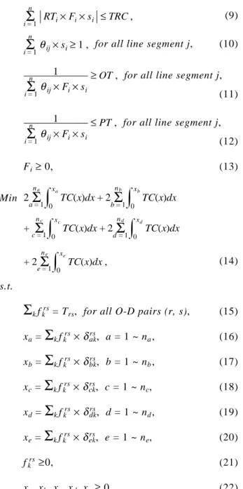
RTi× Fi× si

Σ

Σ

≥ 1 , for all line segment j, (10)

1 θij

Σ

≥ OT , for all line segment j,

(11) 1 θij

Σ

≤ PT , for all line segment j,

(12) Fi≥ 0, (13) Min 2

Σ

Σ

Σ

Σ

Σ

Σ

xa =

Σ

Σ

Σ

Σ

Σ

where α = unit operating cost per train-km; β = de-preciation per train-hour; γ = passenger’s in-vehicle time cost per hour; λ = weight which is decided by designer; the other symbols are described in the no-tation section.

The objective function (8) is the generalized cost of the mass transit system and passengers, measured in monetary cost. It contains three items. The first item reflects the energy cost, which is the product of total trip distance of all routes and the conversion parameter α. The second item reflects the deprecia-tion cost, which is the product of total trip time of all routes and the conversion parameter β. The third item reflects the travel cost, which is the product of total time value of all passengers and the conversion pa-rameter λ.

Constraint (9) limits the sum of trains used by routes within the fleet size. Constraint (10) is used to ensure that all stations and line segments are served. Constrains (11)-(12) are used to ensure that all line segment frequencies between every two adjacent sta-tions are in the minimum to maximum headway range. Constraints (14)-(22) denote the lower-level MTRND problem, a passenger assignment problem. Both the objective function (14) and the third item of Eq. (8) sum up travel cost of all link types. Based on the study of Chang and Guo (2007), the value of out-of-vehicle time (i.e. a, b, d and e-type links) is as-sumed as two times that of in-vehicle time (i.e. c-type links). Constraints (15)-(22) are traditional flow con-servation constraints.

The aforementioned problem is NP-hard because its upper-level problem is an NP-hard set-covering problem and the reaction function TC(x) is a non-lin-ear function.

V. PROPOSED SOLUTION ALGORITHM Genetic algorithms prove to be very effective for solving bi-level problems (Yin, 2000). The com-plicated network structure and large number of con-straints and variables make it very difficult to obtain optimal MTRND solutions. Thus, heuristics, such as genetic methods (Guan et al., 2006), are often adopted to solve the problem approximately and efficiently. This work develops a genetic algorithm based on MTRND characteristics, and applies several improve-ment strategies to enhance solution quality and save computational time.

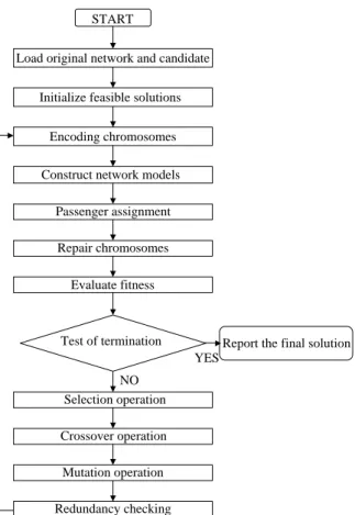
Figure 2 depicts the flowchart of the proposed MTRND genetic algorithm. Descriptions of impor-tant steps of the proposed algorithm follow.

1. Genetic Encoding

This coding scheme represents a chromosome (i.e., a solution) by a positive integer vector. Each individual chromosome gene represents the number of trains used by the corresponding route in the or-dered candidate route set. Hence, chromosome length is equal to the number of candidate routes. Although the proposed model requires pre-set candidate routes as input, these routes can be obtained easily from the operation manual. There is no need to determine these routes manually. A route is neglected if the associ-ated gene is assigned the value of 0. The ith route is chosen with the non-zero value fi of the associated

gene, and the associated frequency fi can be

calcu-lated easily by Eq. (23).

fi=

TSi

RTi

(23)

Figure 3 represents an n-gene chromosome. There are n routes in the chromosome. The number of trains used by the first route is 10, by the second route is 3, by the third route is 0 (hence the third route is not chosen), and so on. The sum of the gene val-ues is the number of trains used, which must not ex-ceed the pre-determined fleet size.

2. Initialize Feasible Solutions

The initial solutions are generated randomly based on the coding scheme described in section V.1 and should satisfy the hard constraints (9)-(12). A solu-tion violating any of them becomes an infeasible solusolu-tion. A number of infeasible solutions may appear before finding enough feasible solutions because of MTRND characteristics; and it takes some time to get enough feasible solutions. The current study develops two faster methods to generate enough feasible solutions according to operational experience: the 1-car method and the minimum-car method. The basic concept con-siders all candidate set routes and calculates their maxi-mum and minimaxi-mum trains. The 1-car method sets the minimum number of train routes to 1. The number of trains used by the chosen route is determined ran-domly between the maximum and the minimum. Af-ter all chromosome genes are generated this way,

constraints (9)-(12) are re-checked for feasibility. A feasible solution results if all constraints are satisfied. The steps of these two methods are described below:

(i) Set each route frequency in the candidate route set to 15. Compute the maximum number of trains used by each route TRimax using the

formu-lation given in Eq. (24).

TRimax = RTi× fi (24)

(ii) Compute the minimum number of trains used by each route TRimin as follows:

a. If the method is the 1-car method, let the mini-mum number of trains of each route be 1. b. If the method is the minimum-car method,

solve the passenger assignment problem by taking all candidate set routes into consider-ation and relax the constraints (9)-(12). After getting the maximum flow of each route Fimax,

compute each TRimin using Eq. (25).

TR_imin=Fi

max

TR_c , (25)

where TRc = capacity of each train.

(iii) Implement the following steps for each chromo-some, repeating these steps until there are enough feasible solutions.

a. For each gene in the chromosome, decide ran-domly whether each route is chosen or not. That is, decide whether each si is 1 or 0.

b. For each gene, if si is 1, decide TRi randomly

in the range between TRimin and TRimax.

Other-wise, let TRi = 0.

c. After all chromosome genes are generated, examine the chromosome by checking con-straints (9)-(12). The chromosome is a fea-sible solution if the constraints are satisfied. Otherwise abandon this chromosome and cre-ate another.

Based on operational experiences, because of the computation of TRimax by a frequency of 15/hr (i.e.

four minutes headway) and using TRimin as well, we

can decide the trains used by each route reasonably, thus getting a good initial solution search space. When each route is chosen and the number of needed trains is known, we can compute energy cost and de-preciation cost using the formulation given in Eq. (8).

Initialize feasible solutions

Evaluate fitness Encoding chromosomes Test of termination Selection operation Crossover operation Mutation operation Load original network and candidate

Passenger assignment START

Repair chromosomes Construct network models

Redundancy checking

Report the final solution YES

NO

Fig. 2 Flowchart of genetic algorithm

Chromosome Route 10 1 3 2 0 3 ... ... 4 n – 1 2 n

Fig. 3 An example of chromosome encoding

3. Construct Network Model

The algorithm takes the routes with non-zero number of trains into consideration and constructs a network model for each feasible solution, according to the previous section description. The passenger assignment model is utilized for the network model to get link flows. Then the travel cost using Eq. (8) formulation is computed. The constructed network model scale is not the same as the network model built by traditional mathematical programming methods. The latter considers all candidate set routes and takes more computation time. The former only considers part of the whole set, thus saving considerable com-putational time. This is one advantage of using a genetic algorithm to solve the MTRND problem. 4. Passenger Assignment

The passenger assignment model utilized by the algorithm is a standard deterministic Frank-Wolfe user equilibrium assignment model, based on Floyd’s shortest path method and all-or-nothing assignment method. The travel cost of each link is updated after each iteration assignment, using Eq. (7). Passenger travel cost is computed when the assignment is finished, using the Eq. (8) formulation to calculate solution fitness.

5. Repairing Strategy

A route in some feasible solutions may get very few trains, and hence have large headway and higher waiting cost. If alternative routes with higher capaci-ties can serve the same O-D pairs, the route with higher waiting cost may get zero flow after the pas-senger assignment step. The associated gene becomes useless. If a useless gene can be rejected and con-straints (9)-(12) satisfied simultaneously, we can im-prove fitness by reducing operation cost, and hence find a better solution. The method is a deep-search strategy.

This paper develops a repairing mechanism, to this end. All chosen route links are checked after the passenger assignment step. The associated gene value will be set to 0 and constraints (9)-(12) checked if a route has no flow. New solution fitness will be re-computed and compared with other solutions if these constraints are satisfied. Otherwise, the original so-lution is kept in the population.

6. Improved Fitness Function

The mass transit company usually buys just enough trains to operate because trains are expensive, so there might be many overloaded links. Many feasible but

bad solutions occur in the searching process. These unwanted solutions, and their influence on solution quality and speed, cannot be neutralized using the penalty cost formulation given in Eq. (7).

The algorithm adds a penalty cost to the fitness function to solve such problems, as described in Eq. (26). The number of overloaded links following pas-senger assignment are counted and multiplied by M. The product is added to the fitness function. Bad so-lutions are excluded from the population because of higher fitness solutions, even though they appear fre-quently in the searching process, thus improving so-lution-searching quality and speed.

F = total costs + M

× (number of overloaded links) = Eq. (8) + M × (

Σ

Σ

Σ

Σ

Σ

where F = fitness value; M = a big positive number; Za = 1 , if xa> va; 0 , otherwise ., Zb = 1 , if x_b> v_b; 0 , otherwise . , Zc = 1 , if xc> vc; 0 , otherwise . , Zd = 1 , if x_d> v_d; 0 , otherwise . , Ze = 1 , if xe> ve; 0 , otherwise . . 7. Termination Criteria

The maximum number of iterations is used as the stopping rule. When the number of iterations reaches or exceeds this number, the algorithm stops and outputs the best found solution.

8. Three Crossover Operators

Since a complex crossover operator makes many infeasible offspring, we develop three simple crossover operators: one-point crossover, one-point mutation crossover, and two-point crossover. These operators are compared to see which one fits the MTRND problem in the case study section.

The operator steps are described below: (i) Select two separated parents using a traditional

wheel method (Goldberg, 1989).

(ii) Select a cut-point, and create offspring using the following methods:

(a) If the one-point crossover operator is utilized, as denoted in Fig. 4, the cut-point position is

between two adjacent genes. Offspring are ob-tained by exchanging the left parts of the two parents after the cut-point.

(b) If the one-point mutation crossover operator is utilized, as denoted in Fig. 5, the cut-point position is on a gene. The method is similar to the one-point crossover, the left parts of the two parents are exchanged, and the X gene of offspring 1 is a random number between 0 and

(TRC –

Σ

i = 1~n, i≠ z ), the Y gene of offspring 2 is a random number between 0 and (TRC –

TRj

Σ

j = 1~n, j≠ z ). Utilizing these equalizations

makes the offspring satisfy constraint (9). (c) If the two-point crossover operator is utilized,

as denoted in Fig. 6, two cut-points are selected, and the cut-point positions are be-tween two adjacent genes. Offspring are ob-tained by exchanging the middle parts of the two parents between the two cut-points. (d) Examine the offspring by checking constraints

(10)-(12). If an offspring satisfies all constraints, it is added to the population; otherwise, it is rejected.

(e) Repeat above-mentioned steps until the num-ber of offspring is sufficient.

9. Mutation Operator

Similarly, a complex mutation operator makes

many infeasible solutions, taking more computation time. Hence we use a simple mutation operator here, and develop a checking mechanism to avoid an in-feasible solution. The mutation operator steps are described below:

(i) Let Λ = [λ1, λ2, λ3, ..., λi, ..., λn – 1, λn] be the

chromosome to be mutated at the encoded genes of the ith intersection point. Decide a constant number T as the maximum number of mutating trials for the selected chromosome.

(ii) Select a random integer i between 1 and n. (iii) Compute λ′i using the formulation given in Eq.

(27). Using Eq. (27) makes sure the new chro-mosome satisfies constraint (9).

λi′= random(0, TRC –

Σ

n

) (27)

(iv) Examine the new chromosome by checking con-straints (10)-(12). The new chromosome is a fea-sible solution if all constraints are satisfied. Otherwise, if the number of mutation trials is not greater than T, go to Step (ii). If the number of mutation trials is greater than T, then the chro-mosome’s mutation is rejected.

10. Redundancy Checking

The complexity of Floyd’s shortest path method is O(N3_{), therefore passenger assignment computation} Parent 1 A B C D E F G H Offspring 1 M N O P Offspring 2 Cut-point Cut-point Parent 2 I J K L I J K L E F G H M N O P A B C D

Fig. 4 One-point crossover

Parent 1 A B C D E F G H Offspring 1 M N O P Offspring 2 Cut-point Cut-point Parent 2 I J K L I J X D E F G H M N O P A B Y L

Fig. 5 One-point mutation crossover

Parent 1 A B C D E F G H Offspring 1

M N O P Offspring 2

Cut-point 1 Cut-point 2 Cut-point 1 Cut-point 2 Parent 2 I J K L

A B K L M F G H

E N O P I J C D

Fig. 6 Two-point crossover

time increases substantially as network size increases. We may speed up the algorithm by eliminating redun-dant passenger assignment computation.

This investigation specifically develops a check-ing mechanism to eliminate redundancies. After the crossover and mutation stage, the children are checked to see whether they are duplicated or not. If a child is duplicated, then the passenger assignment of that child will not be executed, thus saving computational time.

VI. CASE STUDY: TRTC MASS TRANSIT NETWORK

This work applies the proposed model and al-gorithm to the Taipei Rapid Transit Corporation (TRTC) network as a case study. The TRTC is a mass transit system in Taipei city serving more then one million passengers daily and about one hundred thirty-five thousand passengers during weekday peak hours. TRTC operates two types of mass transit systems, the Heavy-Capacity Metro (HCM), and the Medium-Ca-pacity Metro (MCM). We focus on the HCM main lines, excluding the MCM and HCM branch lines. The TRTC provided network structure, travel time be-tween adjacent stations, O-D matrix, routes and as-sociated headway as of Feb, 2007.

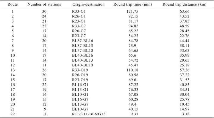
Figure 7 shows the simplified TRTC HCM main line network configuration. The number of stations totals fifty-four, with twenty-two candidate set routes

as shown in Table 2. Table 3 shows five routes and associated headways. Fifty-three trains serve pas-sengers in the timetable. Fig. 8 depicts the headways between end stations. Three segments are very crowded, due to heavy passenger demand during week-day peak hours, in addition to the interchange station BL7/R13 platform. Fig. 8 shows the segments by a solid bold line. Thus the TRTC uses five additional spare trains as shuttle trains to reduce congestion. Nevertheless, if more trains cannot join the opera-tion (because of budget constraints), the crowding problem may worsen, due to growing passenger demand. Moreover, temporarily running shuttle trains is not a good idea from the perspective of auto traffic control. Our network design model provides an al-ternative to solve the problem.

α, β, γ, and λ, in (8), as obtained from operational Table 2 The Candidate route set of case study TRTC HCM main line network

Route Number of stations Origin-destination Round trip time (min) Round trip distance (km)

1 30 R33-G1 121.75 63.66 2 24 R26-G1 92.15 43.52 3 21 R23-G1 81.17 37.83 4 23 R33-G7 94.82 48.59 5 17 R26-G7 65.22 28.45 6 14 R23-G7 54.23 22.76 7 20 BL37-BL16 84.78 44.44 8 17 BL37-BL13 73.9 38.11 9 14 BL37-BL10 64.65 33.63 10 17 BL40-BL16 65.6 35.99 11 14 BL40-BL13 54.72 29.65 12 11 BL40-BL10 45.47 25.18 13 26 R33-O19 110.18 57.36 14 20 R26-O19 80.58 37.22 15 17 R23-O19 69.6 31.53 16 22 BL16-G1 87.22 40.85 17 19 BL13-G1 76.33 34.51 18 16 BL10-G1 67.08 30.04 19 15 BL16-G7 60.28 25.78 20 12 BL13-G7 49.4 19.45 21 9 BL10-G7 40.15 14.97 22 3 R11/G11-BL6/G13 9.33 3.18 R33 R26 R23 BL37 BL6/G13 BL16 R11/G11 G10/O15 O19 G1 BL40 BL7/R13 BL10 BL13 G7

Fig. 7 The HCM main line network structure of TRTC

experience, are 378.8, 1522, 73.8, and 0.00027. The maximum and minimum headways are 7 and 2 minutes, respectively. The population size, number of generations, crossover rate, and mutation rate, as also obtained from experimental tests, are 50, 200, 0.95, and 0.2.

1. Performance Measures Comparison of Initial Solution Generation Methods

This study examines six combinations of two aforementioned initial solution generation methods and three crossover operators (i.e. one-point, one-point mutation, and two-point), in order to compare the performance of initial solution generation methods. Each combination has ten replications and Table 4 describes the results.

The third row of Table 4 illustrates that initial solutions can be generated within a reasonable amount of time. The 4th _{row provides the centralization of}

initial solutions generated by the 1-car method and the minimum-car method. Eq. (28) described below is utilized to compute the variation coefficient on re-lationships between every two initial solutions (x, y) Table 3 The peak-hour route design of TRTC HCM main line network

Route Origin-destination Trains used Headway (min) Train-km Train-hour

1 R33–G1 18 6.76 564.70 18 7 BL37–BL16 12 7.07 377.41 12 10 BL40–BL16 11 5.96 362.09 11 14 R26–O19 11 7.33 304.85 11 22 R11/G11-BL6/G13 1 9.33 20.45 1 Total 53 1629.5 53

Fitness (thousand) 10620.3 Total traveling time 86097.6 hours

3.23 min R11/G11 10 min R33 R26 BL16 BL73 BL6/G13 O19 G01 6.76 min 7.07 min 7.33 min 3.52 min 6.76 min BL40 BL7/R13 G10/O15 Table 4 Comparison of performance measures for initial solution generation methods

Method 1-car Minimum-car

Standard Coefficient of Standard Coefficient of Statistic measures Mean Mean

deviation variation deviation variation Time of generating 109.2 68.6 62.8% 255.7 30.0 11.7% initial solutions (sec)

Coefficient of variation 61.0 2.0 3.3% 61.1 1.2 1.9% on relationships (%)

Computation time (sec) 13099.7 8103.4 61.9% 12287.5 8178.6 66.6% Maximum fitness 4568.4 2125.3 46.5% 3036.4 1416.1 46.6% Fitness of the first 652.5 15.9 2.4% 656.1 11.2 1.7% non-inferior solution

(thousand)

Generation of the first 19 18.8 99.5% 14 14.1 101.5% appearing non-inferior

solution

Fitness of the final solution 623.6 8.7 1.4% 624.8 8.5 1.4% (thousand)

Generation of the first

appearing final solution 71 46.8 66.3% 60 51.2 84.9%

Fig. 8 The peak-hour headway configuration of TRTC MRT net-work

of a replication. Each replication is examined to ob-tain its variation coefficient on relationships. The higher the coefficient, the greater the decentraliza-tion of replicated initial soludecentraliza-tions. Because the coef-ficient means of the 1-car method and minimum-car method are 61.0 and 61.1 separately, the distribution of initial solutions generated by these two methods decentralizes. The best solution is obtained through the genetic algorithm searching strategy.

Relx, y =

Σ

)2 ₍₂₈₎

The other rows of Table 4 compare solution per-formance for these two generation methods. The com-parison result is described below:

(i) The 5th _{row identifies that the minimum-car} method uses less lower computation time. (ii) The 6th _{row describes first generation maximum}

fitness to understand the convergence speed of these two methods. The result shows that the mini-mum-car method is faster then the 1-car method. (iii) The 7th _{and 8}th _{rows describe the fitness and} apparent generation of the first non-inferior so-lutions to identify which method obtains an ac-ceptable solution in a reasonable number of generations. Although the 1-car method gets the lower mean fitness of 652.5 thousands, the gap between the fitness of these two methods is small (656.1 –652.5)/656.1 = 0.6%. The variation co-efficients are 2.4% and 1.7% separately. That is, the values of the first-appearing non-inferior solutions are very close and stable. Besides, the average first-appearing generation of non-infe-rior solutions for the minimum-car method is lower then that of the 1-car method. This result means that the minimum-car method obtains an accept-able solution in fewer generations then the 1-car method.

(iv) The 9th _{and 10}th _{rows describe the fitness and} apparent generation of the first final solutions to identify which method obtains the final solution in a reasonable number of generations. The com-parison result is the same as the non-inferior solution comparison. The values of the first-ap-pearing final solutions are very close and stable. The average first-appearing generation of final solutions of the minimum-car method is lower than that of the 1-car method. This means the minimum-car method obtains a best solution in fewer generations than the 1-car method. (v) To sum up, the values of fitness obtained by the

1-car method and minimum-car method are very close. However, the minimum-car method gets faster convergence speed, uses less computation time, and requires fewer generations to obtain final solutions. It obtains solutions with quality

as well as efficiency, and is suitable for the MTRND problem.

2. Comparison of Performance Measures for Crossover Operators

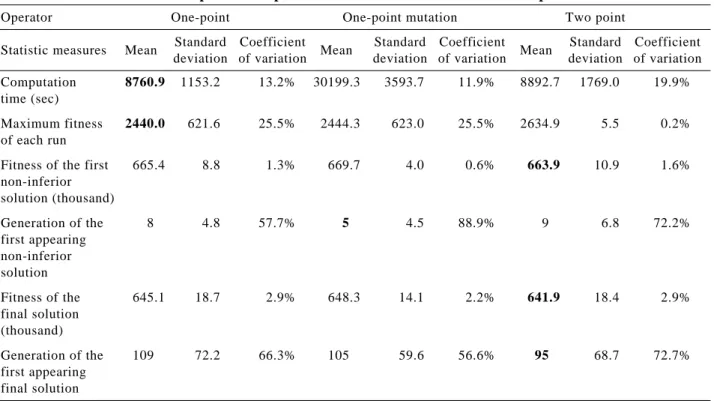
The current work examines the case of the same initial solution generated by minimum-car method by these three crossover operators in order to compare crossover operator performance. Each operator has ten replications, described by Table 5. The result of comparison is described below:

(i) The 3rd _{row identifies that the one-point} muta-tion operator uses the most computamuta-tion time. Computation times of the one-point operator and the two-point operator are very close and com-prise one third of the computation time spent by the one-point mutation operator.

(ii) The 4th _{row identifies that the one-point} opera-tor has the lowest maximum fitness of each run. Convergence speed of this operator is faster than the others.

(iii) The 5th _{row describes that the two-point} opera-tor has the lowest fitness of the first non-infe-rior solutions. The coefficient of variation 1.6% means the quality is stable.

(iv) The 6th _{row identifies that the one-point} muta-tion operator has the lowest first-appearing gen-eration of the first non-inferior solutions. But, computation time for this operator is three times that of the others. The one-point operator and the two-point operator obtain an acceptable so-lution in less time than the one-point mutation operator.

(v) The 7th _{and 8}th _{row identify that the two-point} operator has the lowest fitness and the first-ap-pearing generation of the first final solutions. This means that this operator obtains the best so-lution in fewer generations than the others. (vi) In summary, the values of fitness obtained by the

three crossover operators are very close. Because of less computation time and fewer generations to obtain final solutions, the two-point operator obtains solutions with quality and efficiency, and is suitable for the MTRND problem.

3. Results for Minimum-car Method Plus Two-point Crossover Operator

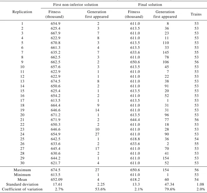
The aforementioned analysis results identify that the combination of the minimum-car method and the two-point crossover operator is suitable for the MTRND problem. This work examines thirty repli-cations in order to understand the hybrid algorithm performance. The result is summarized by Table 6 and described below:

(i) The averaged first appearing generation of the first non-inferior solutions is 4. This means that the big-M application described in Eq. (26) is helpful for algorithm convergence.

(ii) The mass transit system will not be crowded by implementation of these thirty final solutions because their fitness is less than the M. There-fore there is no need for shuttle train manual operation, thus solving the dispatching and crowding problem.

(iii) The averaged first appearing generation of the final solutions is sixty. A designer emphasizing computation time can set the maximum genera-tion to 100 to obtain an acceptable best solugenera-tion. (iv) The maximum, average, and minimum operat-ing trains used by the final solutions are 56, 54, and 53 separately. This verifies that the pro-posed algorithm saves operating trains subject to operational constraints. Reducing operating trains is helpful for saving operation cost and providing residual trains for maintenance purpose. (v) The final solutions are centralized and stable because their coefficient of variation is 2.1%. Eighteen replications get the best solution (fitness = 611.0), which is 60% of the thirty replications. (vi) Six replications get the second best solution (fitness = 613.5), which is 20% of the thirty replications.

(vii) The first two best solutions of the final solutions (fitness = 611.0 and 613.5) are 80% of the thirty replications. This verifies that the proposed

algorithm obtains good solutions robustly. (viii) To sum up, the hybrid algorithm with

minimum-car method and the two-point crossover operator obtains solutions with quality as well as efficiency, and is suitable for the MTRND problem. 4. Discussion of the Best Solution and the Second

Best Solution

Table 7 and Fig. 9 describe the route design and headway configuration of the best solution (fitness = 611.0 thousands) of the thirty replications. Solution characteristics are described below:

(i) The mass transit system will not be crowded and there is no need for the shuttle train. Thus we can dispatch trains automatically and save driver costs. (ii) The number of operating trains is 53, the same as the TRTC. This means that we can leave five spare trains.

(iii) The solution contains three routes. The route configuration is easy for passengers to remember. The minimum headway appears at the CBD. The situation is common for real cases.

(iv) Because the minimum headway of these three routes is 4.31 minutes, when trains arrive at terminal stations, the drivers have sufficient time to walk from the fronts of trains to the rears to continue on to the next trip without the requirement of an extra driver. Thus the driver cost is saved. (v) As per passenger transfer penalty, passengers

from G1 to R33 can change trains to route 13 Table 5 Comparison of performance measures for crossover operators

Operator One-point One-point mutation Two point

Standard Coefficient Standard Coefficient Standard Coefficient Statistic measures Mean Mean Mean

deviation of variation deviation of variation deviation of variation Computation 8760.9 1153.2 13.2% 30199.3 3593.7 11.9% 8892.7 1769.0 19.9% time (sec)

Maximum fitness 2440.0 621.6 25.5% 2444.3 623.0 25.5% 2634.9 5.5 0.2% of each run

Fitness of the first 665.4 8.8 1.3% 669.7 4.0 0.6% 663.9 10.9 1.6% non-inferior solution (thousand) Generation of the 8 4.8 57.7% 5 4.5 88.9% 9 6.8 72.2% first appearing non-inferior solution Fitness of the 645.1 18.7 2.9% 648.3 14.1 2.2% 641.9 18.4 2.9% final solution (thousand) Generation of the 109 72.2 66.3% 105 59.6 56.6% 95 68.7 72.7% first appearing final solution

easily at the G10 or G11 station. The average waiting time is 2.5 minutes (half of the headway of route 13). They needn’t spend too much time transferring in the system.

(vi) As per link capacity, the links between BL6/G13 and BL10 own maximum capacity. The headway

is 2.41 minutes and still exceeds the minimum constraint of 2 minutes. Additional trains can ex-pand the capacity if needed.

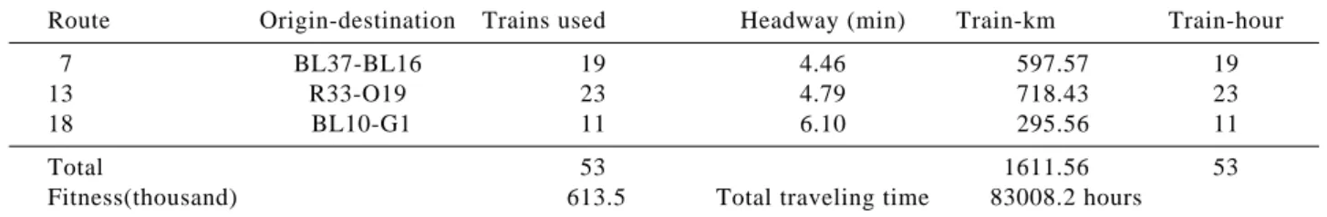
Table 8 and Fig. 10 describe the route design and headway configuration of the second best solu-tion (fitness = 613.5 thousands) of the thirty replicasolu-tions. Table 6 Results for the minimum train method plus two-point crossover operator

First non-inferior solution Final solution Replication Fitness Generation Fitness Generation

Trains (thousand) first appeared (thousand) first appeared

1 654.9 2 611.0 8 53 2 625.4 3 613.5 36 53 3 667.9 7 611.0 23 53 4 622.9 8 611.0 11 53 5 670.8 3 613.5 110 53 6 661.3 4 613.5 33 53 7 635.2 7 633.6 145 55 8 662.5 3 611.0 78 53 9 662.5 2 650.6 106 56 10 657.6 3 613.5 45 53 11 622.9 1 611.0 7 53 12 622.9 1 611.0 22 53 13 674.5 8 611.0 38 53 14 650.6 2 611.0 91 53 15 625.4 1 613.5 20 53 16 654.2 2 611.0 52 53 17 613.5 1 613.5 1 53 18 664.4 9 611.0 31 53 19 646.6 14 611.0 31 53 20 671.2 1 613.5 96 53 21 671.9 2 644.4 77 56 22 650.3 2 611.0 18 53 23 646.6 10 611.0 28 53 24 654.9 27 611.0 90 53 25 642.5 1 618.8 36 54 26 633.6 2 633.6 2 55 27 645.4 17 611.0 70 53 28 630.6 2 611.0 41 53 29 644.2 1 611.0 154 53 30 621.7 4 611.0 52 53 Maximum 674.5 27 650.6 154 56 Minimum 613.5 1 611.0 1 53 Mean 652.09 4 618.2 60 54 Standard deviation 17.61 2.25 13.3 47.34 1.08 Coefficient of variation 2.7% 53.6% 2.1% 79.6% 2.0%

Table 7 Route design of the best solution

Route Origin-destination Trains used Headway (min) Train-km Train-hour

9 BL37-BL10 15 4.31 468.17 15

13 R33-O19 22 5.01 687.20 22

16 BL16-G1 16 5.45 449.62 16

Total 53 1604.99 53

Fitness (thousand) 611.0 Total traveling time 84418.7 hours

Table 8 Route design of the second best solution

Route Origin-destination Trains used Headway (min) Train-km Train-hour

7 BL37-BL16 19 4.46 597.57 19

13 R33-O19 23 4.79 718.43 23

18 BL10-G1 11 6.10 295.56 11

Total 53 1611.56 53

Fitness(thousand) 613.5 Total traveling time 83008.2 hours

Because of good cost, transfer convenience, and route configuration combination, the second best solution is worth considering. The designer can decide which solution is suitable to fit his objectives.

VII. CONCLUSIONS

This paper presents a genetic algorithm to solve the MTRND problem on real mass transit networks. In order to overcome special MTRND problem characteristics, the effects of special genetic coding, an initial feasible solution creating method, network representation, repair strategy, improved fitness function, crossover operators, mutation operator, and redundancy checking are illustrated and applied to avoid infeasible initial solutions, save computation time, and improve solution quality. A detailed analysis is carried out examing real the TRTC network in Taipei. Compari-sons between two initial solution-creating methods and three operators find out whether combining the mini-mum-car method and the two-point crossover operator are suitable for this use. Case study results indicate that the model and the proposed algorithm could be useful for the MTRND problem in the real world.

ACKNOWLEDGMENTS

The authors acknowledge the support of the Taipei Rapid Transit Corporation (TRTC).

NOMENCLATURE

fkrs trips on the kth path of the alternate

paths from the rth station to the sth station

Fi frequency of the ith route in trains/

hour

i the ith route

n number of routes in network

na, nb, nc, nd, ne number of links of type a, b, c, d,

and e accordingly

OT minimum allowable headway of

segments in hours

PT maximum allowable headway of

segments in hours

r the rth origin station

RLi round trip distance of the ith route

in kilometers

RTi round trip time of the ith route in

hours

s the sth destination station

si binary variable that is 1 if the ith

route is chosen; 0 otherwise

Trs trips from the rth station to the sth

station

TRc train capacity in riderships/train

TRC fleet size in trains

TSi trains used by the ith route in trains

xa, xb, xc, xd, xe integer variables that are flow of

link type a, b, c, d, and e accord-ingly in trips

α operating cost per train-km

β depreciation funds per train-hour

γ passenger’s in-vehicle time cost

per hour

λ weight which is decided by designer

Fig. 9 Headway configuration of the best solution 5.45 min 5.01 min R33 BL16 BL37 O19 G01 5.01 min 5.45 min 4.31 min 5.45 min BL10 2.61 min 2.41 min R11/G11 BL6/G13 G10/O15 6.1 min R33 BL16 BL37 O19 G01 4.46 min 4.79 min 6.1 min 4.79 min 4.46 min BL10 2.68 min 2.58 min R11/G11 BL6/G13 G10/O15

Fig. 10 Headway configuration of the second best solution

θij binary variables that are 1 if

seg-ment j is served by the ith route ; 0 otherwise

δrs

ak, δrsbk, δrsck, δrsdk, δrsek binary variables that are 1 if

links of type a, b, c, d, and e are included in the kth route for the rsth O-D; 0 otherwise

va, vb, vc, vd, ve capacity of links of type a, b, c, d,

and e in trips

Za, Zb, Zc, Zd, Ze binary variables that are 1 if the flow

of links of type a, b, c, d, and e ex-ceed their capacity; 0 otherwise; and (r, s) trips from the rth station to the sth

station.

REFERENCES

Agrawal, J., and Tom, V. M., 2004, “Transit Route Net-work Design Using Parallel Genetic Algorithm,”

Journal of Computing in Civil Engineering, Vol. 18,

No. 3, pp. 248-256.

Ben-Ayed, O., Boyce, D. E., and Blair, C. E., 1988, “A General Bi-Level Linear Programming For-mulation of the Network Design Problem,”

Trans-portation Research Part B, Vol. 22, No. 4, pp.

311-318.

Ceder, A., 2003, “Designing Public Transport Net-works and Routes,” Advanced Modeling for Transit

Operations and Service Planning, Lam, W., Bell,

M., Eds., Oxford, UK, Chapter 3, pp. 59-91. Chang, S. K., and Guo, Y. J., 2007, “Development of

Urban Full Trip Cost Models,” Transportation

Planning Journal, Vo1. 36, No. 2, pp. 147-182.

Chiou, S. W., 2005, “Bi-Level Programming for the Continuous Transport Network Design Problem,”

Transportation Research Part B, Vol. 39, No. 4,

pp. 361-383.

Constantin, I., and Florian, M., 1995, “Optimizing Headway in a Transit Network: a Nonlinear Bi-Level Programming Approach,” International

Transactions in Operational Research, Vol. 2,

No. 2, pp. 149-164.

Fan, W., and Machemehl, R., 2004, “Optimal Transit Route Network Design Problem: Algorithms, Im-plementations, and Numerical Results,” Technical

Report SWUTC/04/167244-1, Center for

Transpor-tation Research, University of Texas, USA. Fan, W., and Machemehl, R., 2006a, “Optimal

Tran-sit Route Network Design Problem with Variable Transit Demand: Genetic Algorithm Approach,”

Journal of Transportation Engineering, Vol. 132,

No. 1, pp. 40-51.

Gao, Z., Sun, H., and Shan, L. L., 2004, “A Continu-ous Equilibrium Network Design Model and Al-gorithm for Transit Systems,” Transportation

Research Part B, Vol. 38, No. 3, pp. 235-250.

Gao, Z., Wu, J., and Sun, H., 2005, “Solution Algo-rithm for the Bi-Level Discrete Network Design Problem,” Transportation Research Part B, Vol. 39, No. 6, pp. 479-495.

Goldberg, D. E., 1989, Genetic Algorithms in Search,

Optimisation, and Machine Learning,

Addison-Wesley, Boston, MA, USA.

Guan, J. F., Yang, H., and Wirasinghe, S. C., 2006, “Simultaneous Optimization of Transit Line Con-figuration and Passenger Line Assignment,”

Transportation Research Part B, Vol. 40, Issue

10, pp. 885-902.

Guihaire, V., and Hao, J. K., 2008, “Transit Network Design and Scheduling: A Global Review,”

Transportation Research Part A, Vol. 42, No. 10,

pp. 1251-1273.

Lee, C. K., and Hsieh, W. J., 2002, “A Bilevel Pro-gramming Model for Planning High Speed Rail Service,” Transportation Planning Journal, Vol. 31, No. 1, pp. 95-119.

Sheffi, Y., 1985, Urban Transportation Network, Prentice-Hall, Englewood Cliffs, N.J. USA. Tom, V. M., and Mohan, S., 2003, “Transit Route

Net-work Design Using Frequency Coded Genetic Algorithm,” Journal of Transportation Engineering, Vol. 129, No. 2, pp. 186-195.

Turmquist, M. A., 1978, “A Model for Investigating the Effects of Service Headway and Reliability on Bus Passenger Waiting times,” Transportation

Research Record 663, pp. 70-73.

Wirasinghe, S. C., 2003, “Initial Planning for Urban Transit Systems,” Advanced Modeling for

Tran-sit Operations and Service Planning, Lam, W.,

Bell, M., Eds., Pergamon, Kowloon, HK, Chap-ter 1, pp. 1-29.

Yin, Y., 2000, “Genetic-Algorithm-Based Approach for Bilevel Programming Models,” Journal of

Trans-portation Engineering, Vol. 126, No. 2, pp. 115-120.

Yang, H., Yagar, S., Iida, Y., and Asakura, Y., 1994, “An Algorithm for the Inflow Control Problem on Urban Freeway Networks with User Optimal Flows,” Transportation Research Part B, Vol. 28, No. 2, pp. 123-139.

Zhao, F., and Zeng, X., 2006, “Optimization of Transit Network Layout and Headway with a Combined Genetic Algorithm and Simulated Annealing Method,” Engineering Optimization, Vol. 38, No. 6, pp. 701-722.

Zhao, F., and Zeng, X., 2006a, “Simulated Anneal-ing–Genetic Algorithm for Transit Network Optimization,” Journal of Computing in Civil

En-gineering, Vol. 20, No. 1, pp. 57-68.

Manuscript Received: Dec. 10, 2008 Revision Received: Feb. 28, 2009 and Accepted: Mar. 31, 2009