Performance assessment of processing and delivery times for very large scale integration using process capability indices

Ownership and Copyright

 2002 Springer-Verlag London Limited

Performance Assessment of Processing and Delivery Times for

Very Large Scale Integration Using Process Capability Indices

K. S. Chen

1

_{, H. T. Chen}

2

_{and Lee-Ing Tong}

2

1_{Department of Industrial Engineering and Management, National Chin-Yi Institute of Technology, Taichung, Taiwan;} 2_{Department of}

Industrial Engineering and Management, National Chiao Tung University, Hsinchu, Taiwan

Process quality and delivery time have received increasing attention in the highly competitive electronics industry. Many studies have proposed process capability indices (PCIs) to assess process effectiveness. However, methods to assess the performance in terms of processing and delivery times of products have seldom been discussed. The conventional PCIs can no longer assess the processing time (PT) and delivery time (DT) performance objectively or identify the relationship between PCIs and the non-conformance rate of PT or the conformance rate of DT. Lacking an effective performance index or an objective testing procedure to assess process/product performance will lead to inefficiency or a high manufacturing management overhead cost. Therefore, this study offers effective performance indices (i.e., PCIs) to assess the PT and DT performance for very large scale integration (VLSI). The uniformly minimum variance unbiased (UMVU) estimators of the proposed PCIs are derived under the assumption of a normal process distribution. The PCI estimators are then employed to construct a one-to-one relationship between the PCIs and the conformance rate of DT or non-conformance rate of PT, respectively. Finally, hypothesis testing procedures for the proposed PCIs are also developed. The testing pro-cedure can be used to determine whether DT or PT can satisfy a customer’s requirements.

Keywords: Delivery time; Normal distribution; Process

capa-bility index; Processing time; Uniformly minimum; Variance unbiased estimator; Very large scale integration

1.

Introduction

As the global trends of dividing production work and reducing product life cycles continue, the build to order (BTO) model is gradually replacing the build to forecast (BTF) model, and

Correspondence and offprint requests to: Dr K. S. Chen, National

Chin-Yi Institute of Technology, 35, Lane 215, Sec. 1 Chung Shan Road, Taiping, Taichung, 411 Taiwan. E-mail: kschen@chinyi.nci-t.edu.tw

is being used by direct-sale computer companies such as Dell and Gateway 2000. According to the investigations of Dickson [1] and Weber et al. [2], process quality and delivery time have been increasingly emphasised in the highly competitive electronics industry. Enhancing the quality and yield of the products, to satisfy customers’ requirements, and delivering those products to the customers on time, are becoming the primary factors in enhancing manufacturers’ marketing com-petitiveness. Lacking an effective performance index and a statistical testing procedure to assess process/product perform-ance leads to inefficiency and a high manufacturing manage-ment overhead cost. Furthermore, manufacturers lose their mar-ket competitiveness if they do not perform well in product quality and delivery because the manufacturers’ production schedule is delayed, and the customers’ profits may even be damaged.

Process capability analysis is a convenient and powerful tool for measuring process performance and capability. Hence, process capability indices (PCIs) have been much studied. Many quality engineers and statisticians (e.g. [3–7]) have pro-posed methodologies for assessing product/process quality. Although this work has received considerable attention and related evaluation methods have been developed, the processing time (PT) and delivery time (DT) performance of products/processes has seldom been discussed. The importance of PT and DT of products is increased under the BTO model. Conventional PCIs can no longer assess the PT and DT performance objectively or identify the relationship between PCIs and the non-conformance rate of PT or the conformance rate of DT.

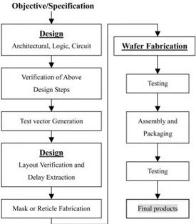
Figure 1 shows the stages from accepting orders to delivering products for the manufacture of very large scale integration (VLSI). These stages can be grouped into two phases: 1 The design phase.

2 The fabrication phase.

In the former, the desired functions and required operating specifications of the circuits are initially decided upon. The chip is then designed from the “top down”. That is, the required large functional blocks are first identified. Next, their sub-blocks are selected, and then the logic gates required to

Fig. 1. Stages required for the manufacture of VLSI.

implement the sub-blocks are chosen. Each logic gate is designed by connecting devices that are ultimately used for fabrication on the wafers. Upon completing these various design levels, each is checked to ensure that correct func-tionality obtains. Then, the layout of the VLSI is recognised. Research and development time (i.e., the design phase) must be reduced for products/processes with a shorter life cycle to increase the market share.

Some physical and chemical technologies are employed in the fabrication of the VLSI. These are used in the oxidation, deposition, implantation, diffusion, evaporation, etc. The chip layout is miniaturised and manufactured on the wafers by sequential photolithography, mask and etching stages [8, 9]. The finished wafers are tested. Conformance chips are assembled, packaged and re-tested. Conforming products are called final products, and are shipped.

The VLSI process includes a design phase and a fabrication phase, each of which can be divided into stages. Each stage may also include several processing steps with similar features. Therefore, the PT of the design phase and each processing stage directly influences the DT of final products. This study offers an efficient hypothetical testing procedure for PCIs, capable of assessing the PT and DT performance of the VLSI. The PCIs of PT and DT are initially defined, and the uniformly minimum variance unbiased (UMVU) estimators of the studied PCIs are derived under the assumption of a normal distribution. The above estimators are then used to construct a the one-to-one relationship between the PCIs and the conformance rate of DT (or the non-conformance rate of PT). Finally, a hypoth-esis testing procedure for PCIs is established. The hypothhypoth-esis testing procedure allows manufacturers to assess the PT per-formance of an individual processing stage for the manufacture of VLSI, and to determine whether the DT performance satis-fies customers’ requirements, thereby increasing the competi-tiveness of suppliers. Corresponding tables of non-conformance rate of PT performance and the conformance rate of DT

performance are also provided to verify the required perform-ance index value for manufacturers.

The rest of this paper is organised as follows. Section 2 defines and introduces the PT and DT performance indices. Section 3 derives the estimators of PT and DT performance indices. Section 4 constructs the practically applicable hypoth-esis-testing procedures. Conclusions are drawn in Section 5.

2.

The PT and DT Performance Indices

This section defines the PT performance index of each stage for processing VLSI. The DT performance index is then given to assess the DT capability of the final products.

2.1 The PT Performance Index (Qi)

PT represents the time of processing a stage for VLSI. Each stage of processing VLSI has a corresponding PT, that directly affects manufacturers’ DTs. Therefore, efficiently monitoring and improving the process is a valuable exercise for manufac-turers. Suppose k stages must be processed in a complete manufacturing process of VLSI to create the final products. Let k stages of processing VLSI have upper time limits, U1,

U2 ,%, Uk (where

冘

k

i=1

UiⱕUT, UT is the upper time limit of DT). Assume that X1, X2, %, Xk represent the actual PTs of

k stages for processing VLSI (perhaps including assembly,

testing stages, and design phase), then T =

冘

k

i=1

Xi is the DT. The unit time may be stated in seconds, minutes, hours, days, or some other unit. Generally, the PT of each stage for processing VLSI varies, such that, X1, X2%, Xkare k normally distributed random variables.

Generally, a shorter PT implies a better performance. Hence, the PT of VLSI exhibits smallest-the-best type quality charac-teristic. Suppose (µ1,σ1),(µ2,σ2),(µk,σk) represent the mean and standard deviation of PT for k stages of processing VLSI, respectively, then the PT performance index of the ith stage can be defined as follows:

Qi=

Ui⫺µi σi

(1) where i = 1,2%,k. The numerator of index Qi, (Ui⫺µi), rep-resents the upper time limit Ui of PT of the ith stage, and differs from the actual mean PT, µi, which is employed to assess the mean performance of the ith PT. Qi and thus the performance of the ith PT, increases with (Ui⫺µi). The denominator of index , Qi,σi, is the standard deviation of the

ith PT. A smallerσindicates a more stable PT at the ith stage and a superior VLSI processing performance, yielding a larger

Qi. Hence, Qi can reasonably reflect the PT performance for the ith stage of processing VLSI.

In practice Xi⭐Ui, is desired, such that the ith PT conforms to the upper specification limit, and the PT of the ith stage is defined as a conformance PT; otherwise, PT is defined as a non-conformance PT (i.e., Xi⬎Ui). The ratio of the non-con-formance PT is known as the non-connon-con-formance rate. Assuming

a normal distribution, the relationship between the non-con-formance rate of the ith PT, Pi, and the index Qi, can be expressed as follows: Pi= Pr(Xi⬎Ui) = 1 ⫺ Pr(Xi⭐Ui) = 1 ⫺ Pr

冉

Xi⫺␮i ␴i ⱕUi⫺␮i ␴i

冊

(2) = 1 ⫺ Pr(Zi⭐Qi) = 1 ⫺ φ(Qi)

where i = 1,2%,k, Zi is a standard normal distribution, and Φ is the cumulative function of the standard normal distribution. Clearly, a larger Qicorresponds to a smaller non-conformance rate of PT, and is a superior process performance. Conse-quently, the PT performance index for k stages adequately reflects the non-conformance rate of each processing stage, and a one-to-one mathematical relationship exists between Qi and non-conformance rate, Pi. Consequently, Table 1 can be used precisely and quickly to estimate the non-conformance rate of PT, Pi using the performance index, Qi.

For instance, Qi = 1 gives Pi = 1⫺Φ(Qi) = 1⫺Φ(1) = 15.86% from Table 1; Qi = 2 gives Pi = 2.28%, and so on. For the Qi values which are not listed in Table 1, the non-conformance rate, Pi, can be determined by interpolation, or by checking a standard normal probability distribution table.

Pican be computed by dividing the non-conformance number of the ith PT by the total sampling number of VLSI. A smaller

Pi requires a larger sample size to estimate precisely its value (see [10] for details). Therefore, using the one-to-one relation-ship between Qi and Pi, the PT (Qi) index can be a very convenient and effective tool not only for evaluating the per-formance of an individual PT, but also for accurately estimating the non-conformance rate, Pi.

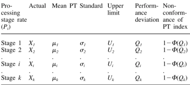
Table 2 summarises the actual PT, mean time, standard deviation time, upper limit of PT, index and corresponding non-conformance rate for k processing stages. The table can be employed not only to assess the performance of the ith PT, but also as a reference for enhancing performance.

As the DT performance proposed in the following subsection is poor, the higher non-conformance rates Pi among k pro-cessing stages are investigated and improved, reducing the non-conformance PTs to meet the target value of DT. Theoretically, the final products can be delivered on time if the k PTs (Xi) for processing VLSI are all less than the corresponding upper

Table 1. Qi = 1.0 (1.0)6.0 vs. Pi.

PT performance index Qi Non-conformance rate of PT, Pi

1.0 0.158655254 2.0 0.022750132 3.0 0.001349898 4.0 0.000031671 5.0 0.000000287 6.0 0.000000001

Table 2. Actual PT, mean time, standard deviation time, upper limit, index and non-conformance rate for k processing stages

Pro- Actual Mean PT Standard Upper Perform-

Non-cessing limit ance

conform-stage rate deviation ance of

(Pi) PT index Stage 1 X1 ␮1 ␴1 U1 Q1 1⫺⌽(Q1) Stage 2 X2 ␮2 ␴2 U2 Q2 1⫺⌽(Q2) . . . . Stage i Xi ␮i ␴i Ui Qi 1⫺⌽(Qi) . . . . Stage k Xk ␮k ␴k Uk Qk 1⫺⌽(Qk) limit Ui. (i.e. T=

冘

k i=1 Xiⱕ

冘

k i=1

Ui⭐UT where UT represents the upper limit of DT).

2.2. The DT Performance Index (QT) The DT T=

冘

k

i=1

Xiis a random variable possessing a normal distribution with mean, ␮ =

冘

k i=1␮ i and variance, ␴2=

冘

k i=1␴

i2 as X1, X2,%,Xk represent the actual PTs for processing k stages of VLSI. A shorter DT corresponds to a superior process performance. That is, DT possesses a so-called smallest-the-best type quality characteristic. For the same reason as mentioned above with respect to the PT performance index, if the upper time limit of DT is UT (i.e., TⱕUT), then the DT performance index, QT can be defined as follows:

QT=

UT⫺␮

␴ (3)

Suppose DT does not exceed UT, then the process is defined as a conformance process. The ratio of the processes con-forming to UT is known as the conformance rate of DT, and can be expressed as

PT=Pr(TⱕUT)=Pr

冉

Zⱕ

UT⫺␮

␴

冊

=⌽(QT) (4)

Equation (4) shows that a one-to-one mathematical relationship exists between QT and PT. Table 3 summarises the DT performance index values for VLSI, QT, versus corresponding conformance rates, PT. If PT is known, QT can be obtained from Table 3. The testing procedure described in Section 4

Table 3. QT= 1.0 (1.0)6.0 vs. PT.

DT performance index QT Conformance rate of DT, PT

1.0 0.841344746 2.0 0.977249868 3.0 0.998650102 4.0 0.999968329 5.0 0.999999713 6.0 0.999999999

can then be used to check whether a manufacturer’s DT performance meets the required target value, QT. For values not listed in Table 3, the conformance rate PT can be obtained by interpolation or can be checked from a standard normal probability distribution table.

A larger QT value corresponds to a higher DT conformance rate, PT. Not only can the DT performance index PT correctly reflect a manufacturer’s ability to deliver on time but it can also evaluate the stability and conformance rate of DT. There-fore, the performance index QT is a rational, convenient, and efficient tool for assessing DT performance of VLSI manufac-turers.

3.

Estimating PT and DT performance

indices

This section describes only the estimation of the DT perform-ance index, since the estimated methods and procedures con-cerning both DT and PT performance indices are the same. Table 4 summarises the estimators.

In practice, the meanµ and standard deviation ␴ of the true DT are unknown. Therefore, a sample of size n is taken to estimate these values. Let Tibe the actual delivery time of the

ith lot of VLSI. (T1,T2,%,Tn) then represents a random sample drawn from a normal population with mean µ and standard deviation σ. Suppose the sample mean T=

冘

n n=1 Ti/n and stan-dard deviation S=

冪

冘

n i=1

(Ti⫺T)2/(n⫺1) are used to estimate the population meanµ and standard deviation σ. The intuitive estimator of the DT performance index, QT, can be expressed as follows:

Q˜T=

UT⫺ T¯

S (5)

Similarly, the intuitive estimator of the PT performance index (Qi) for the ith stage can be written as Q˜i=

Ui⫺X¯i Si ,i=1,2,%,k, where X¯i=

冘

n j=1 Xij/n, S2j=

冘

n j=1 (Xij⫺X¯i)2/(n⫺1).

Assuming a normal population, the expectation of Q˜lis

E(Q˜l)=(A⫺1n )Ql (6) (see Appendix A for details), where l = 1, 2,%,k, T, and

An=

冪

冉

2

n⫺1

冊

⫻

冤

⌫((n⫺1)/2) ⌫((n⫺2)/2)

冥

(n⬎2)

Clearly, An is a function of sample size n and is difficult to compute. Consequently, Bn=

冪

冢

n⫺2 n⫺1

冣冢

1⫺ 1 4(n⫺2)

冣

+

冢

1 32(n⫺2)2

冣

+

冉

5 128(n− 2)3

冊

(n⬎2)

can be employed to approximate An (i.e., An⬵Bn). As n increases, An becomes very close to 1. That is, Q˜l is an approximate unbiased estimator of Ql, implying that, although

Q˜lis a biased estimator of Ql, it can easily be modified to be an unbiased estimator of Ql from Eq. (6) as follows:

Qˆl=An⫻Q˜lwhere l= 1,2,%k,T (7) since An⬍ 1, and Qˆlis an unbiased estimator of Ql. Therefore,

Var (Qˆl)⬍Var (Q˜ˆ l) and MSE (Qˆl)⬍MSE (Q˜ˆ l) can be found, where l = 1, 2,%,k, T. Similarly, for a DT performance index,

QT, QˆT is not only an unbiased estimator of QT (i.e.,

E(QˆT)=QT)), but is also a function of the complete and sufficient statistic T¯,S2_{. Consequently, Qˆ}

T is the best estimator (i.e., UMVU estimator) of QT. For the same reason, Qˆlis the best estimator of Qi for the ith stage of processing VLSI. The variance of Ql can be derived as follows (see Appendix B for details). Var(Qˆl)=

冢

⌫[(n⫺1)/2] ⌫n⫺3)/2] n⫻⌫⫺2[(n⫺2)/2]

冊

(1+nQ 2 l) (8) ⫺Q2 l where l= 1,2,%k,T

Let t⬘ =

冪

Qˆl/An. Then, t is a non-central t distribution with n⫺1 degrees of freedom and a non-central parameter, ␦=

冪

(n)Ql. The probability density function of the best esti-mator of Qˆl can be derived as follows (see Appendix C for details). fQˆ l(x)=

再

A⫺1n ⫻

冪

n⫻2⫺(n/2) ⌫[(n⫺1)/2]

冪

␲(n⫺1)

冎冕

⬁ 0 y

冉

n⫺22

冊

exp

再

(9) ⫺0.5

冋

y+

冉

冪

ny (n⫺1)An x⫺␦

冊

2

册冎

dy where x苸R.

4.

Testing Procedure for PT and DT

Performance Indices

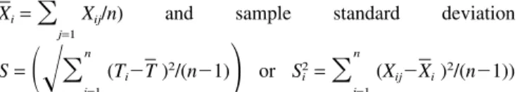
The point estimators of DT and PT performance indices cannot be used directly to determine whether the DT and PT perform-ances of VLSI meet the manufacturer’s requirements, due to sampling error. Thus, a statistical testing procedure is required to assess objectively whether the proposed indices maintain the required values. Assuming that the required DT (or PT) performance index value exceeds or is equal to c, where c is the target value, then the testing procedure for H0:Qlⱕc (the performance index is incapable) vs. Ha:Ql⬍c (the performance index is capable) can be determined, where l = 1, 2,%, k, T. Assuming Ulis known, and using Qˆl, the best estimator of Ql, as the test statistic, then the sample mean T=

冘

n

i=1

Xi=

冘

n

j=1

Xij/n) and sample standard deviation

S=

冉

冪

冘

n i=1 (Ti⫺T )2/(n⫺1)

冣

or S2i =

冘

n j=1 (Xij⫺Xi)2/(n⫺1)) can be calculated from n sample observations. Hence, the estimated value of Qˆl, q, can be obtained. The p-value of the test statistic, Qˆl, can be obtained:

p-value= PR{Qˆl⬎q兩Ql=c}=Pr

再

t⬘⬍

冪

n⫻Q An 兩␦⫺c

冪

n

冎

(10)

t⬘ is a non-central t distribution with n⫺1 degrees of freedom

and a non-central parameter, ␦=c

冪

n in Eq. (10). A statistical

software package, statistical analysis system (SAS), can be used to calculate the p-value= Pr{t⬘⬎T0兩␦=c

冪

n}=1⫺Pr{t⬘⭐

T0兩␦=c

冪

n}=1⫺PROBT (T0;n⫺1;␦=c

冪

n), where T0=(

冪

n⫻

q)/An, and PROBT (T0;n⫺1;␦=c

冪

n), which is lower cumulated

by T0, is the cumulative probability of a non-central t

distri-bution with n⫺1 degrees of freedom and a non-central para-meter, ␦ = c

冪

n in SAS. The p-value can be calculated easily

as c, n and q are known.

The proposed testing procedure can be organised as follows [11] to enable manufacturers to assess conveniently whether the DT or PT performance of VLSI meets the targets.

Step 1. Determine the upper limit of DT or PT, Ul, the performance index value c, and the sample size, n.

Step 2. Specify a significance level, α.

Step 3. Take a sample of size n and calculate the sample mean, and the standard deviation. Using Bn to approximate An, and calculate the value of the test statistic, Qˆl, denoted by q.

Step 4. Determine the p-value using SAS, according to c, q, and sample size, n.

Step 5. Compare the p-value with α. The decision rules are 1. If p-valueⱕα, conclude that the DT or PT performance index meets the target value (or the performance index is capable).

Table 4. The best estimators of PT and DT performance indices

Processing stage PT Sample mean Sample variance Best estimator Q˜_{i Non-conformance Result note}

rate (Pi) Stage 1 X11, X12,%, X1n X1 S12 Qˆ1=An⫻Q˜1 1⫺⌽(Qˆ1) 䊊 Stage 2 X21, X22,%,X2n X2 S22 Qˆ2=An⫻Q˜2 1⫺⌽(Qˆ2) ⫻ . . . . Stage i Xi1, Xi2,%,Xin Xi Si2 Qˆi=An⫻Q˜i 1⫺⌽(Qˆi) ⫻ . . . . Stage k Xk1, Xk2,%,Xkn Xk Sk2 Qˆk=An⫻Q˜k 1⫺⌽(Qˆk) JI DT T1, T2,%,Tn T S2 QˆT=An⫻Q˜T PT=⌽(QˆT) (Conformance rate)

2. If p-value⬎α, conclude that the DT or PT performance index does not meet the target value (or the performance index is incapable).

The DT or PT performance for processing VLSI is assessed easily by using the proposed testing procedure. The following example demonstrates the use of the procedure. Suppose the conformance rate, PT, of DT on time must exceed 97%. Referring to Table 3, a QT value of 2.0 is obtained. Thus, in step 1, the DT performance index is set at c = 2.0. Assume that a sample of size n = 20 is obtained and UT is known. By specifying the significance level, α = 0.01 in step 2, the value, q, of test statistic, QˆT, can be calculated from the sample data in step 3. In step 4, the p-value is obtained using SAS with specified n, c and q. Finally, step 5 compares the p-value with 0.01 and draws a conclusion about the hypothesis. If

p-value⬎α, the true DT performance index meets the required

level, and the performance of DT is satisfactory. Otherwise, the DT performance is unsatisfactory. Table 4 gives the results of the testing procedure for the performance index, Qi , of the

ith PT, and uses the following notation.

The notation ‘䊊’ indicates that the PT of the ith stage for processing VLSI does not exceed the upper limit time, Ui, set by the manufacturers, and that the performance meets the requirement at the ith stage. Otherwise, ‘⫻’ indicates that the PT of the ith stage for processing VLSI, exceeds the upper limit time set by the manufacturers, and the performance does not meet the requirement at the ith stage. In such a case, the manufacturers must assess whether the ith stage delays the DT of VLSI.

5.

Conclusion

This study derives the best estimators of PT and DT perform-ance indices for the manufacture of VLSI, and offers a testing procedure for PT and DT PCIs. The proposed testing procedure can be applied easily by an engineer and can effectively clarify the PT performance for an individual manufacturing stage of VLSI. Additionally, the testing procedure can be employed to assess whether the DT schedule can satisfy the customers, thereby increasing the competitiveness of the suppliers. The corresponding tables of the non-conformance rate of PT are also provided for processing VLSI based on the PT perform-ance indices. The conformperform-ance rate of DT is based on the supplier’s schedule. Hence, for any specified conformance rate,

PT, or non-conformance rate, Pi, a corresponding performance index value, QT or Qi, can be obtained. The proposed testing procedure can also be expressed in terms of the conformance rate.

Acknowledgements

The authors would like to thank the National Council of the Republic of China for financially supporting this research under Contract No. NSC 89-2416-167-006.

References

1. G. W. Dickson, “An analysis of vendor selection systems and decisions”, Journal of Purchasing, 2(1), pp. 5–17, 1996.

2. C. A. Weber, J. R. Current and W. C. Benton, “Vender selection criteria and methods”, European Journal of Operational Research, 50, pp. 2–18, 1991.

3. V. E. Kane, “Process capability indices”, Journal Quality Tech-nology, 18, pp. 41–52, 1986.

4. L. K. Chan, S. W. Chang and F. A. Spiring, “A new measure of process capability: Cpm”, Journal of Quality Technology, 20(3), pp.

162–175, July 1988.

5. R. A. Boyles, “The Taguchi capability index”, Journal of Quality Technology, 23, pp. 17–26, 1991.

6. W. L. Pearn, S. Kotz and N. L. Johnson, “Distributional and inferential properties of process capability indices”, Journal of Quality Technology, 24, pp. 216–231, 1992.

7. K. Va¨nnman, “A unified approach to capability indices”, Statistica. Sinica, 5, pp. 805–820, 1995.

8. S. Wolf and R. N. Tauber, Silicon Processing for the VLSI Era, Process Technology, 2000.

9. C. Mead and L. Conway, Introduction to VLSI Systems, Addison– Wesley, Reading, MA, 1980.

10. D. C. Montgomery, Introduction to Statistical Quality Control, John Wiley, New York, 1985.

11. S. W. Cheng, “Practical implementation of the process capability indices”, Quality Engineering, 7(2), pp. 239–259, 1994.

Appendix A

Q˜T= UT⫺T S =

冪

冉

n⫺1 n

冊

⫻Z⫻C ⫺1 2 where Z=

冪

n(UT⫺T)/␴苲N(

冪

nQT,1), C= (n⫺1)S2/␴2苲␹2n⫺1

Because T¯ and S2_{are mutually independent, so Z and C are also}

independent under the assumption of normal distribution, hence,

E[Q˜T]=

冪

冉

n⫺1 n

冊

⫻E[Z]⫻E[C (⫺1/2)_]=

冪

冉

n⫺1 n

冊

⫻(

冪

n QT) ⫻

冉

⌫[(n⫺2)/2]

冪

2⌫[n⫺1)/2]

冊

=(A⫺1 n )QT Similarly, E[Q˜i]=(A⫺1n )Qi Therefore, E[Q˜l]=(A⫺1n )Qi,l=1,2,%k,T where An=

冪

冉

2 n⫺1

冊

⫻

冋

⌫((n⫺1)/2) ⌫((n⫺2)/2)

册 冉

n⬍2

冊

.

Appendix B

Before deriving the variance of Q˜T, the second moment of

QˆT is derived first, as follows. Because,

Q˜T=An⫻Q˜T=An⫻

冪

冉

n⫺1 n

冊

⫻Z⫻C ⫺1 2 hence, E[Qˆ2 T]=A2n⫻E[Z2]⫻E[C⫺1]⫻

冉

n⫺1 n

冊

= 2 n⫺1 ⫻

冉

⌫[(n⫺1)/2)]_{⌫[(n⫺2)/2)]}

冊

2⫻[1+nQ2_]⫻⌫[(n⫺3)/2)] ⌫[(n⫺1)/2)] ⫻n⫺1 n = ⌫[(n⫺1)/2]⌫[(n⫺3)/2] n⌫2[(n⫺2)/2] ⫻(1+nQ 2 T) Therefore, Var (QˆT)=

冉

⌫[(n⫺1)/2]⌫[(n⫺3)/2] n⫻⌫2[(n⫺2)/2]

冊

(1+nQ 2 T)Q2T Similarly, Var (Qˆl)=

冉

⌫[(n⫺1)/2]⌫[(n⫺3)/2] n⫻⌫2_[(n⫺2)/2]

冊

(1+nQ 2 l)Q2l where l = 1, 2,%,k, T.

Appendix C

QˆT=AnQ˜T=An

冪

冉

n⫺1 n

冊

⫻Z⫻C (⫺1/2)₌An

冑

n⫻T where, T= Z

冪

C/(n⫺1) 苲tn⫺1(␦=

冪

nQT). Let X= Q˜T= An

冪

n ⫻T and there is one-to-one mathematical relationship between X and T, hence, fQ˜ T(x)= fT(t)

|

dT dX

|

= fT

冉

冪

n An x

冊

⫻

冪

n An =fQ˜ i(x) =

再

A -1 n⫻

冪

n⫻2-(n/2) ⌫[(n-1)/2]

冪

␲(n-1)

冎冕

⬁ 0 y

冉

n-22

冊

exp

再

-0.5

冋

y+

冉

冪

ny (n⫺1(An x⫺␦

冊

2

册冎

dy where x苸R.