行政院國家科學委員會專題研究計畫 期中進度報告
十億位元級(Gigabit)無線感知式協同型網路之研究--子計
畫四:Gigabit 無線網路媒體存取控制通信協定之研究
(1/2)
期中進度報告(完整版)
計 畫 類 別 : 整合型 計 畫 編 號 : NSC 96-2219-E-002-027- 執 行 期 間 : 96 年 08 月 01 日至 97 年 07 月 31 日 執 行 單 位 : 國立臺灣大學電信工程學研究所 計 畫 主 持 人 : 謝宏昀 報 告 附 件 : 出席國際會議研究心得報告及發表論文 處 理 方 式 : 本計畫可公開查詢中 華 民 國 97 年 05 月 30 日
Table of Contents
1 Introduction 2
2 Motivation 4
2.1 Experiment Setup 4
2.2 Experiments on Spectrum Utilization 6
2.3 Experiments on Spectrum Sensing – Shadowing 11
2.4 Experiments on Spectrum Sensing – Interference 13
2.5 Summary 15
3 Modeling and Analysis for Cooperative Spectrum Sensing 17
3.1 Related Work 19
3.2 Network Optimization Framework 22
3.3 Numerical Results 27
3.4 Summary 33
4 Building Simulation Platform for Cognitive Radio 33
4.1 The ns-2 PHY and MAC Models 34
4.2 Problems of the ns-2 PHY and MAC Models 39
4.3 Building New PHY and MAC Models 43
4.4 Simulation Results 46
4.5 Summary 49
5 Conclusions and Self Evaluation 50
1 Introduction
One of the greatest challenges facing IEEE 802.11 as it is increasingly used in our daily life is the demand for higher data rate access. The 1997 version of the IEEE 802.11 standard specifies data rates of only 1Mbps and 2Mbps. Over the years, new physical layer technolo-gies have been adopted for increasing the maximum achievable data rates from 11Mbps (802.11b) to 54Mbps (802.11a/g). Despite, several emerging applications have been identi-fied that require substantially higher data rate than that supported by current standards. For example, consumer multimedia applications (e.g. video distributions) in digital home and wireless backhaul connectivity in office buildings require sub-gigabit or even gigabit data rate that is at least an order higher than the maximum data rate supported in IEEE 802.11a/g.
Clearly, the radio frequency spectrum is a scarce resource that does not scale. Most “prime” spectrum nowadays has been assigned, and it is becoming increasingly difficult to find spectrum that can be made available either for new services or to expand existing ones. Demands for the ever increasing data rate by WLAN applications hence should be met by utilizing the spectrum in a more efficient fashion than ever. According to recent studies, some allocated frequency bands are in fact largely unoccupied most of the time - with average occupancy being as low as 10% in some cases. Therefore, if one can explore along the dimension of time by dynamically “filling” these spectrum holes, then it is possible to attain very high data rate without resorting to sophisticated coding or modulation techniques for high spectral efficiency.
From this perspective, the concept of cognitive radio (CR) has come into the limelight. Cognitive radio is a low-cost, highly flexible alternative to the classic single-frequency-band single-protocol wireless device. It is an “intelligent” radio that can perceive its radio envi-ronment through wide-band spectrum sensing techniques and then adapts the transmission or reception parameters such as operating frequency, modulation scheme, code rate, and transmission power in real time. It has been used to improve spectrum sharing so frequency bands allocated to licensed users (primary users) that are rarely used can be accessed by non-licensed users (secondary users) in a “dynamic” and “opportunistic” fashion - as long as the latter yield the channel when needed by the former without introducing interfer-ences. Therefore, a cognitive radio is able to cleverly avoid interference and fill voids in the wireless spectrum, dramatically increasing spectral efficiently.
significant challenges arise when it is intended for WLAN applications requiring sub-gigabit or gigabit data rates. As mentioned before, cognitive radio equipped by secondary users has conventionally been designed to detect the presence of primary users and to yield the channel as soon as possible. The potential data rate degradation due to reduced (or even completely removed) bandwidth usage has not been the primary concern of cognitive radio. However, if cognitive radio is used as the enabling technology for high speed WLAN access, such a complete lack of service assurance (where cognitive radio can potentially be starved indefinitely) could be rather undesirable, especially for applications targeted for multimedia distribution and backhaul connectivity.
In this project, we investigate the problem of using cognitive radio as an enabling technol-ogy for moving the data rate in WLANs to the tune of gigabit per second. In particular, we focus on the design of the MAC layer protocol for such cognitive gigabit wireless networks. Cognitive radio has conventionally been designed to yield the channel when the presence of primary users is detected. However, such a behavior significantly impacts the service provided when it is used as a technology for higher speed WLAN access. We aim to explore along the directions of cognition, cooperation, and coordination for delivering gigabit data service to higher layers.
In the first year, we have made progress along three directions: experiment, modeling, and simulation as follows:
(1) Experiment: We investigate the problems of spectrum utilization and spectrum sens-ing in the frequency bands used by IEEE 802.11a and 802.11b/g. We observe that the spectrum utilization at frequency bands used by 802.11a and 802.11b/g is not very high, and there is much room for cognitive radio technology to be used for leveraging the existence of spectrum holes without significantly decreasing the performance of existing 802.11 users. We also observe through experiments that spectrum sensing (primary transmitter detection) is a non-trivial task, and artifacts such as shadowing and interference will impact the detection probability. More sophisticated spectrum sensing techniques using feature detectors and cooperative detection are needed for cognitive radio users to effectively detect spectrum holes and make use of these spec-trum holes.
(2) Modeling: We investigate the fundamental problems of primary user detection and cooperative spectrum sensing from the perspectives of network optimization. We de-velop a mixed integer non-linear programming (MINLP) model to capture the fun-damental performance difference among different primary transmitter and receiver
BdsE:4E/unq!!!2
BdsE:4E/unq!!!2 311906028!!!¥V¥É!21;21;61311906028!!!¥V¥É!21;21;61
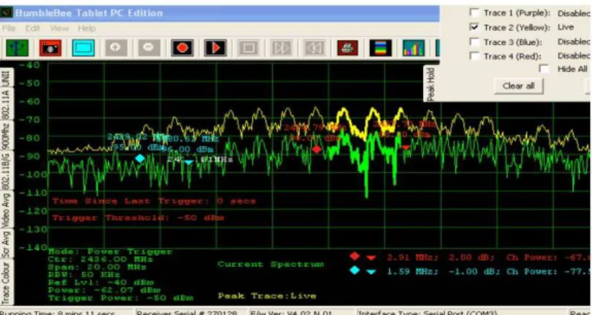
Figure 1. Spectrum Analyzer
detection techniques using energy detection, feature detection, and matched filter detection, as well as using cooperative detection and non-cooperative detection. Nu-merical results based on the proposed optimization framework show the performance tradeoffs of different primary user detection techniques.
(3) Simulation: We move toward building the simulation platform for developing the MAC protocol for cognitive radio networks. Existing ns-2 network simulator does not fully support the accurate simulation in cognitive radio environment, and hence we extend ns-2 to support the functionality of cognition at the physical layer and MAC layer, including calculation of received power and interference, as well as modeling of capture effect and preamble reception.
The rest of the report presents details for the progress that we accomplish in the first year.
2 Motivation
To observe the characteristics of the frequency bands used by 802.11a and 802.11b/g, we measure the spectrum utilization from 5GHz to 5.8GHz (for 802.11a) and from 2.4GHz to 2.5GHz (for 802.11b/g) at different places and times. The following details the experiment setup and the measurement results that we obtain.
2.1 Experiment Setup
We use the Berkeley Varitronics Systems [1] spectrum analyzers for spectrum measurement as shown in Figure 1. The spectrum analyzer on the right is the YellowJacket spectrum analyzer, while the one on the left is the BumbleBee spectrum analyzer.
(a) Spectrum Sweep (b) Persistence Plot Figure 2. Power Spectrum Plot
2.1.1 The YellowJacket Spectrum Analyzer
The YellowJacket spectrum analyzer can be used for spectrum measurement in the fre-quency ranges of 802.11b/g and 802.11a. Measurements of spectrum activity can be per-formed for any subset of channels in the target frequency bands. The power spectrum plot can be used to detect the transmission activities at any particular frequency at any time as shown in Figure 2(a). By recording the instantaneous power level over the target frequency band for a period of time, we can measurement the spectrum usage for further analysis. In addition to instantaneous sweeping of the spectrum, YellowJacket can hold the peak value of the power level at each frequency for N spectrum sweeps as shown in Figure 2(b). The user can change the number of sweeps by adjusting the value in the level entry block for persistence plot.
Figure 3. Histogram Plot
To measurement the spectrum usage over time, Figure 3 can be used. The histogram plot displays the number of occurrences over the last 100 sweeps for power levels at each frequency band that is above the pre-defined power level. The user can adjust the power level through changing the value contained in the histogram level entry block. In the
(a) MAC Level Information (b) Tracking RSSI of an AP Figure 4. Tracking 802.11 AP
histogram plot, the x-axis is the range of frequency bands, while the y-axis is the percentage of time (from 0 to 100) when the power value at each frequency band was above the pre-defined level.
In addition to the power spectrum and histogram plots, the YellowJacket spectrum an-alyzer can also be used to gather information for profiling the operations of the 802.11 protocol. Figure 4(a), for example, shows the MAC level information, including MAC ad-dress, SSID, channel, and RSSI for any particular AP detected in the neighborhood. The RSSI progression versus time for a particular AP can also be traced as shown in Figure 4(b).
2.1.2 The BumbleBee Spectrum Analyzer
The BumbleBee spectrum analyzer is similar in functionality to the YellowJacket spectrum analyzer in spectrum measurement, but it runs on the Tablet PC instead of PDA. It has a frequency control panel that allows the user to set the center frequency and the span of the spectrum analyzer as shown in Figure 5. Up to four traces of the peak power in the live sweep waveform can be set, but only one of these four traces can be active at a given time as shown in Figure 6.
2.2 Experiments on Spectrum Utilization
2.2.1 Experiment Scenario
In the first set of experiment, we measure the spectrum utilization for frequency bands from 5GHz to 5.8GHz (used by IEEE 802.11a) and from 2.4GHz to 2.5GHz (used by IEEE 802.11b/g) in different places and times. Two places on National Taiwan University campus
Figure 5. Frequency Control Panel
Figure 6. Trace of Peak Power Table 1
Time of Day for Spectrum Measurement
morning af ternoon evening
IEEE 802.11b/g at Barry Lam Hall 10:05 to 10:20 13:40 to 13:55 20:00 to 20:15 IEEE 802.11a at Barry Lam Hall 10:25 to 10:40 14:00 to 14:35 20:20 to 20:35 IEEE 802.11b/g at Activity Center 10:10 to 10:25 13:45 to 14:00 20:00 to 20:15 IEEE 802.11a at Activity Center 10:30 to 10:45 14:05 to 14:20 20:20 to 20:35
are chosen for comparison of spectrum utilization: the first place is on the fifth floor of the Barry Lam Hall, and the second place is on the first floor of the Activity Center. It is expected that students will use the wireless network for a longer time and more frequently at the Barry Lam Hall than they are at the open-space Activity Center. For each place, we measure the spectrum usage at different times of the day as shown in Table 1. We show the experiment results in the next section.
0 0.1 0.2 0.3 0.4 0.5 2405 2415 2425 2435 2445 2455 2465 2475 2485 2495 Spectrum Utilization Center Frequency(MHz)
Spectrum Utilization of IEEE802.11b/g in BL Hall morning afternoon evening
Figure 7. Spectrum Utilization of 802.11b/g at Barry Lam Hall
0 0.02 0.04 0.06 0.08 0.1 2405 2415 2425 2435 2445 2455 2465 2475 2485 2495 Spectrum Utilization Center Frequency(MHz)
Spectrum Utilization of IEEE802.11b/g in BL Hall morning afternoon evening
Figure 8. Spectrum Utilization of 802.11b/g at Activity Center
2.2.2 Experiment Results
We divide the frequency bands used by 802.11b/g into ten channels, where the bandwidth of each channel is 10MHz. The spectrum usage for each channel is calculated separately. The spectrum usage of 802.11b/g at the Barry Lam Hall is shown in Figure 7, while that at the Activity Center is shown in Figure 8.
As can be observed from the figures, the spectrum usage at the Barry Lam Hall is much higher than that at the Activity Center. The result is in accordance with our expectation. Residents at the Barry Lam Hall are mostly graduate students, where most of them have
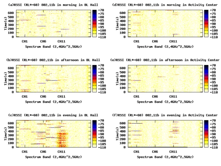
Figure 9. Time-Frequency Plot of Spectrum Utilization
their own notebooks and often use the wireless network for connectivity. Since graduate students typically have their own seats inside the building, they can use the wireless net-work for a longer time. Activity Center, on the contrary, is an open space, where people come and go and use the wireless network, if any, for a relatively short period of time. Regarding spectrum utilization at different times of the day, it can be observed from Figure 7 that the spectrum usage in the morning and afternoon hours is quite similar, but the spectrum usage in the evening is much higher. The reason is that in the daytime most graduate students have to attend the class, but they will come back to their laboratory to conduct research after the evening hours. Therefore, the spectrum utilization in the evening is higher compared to that in the morning and afternoon. Figure 8 shows a slightly different trend, but still the spectrum usage in the evening peaks.
Figure 9 shows the progression of spectrum utilization over time at the Barry Lam Hall and Activity Center at different times of the day. The color of the frequency-time plot shows the strength of the power measured at the particular time slot and frequency band. A blue
0 10 20 30 40 50 2405 2415 2425 2435 2445 2455 2465 2475
Average Spectrum Hole (s)
Center Frequency(MHz)
Average Spectrum Hole of IEEE802.11b/g in BL Hall morning afternoon evening
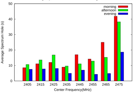
Figure 10. Average Duration of Spectrum Holes (Barry Lam Hall)
or black color denotes that the spectrum is occupied, while a yellow or white color denotes that the spectrum is not used (“spectrum hole”) at the time and frequency measured. It can be observed that the evening spectrum is more occupied compared to the morning and afternoon spectrum as shown in Figures 9(c) and 9(f).
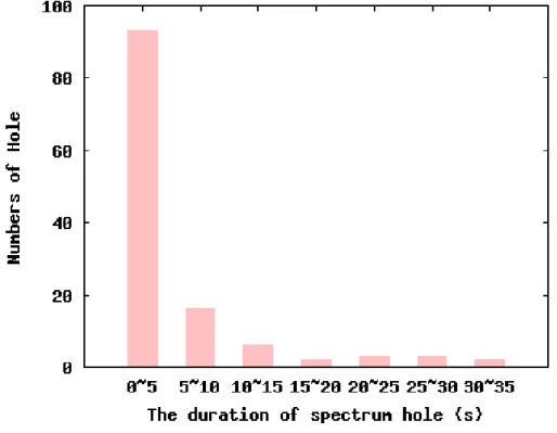
To investigate the distribution of spectrum holes in the ISM band in more depth, we plot the average duration of spectrum holes at the Barry Lam Hall and Activity Center in Figure 10 and Figure 11 respectively. It can be observed that the average duration of spectrum holes at the Barry Lam Hall ranges from about 4s to 40s. The duration of spectrum holes at the Activity Center is longer since the spectrum utilization is much lower. Note that in Figure 11 the average duration of spectrum holes at the 2425MHz and 2435MHz is defined as infinite since no one use these spectrum band at the times of measurement. If we plot the histogram of the duration of spectrum holes from 2.46GHz to 2.47GHz at the Barry Lam Hall in the evening, we have Figure 12. We can observe that the duration of most of the spectrum holes is in the range of zero to five seconds.
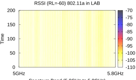
Finally, we show the spectrum usage for the 802.11a frequency band. As shown from the RSSI plot in Figure 13, the spectrum is essentially idle compared to the 802.11b/g band. The result explains the fact that people rarely use 802.11a for connectivity if 802.11b/g is available. Since the 802.11a frequency band ie essentially clear, it can be used for cognitive radio technology in an opportunistic fashion.
0 50 100 150 200 250 300 350 400 2405 2415 2425 2435 2445 2455 2465 2475
Average Spectrum Hole (s)
Center Frequency(MHz)
Average Spectrum Hole of IEEE802.11b/g in Activity Center morning afternoon evening
Figure 11. Average Duration of Spectrum Holes (Activity Center)
Figure 12. Distribution of Spectrum Hole Duration (2.46-2.47GHz; Barry Lam Hall; Evening)
2.3 Experiments on Spectrum Sensing – Shadowing
In primary transmitter detection, the existence and the location of the primary users are unknown to secondary users with cognitive radio. A cognitive radio user therefore can rely on only its local observations based on the weak primary transmitter signals that it receives. In most cases, however, a cognitive radio network is physically separated from the
-110 -105 -100 -95 -90 -85 -80 -75 -70 RSSI (RL=-60) 802.11a in LAB
5GHz 5.8GHz Spectrum Band (5.0GHz to 5.8GHz) 0 50 100 150 200 Time
Figure 13. RSSI Distribution at Barry Lam Hall
primary network and there is no physical or logical interaction between the two networks. It is challenging in this case to design effective and reliable primary user detection techniques by cognitive radio users.
2.3.1 Experiment Scenario
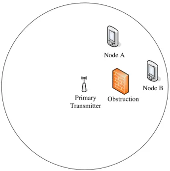
To investigate the problem of primary transmitter user detection due to lack of coordination between cognitive radio users, we design an experiment scenario as shown in Figure 14. Let node A and node B be cognitive radio users that try to detect the presence of the primary transmitter. While node A has line-of-sight communication with the primary transmitter, this is not the case for node B. Hence, node B may not be able to detect the primary transmitter due to the shadowing of the obstruction as shown in Figure 14. We show in the following how this hidden terminal problem impacts the performance of spectrum sensing in cognitive radio networks.
2.3.2 Experiment Results
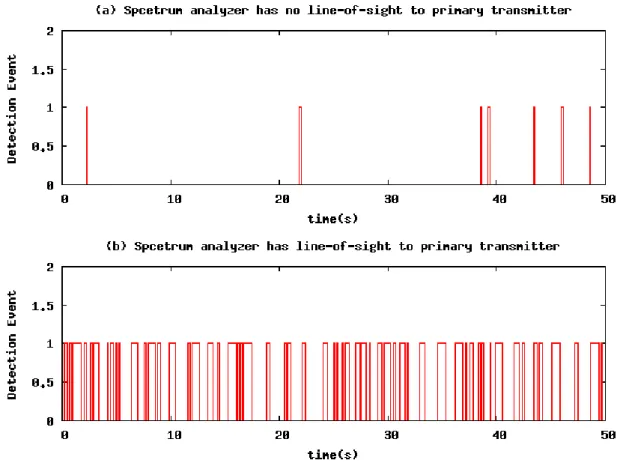
Figure 15 shows the occurrences of detection events at node A and node B when the primary transmitter is constantly beacons to its neighborhood. The y-axis is detection event, where a value of one means that the spectrum analyzer detects the presence of the primary transmitter, and a value of zero means that the spectrum analyzer does not detect any usage of the spectrum band. It is clear from the figure that node B misses many primary user transmission events compared to node A with line-of-sight to the transmitter.
Primary Transmitter
Obstruction Node B Node A
Figure 14. Shadowing Experiment
If node B performs primary transmitter detection alone with assistance from other cognitive radio users, it is expected that the detection performance will be low. A better solution is for node A and node B to cooperate by sharing information from their local observations, and make decisions of spectrum usage after proper fusing of the collected information. For example, if node B in Figure 15 combines the detection information from node A, it can salvage the errors due to obstruction and shadowing. We thus motivate a cooperative technique that can improve the performance and robustness of spectrum sensing.
2.4 Experiments on Spectrum Sensing – Interference
The frequency band used by IEEE802.11b/g is the ISM band from 2.4GHz to 2.5GHz. Many devices have been designed to use the same ISM band such as bluetooth devices, ZigBee devices, microwave ovens, and wireless USB. Energy detector is the simplest ap-proach to perform transmitter detection, but it has a severe disadvantage as being unable to differentiate between different modulated signals, noise and interference. If some devices, not IEEE802.11b/g users, use this frequency band, spectrum sensing based on energy de-tection might mistake them for IEEE802.11b/g users, thus resulting in efficient spectrum sensing by cognitive radio devices. In the following, we design experiments to investigate this problem.
Figure 15. Detection of the Primary Transmitter
2.4.1 Experiment Scenario
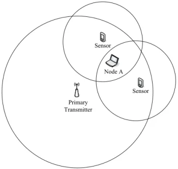
In this experiment, we introduce two TelosB sensor nodes [2] near the spectrum analyzer as interference sources as showed in Figure 16. The sensor nodes operate in the ISM band using IEEE 802.15.4 radio. We increase the number of sensors from 0 to 2 and observe the impact on the detection probability at the spectrum analyzer. We compare the occurrences of detection events for different number of sensors.
2.4.2 Experiment Results
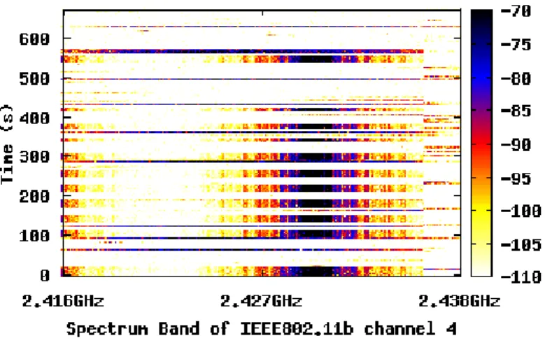
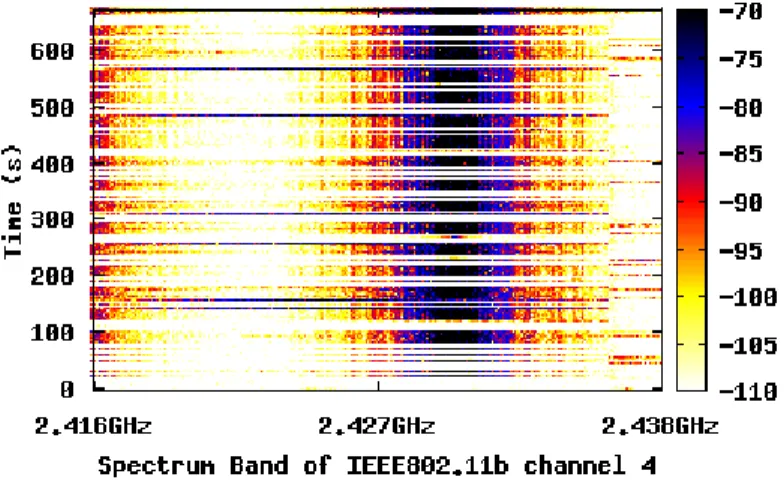
The experiment result is shown in Figure 17. It can be observed that the energy detector (spectrum analyzer) will make make erroneous decisions regarding the transmission events of IEEE 802.11b/g nodes when sensor nodes are around. The count of erroneous decisions increases when the number of sensor nodes increases. The power distribution over time and frequency when the number of sensors is 0, 1, and 2 is shown in Figure 18, Figure 19, and Figure 20 respectively. The interference of sensor nodes can be clearly observed from the figures. One solution to address this problem is to use a more sophisticated detection techniques such as matched filter detection or cyclosationary feature detection.
Primary Transmitter
Node A Sensor
Sensor
Figure 16. Interference Experiment
Figure 17. Detection Event in Presence of Interference
2.5 Summary
To summarize, from the first experiment we observed that spectrum usage varies across different places and different times of the day. The frequency band used by 802.11b/g
Figure 18. Power Distribution with no Sensor Nodes
Figure 19. Power Distribution with One Sensor Node
shows a higher degree of utilization compared to the case of 802.11a. However, in the 802.11b/g frequency band there are still many spectrum holes of significant durations that can potentially be used by secondary users. In the second experiment, we observed the issue with primary transmitter detection. If an energy detector is used for primary user detection and the secondary user does not have line-of-sight to primary transmitters, the detection performance may be low and unreliable. Cooperative spectrum sensing becomes an effective approach to address this problem. In the third experiment, we observed the issue with a simple detector based on energy detection. The ability for the energy detector to detect the presence of primary transmitters degrades as the number of interference sources increases. More sophisticated detector such as matched filter detector and cyclostationary detector can be used to address this problem. In the following, we present how we model the problem
Figure 20. Power Distribution with Two Sensor Nodes
of primary user detection for analyzing and profiling the fundamental performance benefit of cooperative spectrum sensing.
3 Modeling and Analysis for Cooperative Spectrum Sensing
As we observed from the experiment results, a key enabler of the cognitive radio technology is the detection of the spectrum holes (i.e., absence of primary users) through spectrum sensing. As secondary users (CR nodes) may not have accurate knowledge about the whole spectrum at all times, techniques for detecting primary users (PR nodes) need to be em-ployed before spectrum access. Due to the problem of channel fading/shadowing and the existence of hidden terminals, however, detection of primary users based purely on local observation of each CR node may result in poor detection performance.
A conceivable approach therefore is for a group of CR nodes to cooperate and the concerned CR node incorporates information from other CR nodes, instead of completely relying on local observation, for a more accurate detection of primary users. Related work has proposed architecture and network protocols for collaborative sensing in cognitive radio networks using centralized or distributed approaches [3–5]. In centralized approaches, a central control entity is required to gather all sensing information from participating CR nodes through the common control channel. In distributed approaches, on the other hand, CR nodes self-organize to exchange information using local common channels through distributed coordination. Several techniques for optimal fusion of local observations have been proposed in related work [6].
While cognitive radio is a promising technology for maximizing spectrum utilization, there are still many problems to be overcome before it becomes a reality. An objective evaluation and comparison on the capabilities and limitations of different primary user detection techniques, for example, is yet to be investigated due to the lack of well-established hardware
and software platforms for performance evaluation. In this section, instead of jumping
into proposing network architecture and protocols for detecting primary users, we aim to proposed a unified framework to model different primary user detection techniques for better understanding of the fundamental capabilities, limitations, and performance tradeoffs of existing detection techniques. We consider an approach based on network optimization for an objective evaluation of different techniques without being limited by existing software and hardware platforms for cognitive radio technology.
Several studies do exist in the literature that use the approach of network optimization to investigate the capabilities of software defined radio (SDR) or cognitive radio (CR) networks. For example, the authors in [7] investigate spectrum sharing in multi-hop SDR networks. They consider spectrum sensing with sub-band division, scheduling, interference, and flow routing constraints, and then formulate the problem to minimize the total radio bandwidth used in cognitive radio networks. In [8], the authors formulate an optimization problem by jointly considering power control, scheduling, and flow routing constraints in multi-hop SDR networks. The objective is to minimize the bandwidth-footprint product (BFP)in a SDR network. While these studies pave the foundation of our work, the goals are different, and hence the optimization problem of primary user detection for spectrum sharing remains to be addressed.
To proceed, we start by characterizing and comparing different primary transmitter detec-tion techniques, and identify several dimensions for designing primary transmitter detecdetec-tion techniques in cognitive radio networks, including energy detection vs. feature detection, transmitter-side vs. receiver-side detection, and collaborative vs. non-collaborative detec-tion. We then formulate primary transmitter detection techniques along these dimensions using mixed-integer nonlinear programming (MINLP). A formulation for modeling primary receiver detection techniques based on the concept of interference temperature is also pro-posed. We present numerical results based on the proposed optimization framework to show the performance tradeoffs of different primary user detection techniques. We discuss the results with the goal to provide solution perspectives for addressing the problem in future work.
3.1 Related Work
In this section, we categorize related work on primary transmitter/receiver detection into non-collaborative and collaborative detection. We then describe related work based on network optimization that addresses different problems in cognitive radio networks.
3.1.1 Primary Transmitter Detection
The process of detecting primary transmitters starts by classifying and determining the signal from primary transmitters based on local measurements of CR nodes. Several re-lated work has been proposed for detecting primary transmitters [3–5, 9, 10]. Detection of signals from primary transmitters through matched filter detection, energy detection, and cyclostationary feature detection has in particular attracted attention and under in-vestigation by many research endeavors [9–11]. Depending on how local observations are processed in the detection hypothesis model, primary transmitter detection techniques can be categorized into non-collaborative and collaborative detection as discussed in the following:
Non-Collaborative Detection Non-collaborative detection of primary transmitters [9] refers to the case where spectrum sensing information is measured and maintained by individual CR nodes alone to determine the presence of primary transmitters. Local ob-servations based on matched filter detection, energy detection, or cyclostationary feature detection are used without exchanging information with other CR nodes. Since these tech-niques are based entirely on the local observation of a CR node, the problem of hidden terminals due to channel shadowing or insufficient information cannot be avoided.
Collaborative Detection Collaborative detection [3–5] refers to the case where in-formation from multiple CR nodes are incorporated for detecting primary transmitters. Exchange of local observations from individual CR nodes can be implemented either in a centralized or distributed manner [3, 4]. In centralized approaches, a central control entity is required to gather all sensing information from CR nodes through the common control channel. In distributed approaches, on the other hand, CR nodes self-organize to exchange information using local common channels through distributed coordination.
3.1.2 Primary Receiver Detection
In fact, the interference is affected on the primary receiver side, transmitter-based de-tection can not reflect the actual interference. Therefore, FCC defined the interference temperature model [12] to provide a metric that measures the interference experienced by primary receivers. Before classifying the detection techniques, we first describe the in-terference temperature model, and then we describe the primary receiver detection with non-collaborative and collaborative detection.
Interference Temperature Model The interference temperature model manages in-terference at the receiver through the inin-terference temperature limit, which is represented by the amount of new interference that the receiver could tolerate. In other words, the in-terference temperature model accounts for the cumulative RF energy from multiple trans-mission and sets a maximum cap on their aggregate level. As long as CR users do not exceed this limit by their transmissions, they can use this spectrum band. [11] Specifically, a CR user u can access channel A without interfering with primary receiver v only if
IA
v < PuvA − thAv − NA (1)
where IA
v denotes the interference at primary receiver v on channel A, Puv denotes the
received power at v from CR transmitter u, thA
v denotes the interference limit that primary
receiver v can tolerate, and NA denotes the noise level.
Non-Collaborative Detection Non-collaborative detection of primary receivers refers to the case where spectrum sensing information is measured and maintained by individual CR nodes alone to determine the interference level of primary receivers within specific short range. There are some studies investigated the model and characterized the capacity based on interference temperature model [11,13–16]. In [16], they propose a receiver-centric con-straint model for interference temperature metric. In [17], the authors formalize the ideal model and generalized model of interference temperature model. In [17, 18], the authors discussed some practical issues and solutions while implementing the primary receiver de-tection.
Collaborative Detection For collaborative detection, we refer to the case where infor-mation from multiple CR nodes are incorporated for detecting primary receivers. However, there are a few studies to discuss the collaborative primary receiver detection.
CR Transmitter Primary Transmitter r
r
CR Receiver Primary Receiver
Figure 21. Network Scenario
3.1.3 Network Optimization
Several studies exist in the literature that use the approach of network optimization to in-vestigate the capabilities of software defined radio (SDR) networks or cognitive radio (CR) networks. For example, the authors in [7] investigate spectrum sharing in multi-hop SDR networks. They consider spectrum sensing with sub-band division, scheduling, interference constraints, and flow routing, and then formulate the problem of minimizing the total ra-dio bandwidth used in cognitive rara-dio networks as mixed integer non-linear programming (MINLP). In [19], the authors propose a spectrum auction framework for spectrum alloca-tion with interference constraints to maximize aucalloca-tion revenue and spectrum utilizaalloca-tion. In [8], the authors formulate an optimization problem by jointly considering power control, scheduling, and flow routing constraints in multi-hop SDR networks. The objective is to minimize the bandwidth-footprint product (BFP), which characterizes the spectrum and space occupancy for a SDR network.
While these studies pave the foundation of our work, they do not consider the optimization problem of primary transmitter detection for spectrum sharing. We discuss in the follow-ing how we characterize the capabilities and limitations of different primary transmitter detection techniques in cellular cognitive radio networks.
Table 2
Primary User Detection Models
Model Participating Entities A Transmitter only B Receiver only
C Transmitter and receiver
D Transmitter and its neighbors within range r E Receiver and its neighbors within range r
F Transmitter, receiver and their neighbors within range r
3.2 Network Optimization Framework
We consider a network with |Vcr| cells of CR nodes and |Vpr| cells of primary nodes
dis-tributed in the same region as illustrated in Figure 21. In a CR cell, CR users communicate with the CR base station for utilizing spectrum holes left by primary users. We assume that transmission parameters (e.g. transmission powers and operating channels) of individual primary users have already been decided through external mechanisms in absence of the CR users. Transmission parameters of individual CR users, on the other hand, are to be determined by solving the network optimization problem that we present in this section. We formulate the constraints for spectrum sharing among CR and primary nodes from two aspects: CR spectrum sharing and primary user detection. The CR spectrum shar-ing constraint ensures that network resource is shared properly among neighborshar-ing CR users either in the same cell or across different cells. The primary user detection constraint ensures that CR users maximize spectrum utilization while following the primary user detection technique in consideration. We consider both transmitter-centric detection and receiver-centric detection techniques in this report. In the following, we first describe vari-ous primary transmitter detection models that we consider in this report, and then present constraints for CR spectrum sharing and primary user detection.
3.2.1 Detection Models
As shown in Table 2, we compare 6 different detection techniques (models) in this report. Model A refers to the technique where the CR transmitter performs detection based only on its local observation. Model D, on the other hand, involves the transmitter as well as its collaborators. We introduce the parameter r to model the degree of collaboration
exhibited by different detection techniques. Model C can also be considered as a form of collaboration, where both the CR transmitter and receiver are involved to detect the primary transmitter.
To model these different techniques in one framework, we introduce Uuv as the set of CR
nodes that collaborate to detect primary transmitters before communication between the CR pair {uv} takes place. For example, Uuv= {u} for Model A since only the transmitter
u of the pair {uv} is involved to detect primary transmitters. For Model D, the set Uuv
includes the transmitter u and its neighbors within the circle of radius r. Therefore, through proper setting of the set Uuv, it can be used to represent different primary user detection
techniques considered in this report.
3.2.2 CR Spectrum Sharing Constraint
Intra-Cell Constraint We first consider spectrum sharing in a single CR cell (i.e., one serving CR BS and corresponding CR users). We use s(q) to denote the base station for a CR cell with index q ∈ Vcr, and we assume that spectrum available in the cell consists
of a set of |M| unequal-sized frequency bands. If the kth channel is used by node u for
communication with its serving BS s(q), then Xk
us(q) = 1; otherwise, Xus(q)k = 0. We assume
that a communication between a CR user u and its serving base station s(q) is successful if no other users within the same cell are simultaneously transmitting in the same channel. In other words, we assume that a BS can communicate with multiple CR users in different channels, but not if the channels overlap. The interference constraint within a single CR cell thus can be formulated as Equation (5), where CR(q) denotes the CR users within CR cell q excluding BS s(q).
Inter-Cell Constraint We use the physical interference model to determine whether a CR user u can use a spectrum hole k if there exist multiple CR cells in the network. Denote
Pk
uv as the received power at node v on channel k from the signal transmitted by node u
with power Pu. We use the log-normal shadowing model for modeling the propagation gain
from node u to node v as follows: " Pk uv(duv) Pu # dB = K − 10ζ log d0− 10η log à duv d0 ! + XG (2)
where d0 is a close-in distance, duvis the distance between nodes u and v, XG is a Gaussian
random variable with zero mean and standard deviation σG, and K is a constant accounting
path loss exponent up to the close-in distance d0 is denoted as ζ, whereas that beyond is
η.
We assume that a transmission from node u to v is successful only if the SINR at receiver
v exceeds the receiving threshold ∆. Denote Pu as node u’s transmission power, then
transmission from node u to node v on channel k is successful if and only if
Pk uv
N + X
w∈V0
Pwvk ≥ ∆ (3)
where N is the background noise, V0 is the set of nodes that are transmitting
simultane-ously on channel k, and ∆ is a parameter that depends on the desired data rate and the modulation scheme. We thus formulate the interference constraint as Equation (6), where
Vt
pr denotes the set of all primary transmitters and Xwk is a parameter that denotes whether
primary transmitter w transmits on channel k or not.
3.2.3 Primary User Detection Constraint
Transmitter-Centric Constraint As shown in Table 2, we consider different primary transmitter detection models based on the set of participating entities (observers) involved. Note that the signal received by each observer consists of three components including signal from CR transmitters, signal from primary transmitters and background noise. Different signal classification techniques such as matched filter detection, energy detection, and cyclostationary feature detection have been proposed in related work for detecting the presence of primary signals. In this report, we introduce three parameters α, β and γ to model the capability of different detectors in separating the three components from the received signal. For example, an energy detector that simply measures the energy of the received signal has α = 1, β = 1 and γ = 1 since the detector does not distinguish the signal of primary users from that of CR users. If a CR node can perfectly distinguish the signal of primary users from other signal (e.g. through the use of the pilot signal), then
α = 1, β = 0 and γ = 1.
Note that the pair of us(q) in a cell q cannot be active if the presence of primary users is detected. In other words, u can use the channel k if and only if no one in Uus(q) detects the
presence of primary transmitters. We thus formulate the constraint for different primary transmitter detection models as listed in Table 2 using Equation (7).
Maximize X q∈Vcr X u∈CR(q) X k∈M BWklog2 1 + Pus(q)k Xus(q)k N + X i∈Vcr X w∈CR(i)\{u} Pws(q)k Xws(i)k + X w∈Vt pr Pws(q)k Xwk (4) Subject to: X v∈CR(q) Xvs(q)k ≤ 1, ∀k ∈ M, q ∈ Vcr (5) Pk us(q)Xus(q)k N + X i∈Vcr X w∈CR(i)\{u} Pws(q)k Xws(i)k + X w∈Vt pr Pws(q)k Xwk ≥ ∆X k us(q), ∀k ∈ M, u ∈ CR(q), q ∈ Vcr (6) α X w∈Vt pr Pwpk Xwk + β X i∈Vcr X w∈CR(i)\{u} Pwpk Xws(i)k + γN Xk us(q) ≤ ΘXus(q)k , ∀k ∈ M, p ∈ Uus(q), u ∈ CR(q), q ∈ Vcr (7) δ Pk uw+ θ X i∈Vcr X z∈CR(i)\{u} Pk zwXzs(i)k + X v∈Vt pr\{t(w)} Pk vwXvk Xk us(q)Xt(w)k ≤ Ã φ Pk t(w)w − Ωkw ! Xus(q)k Xt(w)k , ∀k ∈ M, w ∈ Eu, u ∈ CR(q), q ∈ Vcr (8)
Receiver-Centric Constraint For receiver-centric primary user detection techniques, the goal is to ensure that the interference incurred by CR transmitters does not exceed the tolerable threshold of interference on primary receivers. If the interference temperature at the primary receiver can be estimated accurately, spectrum sharing between CR nodes and PR nodes can be optimally achieved. Different techniques differ in how the interference temperature at the primary receiver is estimated by a set of collaborating CR nodes and/or sensors. In this report, we model the capabilities of different receiver-centric primary user detection techniques using three parameters: δ, θ, and φ. As Equation (8) shows, δ, θ, and φ models whether a CR node is able to accurately estimate its interference, existing interference at a primary receiver, and desired received power respectively at a primary re-ceiver. For techniques that directly estimate the allowable interference margin at a primary receiver, θ and φ can be lumped together into one parameter. For an ideal primary receiver detection technique, δ = θ = φ = 1. To model the capabilities of different techniques to protect primary receivers, we introduce the parameter Eu. Related work has investigated
different sets of Eu including the primary receivers in the protection region of a primary
200 250 300 350 400 200 250 300 350 400 Y-Axis (m) X-Axis (m) PR TX PR RX CR BS CR User 0 1 2 3 4 5 6 7 8 9 10 11 12 13 14 15 16 17 18 19 20 21 22 23
Figure 22. Simulation Scenario
3.2.4 Objective Function
We consider an objective function that maximizes the total CR throughput (capacity) subject to the aforementioned constraints as follows:
X q∈Vcr X u∈CR(q) X k∈M Ck us(q) (9)
where the link capacity is calculated based on Shannon’s theorem using the following equation: Ck uv= BWklog2 Ã 1 + SIN R ! = BWklog2 1 + Puvk N + X w∈V0 Pk wv (10)
Overall, the objective function together with different constraints for modeling spectrum sharing and primary user detection in cognitive radio networks can be formulated as a mixed-integer nonlinear programming problem. Table 3 lists the symbols used in the for-mulation.
Table 3
Index of Symbols used in the Formulation Symbols Definition
Vcr set of CR cells
Vpr set of primary cells
Vt
pr set of primary transmitters
Uuv set of collaborative CR users for pair {uv}
s(q) base station for a CR cell with index q ∈ Vcr
Xk
us(q) whether link {us(q)} on channel k is active or not
Xk
w whether node w transmits on channel k or not
CR(q) CR users (not including BS) in CR cell q
Pk
uv received power at node v on channel k of the signal transmitted by node u
duv distance between nodes u and v
Pu transmission power of node u
Ck
uv capacity of link {uv} on channel k
BWk bandwidth of channel k N background noise M set of channels ∆ SINR threshold Θ detection threshold Ωk
w allowable interference threshold for receiver w on channel k
t(w) primary transmitter to its receiver w
Eu set of primary receivers protected by node u
3.3 Numerical Results
3.3.1 Results for Primary Transmitter Detection
In this section, we present numerical results to compare the performance of different pri-mary transmitter detection techniques using the proposed optimization framework. The MINLP formulation as shown in Section 3.2 is solved through the NEOS optimization server [20].
Topology and Parameters Setting We consider a network scenario consisting of five primary cells and two CR cells as shown in Figure 22. A CR cell includes one CR base sta-tion and several CR users, whereas a primary cell has an active pair of primary transmitter and receiver. Capacity of each link is determined based on the SINR at the receiver using
Equation (10). The transmission power of each primary transmitter is set to 10 units, and the maximum transmission power of CR transmitters is limited to 50 units. (Note that the actual transmission power of each CR transmitter is to be determined by the optimization
problem.) We assume that the channel bandwidth BWk = 50 for each channel. We vary
the range of collaboration r and detection threshold Θ and observe the performance of each detection technique in terms of interference at primary transmitters.
0 0.005 0.01 0.015 0.02 0.025 0.03 0.035 0.04 0 10 20 30 40 50 60 Interference at Pr Tx r A B C D E F
(a) Energy Detector (Θ = 0.08)
0 0.005 0.01 0.015 0.02 0.025 0.03 0.035 0.04 0 10 20 30 40 50 60 Interference at Pr Tx r A B C D E F (b) Feature Detector (Θ = 0.016)
Results and Discussion We consider both the energy detector and feature detector for detection of primary transmitters, with the former using α = β = γ = 1 and the latter using α = γ = 1 and β = 0. Note that the objective function of the optimization problem is to maximize the CR throughput while following the primary transmitter detection con-straints. To compare the performance of each primary transmitter detection model as we showed in Table 2, we measure the average interference incurred at primary transmitters caused by CR users in the network.
In Figure 23, we vary the range of collaboration r and observe the performance of differ-ent primary transmitter detection models. As shown in Figure 23(a), Models A, B, and C involve only the CR transmitter and/or the receiver, and hence their performance is insensitive to the collaboration range r. Models D, E, and F, on the other hand, involve neighbors within the collaboration range, and hence as r increases (more participating entities for detecting primary transmitters), their interference on primary transmitters is reduced. It can also be observed from Figure 23(a) that the transmitter based model (Model A) incurs slightly higher interference than the receiver based model (Model B). The reason is because the CR receiver (CR base station) can potentially receive from multi-ple CR transmitters (CR users). Since the energy detector cannot separate primary signals from CR signals, the receiver based model will be more conservative in allowing concurrent transmissions from multiple CR transmitters than the transmitter based model. Therefore, the receiver based model can incur lower interference on primary transmitters. However, as the collaboration range increases, it can be observed that the transmitter based model (Model D) can quickly reduce the interference on primary transmitters compared to the receiver based model (Model E). This is because in our network scenario CR transmitters have more neighbors than CR receivers, and hence the transmitter based model is more responsive than the receiver based model. If feature detection rather than energy detection is used for detecting primary signals, then it can be observed from Figure 23(b) that trans-mitter based models (Models A and D) consistently incur lower interference than receiver based models (Models B and E). This is because the feature detector can separate primary signals from CR signals, and hence the detection capability is not biased by the number of concurrent CR transmissions. Since CR transmitters potentially have more collabora-tors than CR receivers as shown in Figure 22, transmitter based models can incur lower interference on primary transmitters.
In Figure 24, we vary the detection threshold Θ and observe the performance of different primary transmitter detection models. The value of detection threshold used in the primary transmitter detection model can reflect the capability of detection hardware and/or the
0 0.005 0.01 0.015 0.02 0.025 0.03 0.035 0.04 0.05 0.055 0.06 0.065 0.07 0.075 0.08 0.085 0.09 Interference at Pr Tx Θ A B C D E F
(a) Energy Detector (r = 40)
0 0.005 0.01 0.015 0.02 0.025 0.03 0.035 0.04 0.011 0.012 0.013 0.014 0.015 0.016 Interference at Pr Tx Θ A B C D E F (b) Feature Detector (r = 40)
Figure 24. Interference on PR Nodes vs. Detection Threshold
sophistication of network protocols used for detection. As we observe in Figure 24(a) and Figure 24(b), as the detection threshold is relaxed, both the energy detector and feature detector can potentially incur higher interference on primary transmitters. The energy detector, however, is more sensitive to the detection threshold than the feature detector. This again is because the feature detector can separate primary signals from CR signals, and hence optimal transmission decisions of individual CR users do not vary drastically
Figure 25. Illustration of Primary User Detection Scenario
with a minor change in the detection threshold. Note that there is a sudden increase in the level of interference for the receiver based model (Model B) using the energy detector. This can be explained using Figure 22, where it can be observed that CR transmitters (CR users) are closer to primary transmitters than to CR receivers (CR base stations). Therefore, a slight relaxation in the detection threshold of the CR receiver can result in a large increase in the level of interference at the primary transmitters. This problem can be alleviated using collaborative detection as shown in Figure 24(a) or feature detection as shown in Figure 24(b).
3.3.2 Results for Primary Receiver Detection
Topology and Parameter Setting Our scenario consists of primary cells and CR cells as mentioned in Section 3.2. A CR cell includes one CR base station (i.e., CR receiver) and several CR users (i.e., CR transmitter), whereas a primary cell has an active pair of primary transmitter and receiver. To compare the performance of different primary user detection techniques, several different scenarios have been designed. For lack of space, we show only one scenario as shown in Figure 25. The transmission power of each primary transmitter is set to be suitable for each scenario, and the maximum transmission power of CR transmitters is limited to 30 units. (Note that the actual transmission power of each CR transmitter is to be determined by the optimization problem.) We assume that the channel bandwidth BWk = 50 for each channel. We measure the average interference
incurred at primary transmitters caused by CR users in the network as the performance metric.
Results and Discussion To understand the performance of receiver-centric detection techniques when they differ in their capabilities of estimating the interference temperature at the primary receivers, we vary the value of δ and θ in Equation 8. For simplicity we
1 1.1 1.2 1.3 1.4 1.5 1.6 1 1.1 1.2 1.3 1.4 1.5 1.6 0.01 0.011 0.012 0.013 0.014 0.015 0.016 Interference at PR RX δ θ
Figure 26. Receiver-Centric Detection (Interference)
1 1.1 1.2 1.3 1.4 1.5 1.6 1 1.1 1.2 1.3 1.4 1.5 1.6 60 65 70 75 80 Capacity δ θ
Figure 27. Receiver-Centric Detection (Capacity)
assume that θ = φ for approaches that directly estimate the allowable interference margin at the primary receiver. As we observe in Figure 26 and Figure 27, as δ increases and the estimation of the CR interference on the primary receiver becomes more and more inac-curate (e.g. due to inacinac-curate estimation of the receiver location or channel environment), the performance drops in terms of reduction in achievable capacity for CR nodes. Similarly, as θ = φ increases and the estimation of the allowable interference margin becomes more
and more inaccurate (e.g. lack of sufficient sensor nodes), the performance also drops in terms of causing more interference on primary receivers. It can be observed that there is a tradeoff between optimizing δ and θ. Further investigation into this issue, however, is outside the scope of this report.
3.4 Summary
In this section, we consider a scenario where cognitive-radio (CR) users share the spectrum resource with other CR users and the primary users. To avoid interference with the primary users, several primary user detection techniques have been proposed to detect the presence of primary users. Due to the lack of well-established hardware and software platforms for an objective evaluation and comparison of these techniques, we use an approach based on network optimization to investigate the capabilities and limitations of different primary user detection techniques. We propose an optimization framework to formulate the problem of spectrum sharing between CR users and primary users using mixed-integer nonlinear programming (MINLP). Numerical results show the application of the proposed framework for identifying the performance tradeoffs of different detection techniques along several dimensions including transmitter side vs. receiver side detection, and collaborative vs. non-collaborative detection.
4 Building Simulation Platform for Cognitive Radio
Although the MINLP network model can provide insights into the impact and performance issues of cognitive wireless networks, the use of computer simulation for exploring the functionality of cognitive radio and its interaction with the MAC layer is still critical. We therefore need to build the simulation platform for cognitive radio technology. The ns-2 network simulator is chosen as the baseline of our simulation platform because it has been widely used by researchers in wireless communications and networking. Nevertheless, the popular ns-2 network simulator lacks the support for cognitive radio and hence it cannot be used directly in our target environment. The carrier sensing mechanism, for example, in the Mac802 11 and WirelessPhy modules of ns-2 lack the cognition capability for sensing and analyzing the environment. The ability to adapt modulation rate, waveform, and operating frequency at the physical layer is also lacking. Therefore, the architecture of the ns-2 implementations at the MAC and PHY layers need to be thoroughly investigated so appropriate extension can be made for cognitive radio technology. In the following, we
Figure 28. The Wireless Model in ns-2 [21]
describe how we setup the simulation platform based on ns-2.
4.1 The ns-2 PHY and MAC Models
As shown in Figure 28, several modules are introduced in ns-2 for simulating the wireless network, such routing agent, interface queue, link layer, MAC layer, PHY layer and channel modules. In the following, we give a brief introduction of these modules based on the ns-2 documentation [21] and then point out some problems with these modules.
• WirelessChannel: It is the lowest layer in the wireless system of ns-2. This layer
consists of tow functions (recv() and sendUp()) and a node manager supporting many functions. All network interfaces are connected to the channel module. Therefore, frames are exchanged between nodes through this WirelessChannel object. The function recv() gets frames from network interfaces and then passes them to the function sendUp(). The node manager maintains the information of nodes that are affected by the node when it send out a frame. The function sendUp() consults the node manager and then copies the frame (from recv()) to each affected node with different propagation delay.
The WirelessChannel does not handle propagation attenuation, signal interference or collisions.
• WirelessPhy: In the WirelessPhy, there are two components: energy manager and
propagation attenuation. The energy manager calculates the energy consumption of the state of the radio such as sleep, idle, receiving and transmitting, and then reduces the battery energy to account for power drain. Frames received from WirelessPhy would go through the energy manager where power consumption is calculated. On the other hand, frames sent down to the WirelessChannel have to pass through the attenuation module. The propagation attenuation module works with an external RF model to calculate the reception power of frames after propagation. If the attenuated energy is less than CSThresh (a carrier sense threshold), frames are dropped. Otherwise, frames are passed to the upper layer for further processing by the Mac802 11 module. An error bit in the common header is used to indicate the correctness of a frame. If the attenuated energy of a frame is larger than CSThresh but is less than RXThresh (a reception threshold), the error bit is set. As we will discuss later, the WirelessPhy module of ns-2 is not accurate in terms of physical carrier sensing, SINR tracking and receiving/transmitting operations. In the current ns-2 version, such physical layer functionalities are handled by the Mac802 11 module, which complicates the implementation of the Mac802 11 module.
• Mac802 11: This module is responsible for many functionalities, including physical
carrier sensing, virtual carrier sensing, collision handling, capture effect and CSMA/CA mechanisms. Since Mac802 11 is involved in the operations of the physical layer (e.g. physical carrier sense, collision handling and capture effect), its implementation is very complex. The framework of Mac802 11 follows the handshake of of RTS/CTS/DATA/ACK. There are several functions and timers related to frame transmissions and reception in Mac802 11. We describe in the following the detailed operations of these functions and timers.
4.1.1 MAC Timers
Six timers in the Mac802 11 module include backoff timer, defer timer, NAV timer, send timer, receive timer and transmitting timer. Expect for the defer timer, each timer has its own functionality independently. The functionality of the defer timer is somewhat over-lapped with the backoff timer.
(1) Backoff timer: The backoff tiemr is set when an RTS or unicast DATA frame to be sent or retransmitted. After a transmission, the backoff timer is also set. If the backoff timer expires, the functions check pktRTS() or ckeck pktTx() will send out RTS and
DATA frames respectively.
(2) Defer timer: The inter-frame spacing of IEEE 802.11, such as SIFS and DIFS, is maintained by the defer timer. The defer timer sometimes is also responsible for the backoff mechanism. In the function tx resume(), this timer is set to be SIFS or DIFS plus a contention window duration. In the function send(), it is set to be DIFS plus a contain window duration. If the channel is not idle at the current time, the backoff timer is set for backoff operation. Otherwise, the defer timer is responsible for backoff operation. When the defer timer expires, the functions check pktCTRL(), check pktRTS() or check pktTx() are invoked to send CTS, ACK, RTS or DATA frames respectively.
(3) NAV timer: The NAV timer is not only responsible for the operation of the a network allocation vector but also responsible for the mechanism of the physical carrier sensing. As an NAV counter, the NAV timer is set in the function recv timer() when the radio receives a frame not belonging to it. When the radio receives an error frame or a frame that can not be decoded, the NAV timer is also set (in the functions recv timer() and capture()). This operation plays a role in physical carrier sensing: the NAV timer indicates the state (e.g. busy or idle) of the channel. When NAV expires, the backoff timer resumes if the backoff timer is set before.
(4) Transmit timer: The transmit timer is also called the interface timer. It indicates when the network interface is transmitting a frame. This timer is set in the function transmit() and it changes the interface state back to idle when it expires.
(5) Send timer: The sender timer is used in the transmission of CSMA/CA. A sender has the responsibility to perform some operations if it sends out a frame without receiving a reply, especially for RTS and DATA frames. The sender timer is set whenever a frame is sent out. If this timer expires, the function send timer() is called to perform the proper operations.
(6) Receive timer: The receive timer indicates how long the radio spends in receiving a frame. This timer is set in the function recv() when a frame is passed from the WirelessPhy module. When it expires, the function recv timer() is invoked to perform the follow-up operations, such as address filtering and proper responses.
The ns-2 uses the aforementioned six timers to link all functionalities of the MAC and PHY modules. Several functions are called by timers when they expire. These functions do some procedures and then set timers again. Nevertheless, these functions can be classified into two parts. One is related to transmission and the other is related to reception. We describe each of them in the following.
4.1.2 MAC Transmission Functions
In Mac802 11, functions related to transmission of frames include:
• is idle(): This function checks the state of the NAV timer to see if the channel is idle
or not. Besides, it also check the MAC states, such as sending or receiving.
• send(): An initiation of a transmission starts from this function when a frame comes
from the upper layer. The functions send RTS() and send DATA are invoked to prepare an RTS and DATA frame. The defer timer or backoff timer is set depending on the channel state (the function is idle()).
• sendRTS(), sendCTS(), sendDATA() and sendACK(): These functions are used
to prepare a specific frame to be sent. The main process is to fill in the frame header, such as the frame type, the NAV duration, the source and destination addresses.
• check pktRTS(), check pktCTRL() and check pktTx(): These functions are
in-voked when a frame is passed to the WirelessPhy module through the function trans-mit(). The main process is to figure out the proper duration for the send timer. This duration implies how long the sender should receive a reply or perform some reactions. To transmit RTS or DATA, the channel state should be checked again. If the channel is busy, the maximum contention window increases and the MAC gets another backoff value.
• transmit(): This function models a circuit of the transmitter. The transmitting timer
is used to simulate how long the circuit spends on sending the frame. Besides, the send timer is set according to the value calculated by the function check pktXXX().
• send timer(): When the send timer expires, this function is invoked. This occurrence
indicates that the sender does not receive a proper reply form the receiver and the sender should perform some reactions, such as retransmission of RTS and unicast frames.
• retransmitRTS() and retransmitDATA(): They are responsible for the
retransmis-sion of RTS and DATA frames. The processes increase the retry counter and then get another backoff value.
• tx resume(): This function is invoked when the MAC replies after a reception or finishes
a transmission. The main operation in this function is to space out frames based on inter-frame spacing by using the defer timer. Besides, the MAC will use this function to signal the upper layer when the MAC finishes a transmission. The upper layer will push a packet if it has any pending packets.
4.1.3 MAC Reception Functions
In Mac802 11, functions related to reception of frames include:
• recv(): The function recv() is the core of the MAC layer. A frame or a packet that is sent
either to the upper layer or to the lower layer will enter this function first. The receive timer is used to simulate how long the radio spends in receiving a frame. The function capture() or collision() is invoked depending on the SINR of the incoming frame.
• capture(): This function is called when a capture effect happens. The capture here
means that the radio can receive the original frame and is not interfered by a new, incoming frame. The main process of this function is to update the channel state by using the NAV timer and then space out frames based on the value of EIFS.
• collision(): If an incoming frame interferes with the original reception, the function
collision() is called. The MAC state would be changed to collided and the expiration time of the receive timer is updated to the last end of collided frames. This operation simulates how long the channel is collided and how long frames can not be received.
• recv timer(): This function does further processing after finishing a reception. The
main operations are dropping illegal frames, address filter, NAV update and invoking related reception functions. There are several kinds of frames that are dropped, such as receiving a frame when the the radio is transmitting, collided frames and error frames. After filtering out illegal frames, the NAV timer is updated if the incoming frame does not belong to the node. Finally, related reception functions are called to handle the follow-up processes depending on the type of the frame.
• recvRTS(),recvCTS(),recvDATA() and recvACK(): These functions are invoked
in the function recv timer() to handle a reception according to the type of the frame. For recvRTS(), it invokes the function sendCTS() to prepare a CTS reply if the MAC has not given another CTS to it. For recvCTS(), the retry counter of RTS is reset and the send timer is stopped. Besides, the function tx resume() is called to start the transmission of a DATA frame. The process of recvDATA() is more complicated. Whether the send timer will stop or not and whether MAC will reply a ACK or not depend on the properties of the DATA frame. Besides, recvDATA() also checks duplicated frames before sending a frame to the upper layer. For recvACK(), the send timer is stopped and the retry counter plus the maximum contention window is reset.
• rx resume(): After a reception, the function rx resume() is called to change the MAC
4.2 Problems of the ns-2 PHY and MAC Models
In this section, we provide a more detailed description of the IEEE 802.11 operation in the physical layer. The goal is to compare the operations of 802.11 and the models of ns-2 and then point out the problems with the ns-2 models.
4.2.1 Modulation and Coding Rate
The data rate of IEEE 802.11 is adaptive depending on the modulation schemes and coding rates used. Modulation maps several data bits to a symbol (waveform). Different modulations differ in their ability to convert different numbers of bits to a symbol. For example, BPSK converts one bit to one symbol, QPSK converts two bits, 16-QAM converts four bits and 64-QAM converts six bits to one symbol. A more efficient modulation converts more bits to a symbol and achieves higher data rate under the same channel bandwidth and coding rate. On the other hand, a higher-order modulation easily suffers from noise and interferences. A receiver requires higher SINR to correctly demodulate the bit streams modulated with higher-order modulation schemes.
The ns-2 support for multi-rate operation is incomplete. Although the data rate can be easily changed through the TCL configuration, it only affects the transmission time of a frame. Other phenomena resulting from different data rates are not modeled. For example, the higher data rate requires higher SINR for a successful reception instead of the same threshold.
Channel coding is a technique to detect and repair error bits so that receivers can tolerate some errors when modulated information is decoded with errors. The basic concept of channel coding is to add some redundancies to the original information. These redundant bits can be used to recover the original information at the receivers if errors occur. If the number of redundant bits is equal to the number of the original data bits, the coding rate is only 1/2. Lower coding rates represent more redundancies added and better tolerance to errors. However, lower coding rates consume more bandwidth and achieve lower data rates. IEEE 802.11a/b/g provides many different modulations and coding rates. The date rates are the combinations of different modulations and coding rates. To achieve optimal channel efficiency, an appropriated data rate should be chosen and adapted to different channel conditions.