消除影像熱像素雜訊之選擇性向量指向濾波器

(1)

國立交通大學

電機與控制工程研究所

碩士論文

消除影像熱像素雜訊

之選擇性向量指向濾波器

Decision-Based Vector Directional Filter

for Hot Pixel Noise Removal

研究生：陳瑞俊

指導教授：張志永博士

(2)

消除影像熱像素雜訊

之選擇性向量指向濾波器

Decision-Based Vector Directional Filter

for Hot Pixel Noise Removal

學生: 陳瑞俊 Student: Jui-Chun Chen

指導教授: 張志永 Advisor: Jyh-Yeong Chang

國立交通大學

電機與控制工程學系

碩士論文

A Thesis

Submitted to Department of Electrical and Control Engineering

College of Electrical Engineering and Computer Science

National Chiao Tung University

in partial Fulfillment of the Requirements

for the Degree of Master in

Electrical and Control Engineering

June 2004

Hsinchu, Taiwan, Republic of China

中華民國九十三年六月

(3)

消除影像熱像素雜訊

之選擇性向量指向濾波器

學生: 陳瑞俊指導教授: 張志永博士

國立交通大學電機與控制工程所

摘要

熱影像雜訊成為數位相機系統的困擾已有多年。人們看到所拍到的影像，若被熱影像雜訊所污染，視覺上感到不舒服，因為這種雜訊破壞整個照片的逼真與美感。然而，數位相機已漸漸成為每個家庭的生活必需品，因此發展熱像素雜訊的移除技術的方法，是必須且重要的。本論文提出消除影像中熱像素雜訊之選擇性向量指向濾波器。我們建構的選擇性濾波器，是以一般向量指向濾波器的概念為基礎。一般向量指向濾波器雖然比其他常見的濾波器耗時，卻在多維影像處理裡，因為有優異的成果而聞名。由實驗結果證明，我們所提出的選擇性向量指向濾波器，比一般向量指向濾波器節省時間，而且在一些測量法裡有較好的成果。雜訊偵測並過濾的正確比率，在實驗結果裡呈現出來，由此可以明顯看出，我們所提出的濾波器，比一般向量指向濾波器的性能好；甚至，以加權式 PSNR(WPSNR) 值衡量，也跟一些其他濾波器有相近的結果。

(4)

Decision-Based Vector Directional Filter

for Hot Pixel Noise Removal

STUDENT: JUI-CHUN CHEN ADVISOR: Dr. JYH-YEONG CHANG

Institute of Electrical and Control Engineering

National Chiao-Tung University

ABSTRACT

Hot spot like noise has been an annoying problem for years in the filed of digital camera system. The contaminated images degraded by this kind of noise do not delight people in human’s visual perception since the contaminations destroy the sense of authenticity and beauty over the images people shoot. Because the digital cameras have almost become the necessities for our everyday life, hence, it is necessary and important to develop a technique to remove hot spot noise in a digital camera. The thesis introduces decision-based vector directional filter to reduce the digital camera corruption incurred by hot spot noise. The decision-based filter we construct is based on the concept of generalized vector directional filter, which is well-known by its outstanding performance in multi-channel image processing although it takes much more time than the other conventional filters. By the simulation results, the proposed decision-based vector directional filter has demonstrated its lower time consumption and higher performance in some measure in comparing to generalized vector directional filter. From the true positive and false positive of the noise reduction obtained in the simulation, it is obviously that the

(5)

performance of our proposed filter excels that of the generalized vector directional filter. Furthermore, the performance of our proposed filter is comparable to those of some other filters in terms of weighted peak signal to noise ratio.

(6)

ABSTRACT (CHINESE) i

ABSTRACT (ENGLISH) ii

CONTENTS iv

LIST OF FIGURES vi

LIST OF TABLES viii

Chapter 1 Introduction 1

1.1 Literature Survey 1

Chapter 2 Origination of Hot Spot Noise 3

2.1 Hot Spot Like Noise and its Origination 3

2.2 Template Noise 4

Chapter 3 Decision-Based Generalized Vector Directional

Filter for Hot Pixel Removal 7

3.1 General Vector Directional Filter 7

3.2 Decision-based Vector Directional Filter 9

Chapter 4 Simulation Results 18

4.1 Image with Synthetic Hot Pixel Noise 18

4.1.1 Experiment Results of the Decision-Based Vectorized Median Filtering 18

4.1.2 DCE AutoEnhance and Hot Pixels Eliminator 21 4.1.3 Generalized Vector Directional Filter and Decision-Based

(7)

Vector Directional Filter 24 4.1.4 Experiment of Real World Image Corrupted with Hot Pixel Noise 29 4.2 Performance Comparison 36

4.2.1 Normalized Mean Squared Error and Mean Chromaticity Error 36 4.2.2 Noise Detection and Weighted Peak Signal to Noise Ratio 37 4.2.3 Time Consumption 45

Chapter 5 Conclusion 47

REFERENCES 48

(8)

List of Figures

Fig. 2.1. A real size crop of a hot (Pink!) pixel. 3

Fig. 2.2. Example of original image “Lena.” 6

Fig. 2.3. Zoomed “Lena” with six mixed hot pixel noise patterns. 6

Fig. 3.1. Four neighborhood adjoin pixels around the processing pixel in the moving mask. 10

Fig. 3.2. Flow chart of decision-based vector directional filter. 12

Fig. 3.3. 3 â 3 moving window mask with every entry indexed in stage 1. 13

Fig. 3.4. Perspective representation of the color cube. 15

Fig. 3.5. Fig.3.4. Multi-channel image processing using a cascade of directional processing and magnitude processing. 17

Fig. 4.1. (a) Zoomed “Airplane” filtered by the decision based VMF with ò= 1.40. (b) Zoomed “Lena” filtered by the decision based VMF with ò= 1.40_. (c) Zoomed “Peppers” filtered by the decision based VMF with ò= 1.40_. (d) Zoomed “Sailboat” filtered by the decision based VMF with ò= 1.40_. 20

Fig. 4.2. (a) Zoomed “Airplane” filtered by the DCE AutoEnhance filter. (b) Zoomed “Airplane” filtered by the HotPixels Eliminator filter. (c) Zoomed “Lena” filtered by the DCE AutoEnhance filter. (d) Zoomed “Lena” filtered by the HotPixels Eliminator filter. 23

Fig. 4.3. (a) Zoomed “Airplane” filtered by the generalized vector directional filter. (b) Zoomed “Lena” filtered by the generalized vector directional filter. (c) Zoomed “Peppers” filtered by the generalized vector directional filter. (d) Zoomed “Sailboat” filtered by the generalized vector directional filter. 26

(9)

Fig. 4.4. (a) Zoomed “Airplane” filtered by the decision-based VDF.

(b) Zoomed “Lena” filtered by the decision-based VDF. (c) Zoomed “Peppers” filtered by the decision-based VDF.

(d) Zoomed “Sailboat” filtered by the decision-based VDF. 28

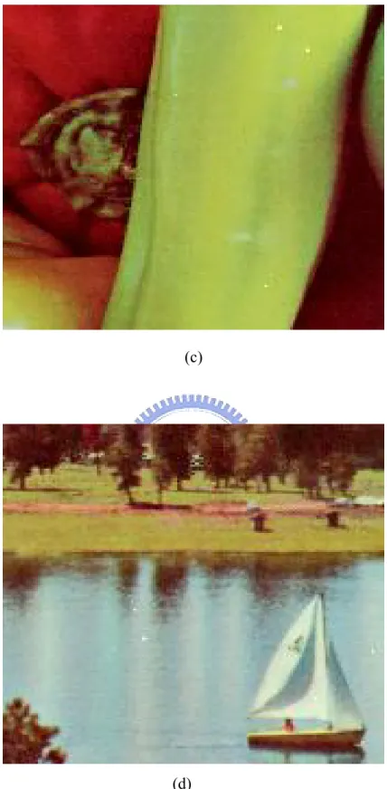
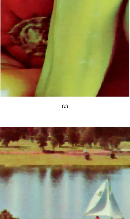
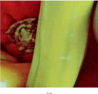
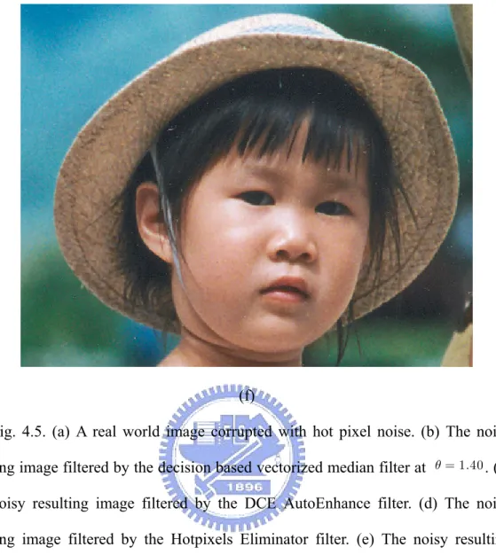
Fig. 4.5. (a) A real world image corrupted with hot pixel noise.

(b)The noisy resulting image filtered by the decision based vectorized median filter at ò= 1.40_.

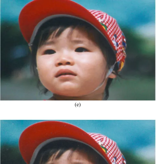
(c) The noisy resulting image filtered by the DCE AutoEnhance filter. (d) The noisy resulting image filtered by the Hotpixels Eliminator filter. (e) The noisy resulting image filtered by the vector directional filter. (f) The noisy resulting image filtered by the decision-based VDF.

32 Fig. 4.6. (a) A real world image corrupted with hot pixel noise.

(b)The noisy resulting image filtered by the decision based vectorized median filter with CMF at ò= 1.40_.

(c) The noisy resulting image filtered by the DCE AutoEnhance filter. (d) The noisy resulting image filtered by the Hotpixels Eliminator filter. (e) The noisy resulting image filtered by the vector directional filter. (f) The noisy resulting image filtered by the decision-based VDF.

35 Fig. 4.7. Definition of the chromaticity error for two vectors fˆ. 38

(10)

List of Tables

Table Ⅰ NMSE for the images. 39

Table Ⅱ MCRE for the images. 39

Table Ⅲ Noise detection and filtering of the image “AIRPLANE.” 40

Table Ⅳ Detection rate of the image “AIRPLANE.” 40

Table Ⅴ Noise detection and filtering of the image “LENA.” 41

Table Ⅵ Detection rate of the image “LENA.” 41

Table Ⅶ Noise detection and filtering of the image “PEPPERS.” 42

Table Ⅷ Detection rate of the image “PEPPERS.” 42

Table Ⅸ Noise detection and filtering of the image “SAILBOAT.” 43

Table Ⅹ Detection rate of the image “SAILBOAT.” 43

Table ⅩⅠ WPSNR comparisons of “Airplane,” “Lena,” “Peppers,” and “Sailboat” by five different filters with different ò3. 44

(11)

Chapter 1 Introduction

The digital cameras have almost become the necessities for every family around the world recently. People record their lives, traveling spots, celebrations, what ever the scenes they want to preserve, even trivial little things, they just need to press the shutter and keep the images in the memory or hardware storage for reviewing latter. However, the most popular types of the digital cameras are cheaper and less quality due to their simple designing and weak sensitivity of sensor. On account of reason mentioned just previously, these point and shoot cameras seem to be easy to incur noise and degrade images that users are not supposed to want it happens.

In this thesis, we are interesting in the image hot spot noise (also called hot spot like noise) reduction which is one topic of major researches for digital camera’s noise removing. The degraded pixels are commonly also named Hot Pixels [1], [2]. They will be explicitly expounded in latter chapters. The particular issue we will address is to construct a decision-based model to a suitable retrieval filter for post image process under the structure of digital camera system that may incur hot spot noise in capturing a picture.

1.1 Literature Survey

The noise reduction of image process has been investigated for decades. The origination of it was starting with monochrome image. Since the techniques of the digital camera hardware make progress at a tremendous pace, color images have

(12)

become the trend nowadays. However, those traditional methods, such as mean filter [3], conventional median filter (CMF) [4]–[7], vector median filter (VMF) [8], [9], and decision-based vectorized median filter (DBVMF) [10], are typically suitable for monochrome image process, as a result of exploiting only the intensity-information of processing image and especially are useful for impulsive or Gaussian noise removal. Though, these filters have not bad performances in the single channel image process and can be applying on multi-channel image process by combining with the concept of color space. Nevertheless, they are not color-originated concepts and beyond question must lose certain advantages because of making least use of the information in other two color spaces.

The general vector directional filter (GVDF) [11]-[13] is thus developed exuberantly in recent decades. This new approach is better getting close to the nut of concept rising in color space. GVDF separates the processing of vector-valued signals into directional processing and magnitude processing. Its instinctive color property from the view of color space leads to outstanding performance on multi-channel image process. GVDF applies not only in color image processing, but also in satellite image data processing and multi-spectral biomedical image processing. In this thesis, GVDF is modeled by a decision-based structure and is aiming at reducing hot spot noise, a defect observed in the digital camera system.

(13)

Chapter 2 Origination of Hot Spot Noise

2.1 Hot Spot Like Noise and Its Origination

“Hot pixel” is a general term used to describe bright or colored specks in an image. It stands for the overcharged、 misfires or destroying detail in the image. Various factors lead to yield this outcome. In general, some pixels in the sensor array of a digital camera are over sensitive to light of varying degrees as these pixels on the CCD have some abnormal charge leakage. Supposing long exposure or high temperature of the camera, the hot pixels appearing rate are increasing consequently and mostly they appear more frequently in images that were captured in low light condition. If hot spot noise is bad enough, it would be annoying on regular shots. That is why people pay so much attention to modify the post image process in the digital camera system.

A real size crop of a hot (Pink!) pixel on Nikon 990 at 1/11 second against a normal light background (a door) is shownin Fig. 2.1 [2].

Fig. 2.1. A real size crop of a hot (Pink!) pixel.

(14)

2.2 Template Noise

Since in the real world, we can only acquire the contaminated image that corrupted by hot spot like noise, it is impossible for us to figure out the performance of our designing from comparing original clean image and the processed image. To solve this problem, we construct a model to generate image noise that resembles the hot spot like noise and the algorithm is produced by observing the hot spot like noise in the corrupted images as the following steps [10].

1) First we inspect the hot pixel typical pattern model contained in a real world image, the blob nearly contains 3 â 2 pixels and hence a 3 â 2 noise mask has been chosen to be the hot pixel blob in an image.

2) Then we choose a window size of 3 â 3 blocks, each contains a sub-block blob of size 3 â 2 pixels. Let the blob containing the hot pixel to be in the center block of the window, there are 54 pixels in the extended window.

3) Using the column vector of 3 â 2 hot pixel blob as the center of an extended window of size 9 â 6 pixels, calculate the average u of this extended window by

u =Px(iàs,jàt)_N ììì(s,t) ∈ pixel in the extended window (1) where W is a window of size 9 â 6 pixels. Therefore, the noise pixels blob is n(i, j) = x(i, j) à u(i, j)|(i, j) ∈ pixels in the hot pixel blob, and there are six pixels in the hot pixel blob.

4) After having the simplest noise model, we add the noise blob into the original picture. Noise n(i, j) is add to an original image f(i, j) [14] to generate an image f1(i, j) corrupted by hot pixel noise by

(15)

f1(i, j) = f(i, j) + n(i, j) (2)

5) From the steps above, the noisy images were originated from the original images. Although we have already added the above noise in the template image, the contaminated image is still a little different from the ideal noise model. The noise pixel n(i, j) is needed to be adjusted for producing more closely replica of the true hot pixel noise. We observe that the hot pixel noise is somewhat proportional to the gray level of the local value of the pixel. To reflect this, we add the inversely factors pu(i, j) and the random number ra(i, j) to the noise pixel n(i, j). The nh(i, j) modified from n(i, j) is described below.

nh(i, j) = ô

1 +q_u(i,j)1 õ

n(i, j) 1 + ra(i, j)[ _{] (3)}

where ra(i, j) is a random number from 0 to 0.5 to allow some randomness. As mentioned above, the u(i,j)

1 q

in Eq. (3) is introduced to reflect the hot pixel is more eminent in the dark area than usual. By this setting, if u(i, j) is small, then u(i,j)

1 q

becomes large, and vice versa. Then n(i, j) as given by Eq. (2) is replaced by nh(i, j) on Eq. (3), and therefore,

fh(i, j) = f(i, j) + nh(i, j) (4)

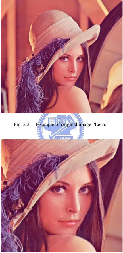
Following the steps, the hot pixel template noise can be easily added to a known image. Thus, we can have both the noisy and original images to assess the noise reduction performance in term of the quantification measures. An original image and its hot pixel noisy images are shown in Fig. 2.2 and Fig. 2.3. Fig. 2.2 is the original

(16)

image “Lena.” Fig. 2.3 is the noisy image with six mixed hot pixel noise patterns.

Fig. 2.2. Example of original image “Lena.”

(17)

Chapter 3 Decision-Based General Vector Directional

Filter for Hot Pixel Removal

The conventional filters for the image processing are mostly directly applying in the spatial domain by operating a specific or a set of functions individually on the independent channel of the given image. For the single channel image processing, different spatial filter has different effect respectively, but they are not good enough for the multi-channel image processing [11]. Separately processing on each channel and then reconstruct the multi-channel image seems to be less of consistency and fail to utilize the inherent correlation that is usually presented in multi-channel images. The general vector directional filter (GVDF) [11]-[13] provides a better approach than the spatial filters, those with inherent drawback, and considers the multi-channel image as a pack of vectors so as to take directional processing and magnitude processing into account. With this separation, GVDF can achieve good filtering on the color image, multi-channel image, for various noise source models.

3.1 General Vector Directional Filter

GVDF processes the input image in the concept of vector. A vector is formed in the color space [11], [15], and [16] by three-color components of an input pixel of the processing image, thus vector direction and magnitude are generated. GVDF can be divided into two components, the first component is the directional processing and the other is magnitude processing. In the first component of GVDF filter, the distance criterion is adopted by the angle difference and the stage aim in this step is to eliminate the atypical directions in the operating vectors. In this thesis, the introduced

(18)

directional processing is applying by a general vector directional filter, and its definition is as below [11].

Definition: The output of the generalized vector directional filter (GVDF), for input fi, i = 1, 2, ..., n

{ }, is the set SGD = GVDF f1, f2, ..., fn[ ], where SGD= fè (1)_{, f}(2)_{, . . ., f}(k)é_{, f}(i)

∈ f{ j, j = 1, 2, . . ., n} ∀i = 1, 2, ..., k.

Let

ëi

correspond to

fi

and be defined as

ë i= P j=1 n

A ( f i, f j) , i = 1, 2, ..., n.

where A(fi, fj) denotes the angle between the vectors fi and fj, 06 A(fi, fj)6 ù.

An ordering of the ëis

ë(1)6 ë(2)6 ... 6 ë(k)6 ... 6 ë(n). implies the same ordering to the corresponding fi_s

f(1)6 f(2)6 ... 6 f(k)6 ... 6 f(n)_.

The first

_k

terms of the ordered sequence f(i)_{constitute the output of the GVDF.}

GVDF outputs set of vectors whose angle difference from others in one processing are smaller. It trims out the unwanted or the more contaminated-likely pixel that particularly has atypical vector direction to the most of the other vectors. In other words, the output set of GVDF in the mask filtering can preserve the chromatic and intensity tendency in the local processing region since chromaticity and intensity for a color vector are highly correlated to the vector’s direction and its magnitude in the color cube. Indeed, chromatic difference between two color vectors is affected by the angle and the magnitude difference of the corresponding two color vectors.

(19)

Furthermore magnitude difference causes the intensity disparity. Thus, in this component, we want to ensure the output pixel’s chromaticity is not going too far away from its neighborhood.

In the second component of GVDF filter, the output of magnitude processing is obtained from specific gray-scale filter such as: the ë–trimmed mean [16], [17], the morphological open-close [18], and the multistage max/median [19]. Here the gray-scale median filter [16], [20] is introduced on the processing image. From this filter, we can appropriately substitute the possible outlier pixel with one that has more centered intensity in the output of component one , and that prevent from miss employing the substitute by selecting the pixel with more extreme intensity.

3.2 Decision-based Vector Directional Filter

Generally speaking, GVDF has good performance on the multi-channel image processing. When it is applied on the purpose of removing hot spot noise in the image processing, however, the output performance is barely satisfied. Moreover, it possibly changes too much details to retrieve the corrupted image. That is to say GVDF fails to preserve the most pixels in the original input image and it violates the original intention of our filter design. Consequently, we develop a decision-based vector directional filter (DBVDF) to enhance the performance of the GVDF.

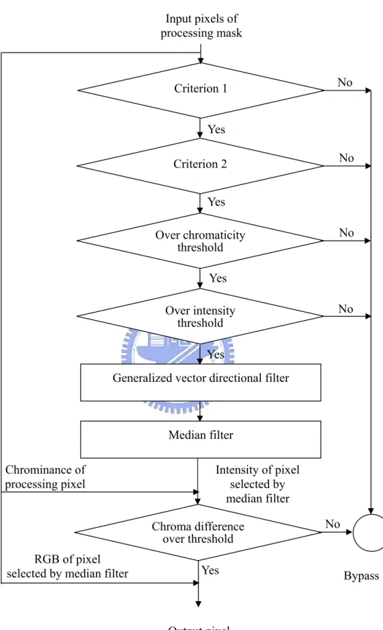
The algorithm of DBVDF involves 2 criterions and 5 stages. Two criterions for hot spot noise detection comes from the concept of using information of four neighborhood adjoin pixels, as shown in Fig. 3.1., to determine whether the processing pixel is to filter or not. Decisions made in these two criterions are

(20)

responsible for fast processing and high detection rate of proposed filter. The parameters in these two criterions are obtained from observing and summarizing. Besides, three of five stages have thresholds as decision. The 3rd stage is applied GVDF only, though the trimming length in the directional processing of GVDF is also a selected decision too. The whole DBVDF procedure is simply represented in the flowchart, as shown in Fig. 3.2. Thereafter, we will interpret the contents stage by stage explicitly.

Two Criterions:

Our proposed algorithm exploits low computation characteristic of two criterion to achieve the fast filtering and high noise detection rate. The definitions of Matrix

Cross, Matrix Cros12, Matrix Cross23 , Matrix Cross1234 and ò0, all in the intensity

sense, help to clearly describe the algorithm of adopted criterion in the first two components of DBVDF. It is noticed that the principal content in the criterion 1 is aiming at fast hot spot noise detection. The parameters in the description are experienced and experimental results. In addition, it is unnecessary to adjust these parameters for different processing images since the performances change slightly. In the criterion 2, there are four situations to comment. Different numbers of contaminated-likely neighborhood needs to be considered respectively. Indeed, the criterion 1 owns more severe restriction than criterion.

(21)

Definition:

Matrix Cross=sort{x(i,j-1),x(i-1,j),x(i,j+1),x(i+1,j)}. Matrix Cross12=Mean{Cross(1), Cross(2)}.

Matrix Cross23=Mean{Cross(2), Cross(3)}.

Matrix Cross1234=Mean{Cross(1), Cross(2), Cross(3), Cross(4)}.

ò0=(255-Cross1234)/(255-x(i,j)). Criterion 1: a) x(i,j)>=1.25âCross23 b) ò0>=1.45 c) x(i,j)=255 Criterion 2: a) x(i,j)>=235

b) x(i,j)>=1.2_âCross12 AND Cross(3)>=220 AND Cross(4)>=220 c) Cross(2)>=210 AND Cross(3)>=210 AND Cross(4)>=210 d) ò0>=1.35 AND Not{Cross(1)>=210 AND Cross(2)>=210 AND

Cross(3)>=210 AND Cross(4)>=210}

Stage 1:

In the region of our 3 â 3 moving processing mask, the intensity of every pixel is not supposed to vary too much because of the characteristic of nature light [1]. That is to say that intensities in limited-area local region seem to be somewhat continuous. Thus, we use the sum of intensity difference as a criterion to restrict the filtering so that the processing area with little intensity variation will be bypassed. It’s not only decreasing our image processing time but preserving the most uncontaminated part of the original input. Consequently, the output resembles the image without noise much more and the rate of correction gains high.

The threshold picked in this stage arises from the contents in the previous listed reasons. Considering a 3 â 3 moving processing mask as in Fig. 3.3, decision

(22)

Over chromaticity threshold Criterion 2 Criterion 1 Over intensity threshold Chroma difference over threshold

Generalized vector directional filter

Median filter Input pixels of processing mask Intensity of pixel selected by median filter Chrominance of processing pixel RGB of pixel selected by median filter

Output pixel

Fig. 3.2. Flow chart of decision-based vector directional filter.

Bypass No No No No No Yes Yes Yes Yes Yes

(23)

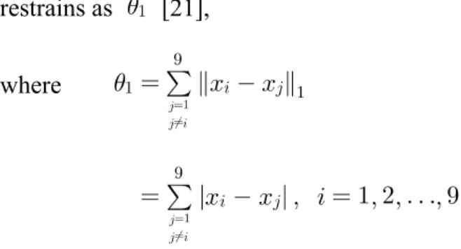
restrains as ò1_[21], where ò1=P j6=i j=1 9 xià xj k k1 =P j6=i j=1 9 xià xj | | , i = 1, 2, . . ., 9

xi_{and x}j denote the intensity of the indexed pixel if ò1_{is greater than the threshold picked in this stag, then the proposed decision} mechanism is meant to regard the processing pixel as an outlier one.

Stage 2:

As the assumption in the stage 1, the color difference in the neighborhood of

moving processing mask is supposed not to alter abruptly. In these two stages, we are expected to process comparatively normal contaminated-images with no abnormal intensity and color difference bounces. Once we filter a particular input that has a lot of edges in its detail, however, so long as the threshold selected in this stage be enlarged enough to prevent from modifying the complex color variation regions (usually refer to edges) as far as possible. Since contaminated pixels mostly are discontinuous in color with its neighbor clean pixels and usually have a great jump in every dimension of 3 color components with uncontaminated neighborhood, this stage employs the characteristic of the hot pixel noise to decide whether the moving mask is

x

1

x

2

x

3

x

4

x

5

x

6

x

7

x

8

x

9

(24)

going to be processing or just neglect the filtering in this pixel. This step saves lots of processing time again and even preserves the originality of the most pixels of input image further.

Considering a

_{3 â3 moving processing mask as in Fig. 3.2, decision restrain}

is selected by ò2, where ò2=P j6=i j=1 9 yià yj k k1 =P j6=i j=1 9 yià yj | | , j = 1, 2, . . ., 9

yi and yj_{denote the three principal chroma of the indexed pixel} if ò2_{is greater than the threshold picked in this stage, then the proposed decision} mechanism is meant to regard the processing pixel as an outlier one.

Both of the stage 1 and stage 2 are highly related to the performing time cost. It is because that they determine whether the processing pixel is to be filtering or not. By these two stage’s criterions, we can save the a large quantity of processing time cause proceeds on filtering the uncontaminated-likely pixels with the GVDF in the next stage would takes a huge amount of time for its vast complexity of

computations.

Stage 3:

Every pixel in the image can be seen as a vector as in Fig. 3.4. On account of color characteristic, we introduce the GVDF as a main filter in whole. The GVDF utilizes its principal viewpoint based on the color space concept and this is more close to the fundamental property in color image processing than any other filters. Although

(25)

GVDF costs considerably long time, it still has an outstanding performance in the multi-channels signal process. That’s the reason why we use the GVDF as a main filter [11] in the entire process. What is more in our design, the filter is appended the restrictions previously in this stage like those in stage 1 and stage 2, thus we can decrease the processing time effectively by the way of adequately choosing the more possible contaminated-likely pixels to handle.

The strategy here is to adopt the

_{3 â3}

moving mask too while signal length criterion should be take into consideration so that the output signal length of GVDF is not varying far from the adjoining pixels of input. In the algorithm of GVDF, we take half numbers of input signals (that is in general) to be the trimming target. Therefore, four input pixels that deviate from the other five inputs are passed over because they are seemed to be noise-like ones.

Stage 4:

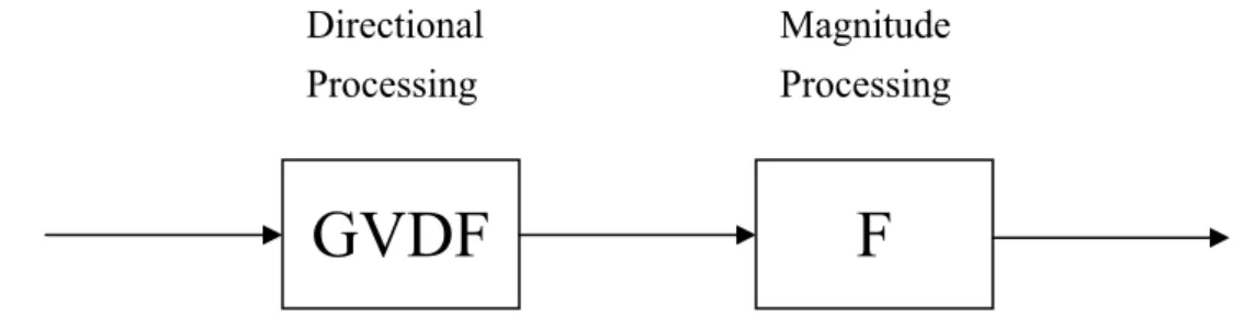
In fact, the GVDF uses a cascade of directional processing and magnitude processing that is shown in Fig. 3.5. As we describe at the previous chapter, three

(26)

Fig. 3.4. Perspective representation of the color cube.

filters have been used for the step of magnitude processing: the ë-trimmed mean [16], [17] the morphological open-close [18], and the multistage max/median [19].

However we do not expect to replace the processing pixel directly with the output of vector directional filter (VDF) [11] or output of GVDF cascaded with one of these three different kinds of filters. Instead of those filters, the mean filter in the intensity sense is adopted in the step of magnitude processing. Nevertheless it is just only a reference so that we can make decision of what pixel is selected to replace the current processing contaminated-likely pixel. In other words, decision in this stage is that we substitute the contaminated-like pixel (judged via our algorithm) by the one whose intensity is more probably closed to the original uncontaminated pixel, of course, they are all in the moving mask. It really makes the retrieval pixel with intensity more continuous nearby the processing region.

The substitution is implemented in all the three color channels, thus, the output turns to be more excellent and more continuous with neighborhood in the color sense than that directly processed by GVDF and cascaded ordinary filter.

Stage 5:

In order to restore the most uncontaminated pixel of the input image, the last criterion is to let the output of our design much more resemble the original without too much artificial alteration. It is compensating for the condition once our decision goes wrong that results in filtering the clean pixel. We set a threshold ò3 to achieve

(27)

this goal in this stage. First we duplicate a copy of original input image. If the chromatic difference (absolute value) of the processing pixel in the original contaminated image and the output of stage 4 is smaller than ò3, then we do not modify the local processing pixel in the copy image. In case of the difference is greater than the threshold, we substitute the processing pixel in the duplicated image by the output of stage 4. In other words, we try to preserve the most original appearance in the input image again. The threshold should not be set too low so that the image contains too much artificial modification and most of that often are somehow dissimilar from the original. On the other hand, the duplicated copy may be remain unchanged for the most part as input image if the threshold is set too high so that we lose to filter out the hot spot like noise.

To summarize our design, we develop a decision-based GVDF applying on multi-channel image processing for removing the hot pixel like noise. The GVDF with a proper decision criterion is good because it would considerably reduce the required time for processing and attain a more excellent performance than that is implemented by GVDF only. Consequently we design a five-stage decision-based GVDF that considers both the chromaticity and the intensity content. In the simulation section, we will discuss its advantage by some assessment criterion.

Fig. 3.5. Multi-channel image processing using a cascade of directional processing and magnitude processing.

GVDF

F

Directional Processing

Magnitude Processing

(28)

Chapter 4 Simulation Results

We will show the efficiency of the DBVDF comparing against the GVMF with respect to the processing time. Moreover, quantitative measures in terms of the performance of each filter have also been provided. Of course, the experimental results in images will be shown as well.

4.1 Image with Synthetic Hot Pixel Noise

4.1.1 Experimental Results of the Decision-Based

Vectorized Median Filtering

The best threshold of the decision-based Vectorized Median Filter (DBVMF) has been found around 1.40. The experimental results for the commonly adopted images “Airplane,＂ “Lena,＂ “Peppers,＂ “Sailboat,＂ with the threshold ò=1.40 from the thesis [10] published in 2003 are shown in Fig. 4.1. We show the zoomed images so that the details could be revealed. Obviously, it can be seen that some hot spot noise remains in the filtered image and the sharpness of the image is lost over the whole image. That is, the DBVMF fails to filter all the hot spot noise in the corrupted image and diverts the attention of the viewer from the subject of the filtered image.

(29)

(a)

(30)

(c)

(d)

Fig. 4.1. (a) Zoomed “Airplane＂ filtered by the decision-based VMF with

ò= 1.40_{. (b) Zoomed “Lena＂ filtered by the decision-based VMF with} ò= 1.40_{. (c)}

Zoomed “Peppers＂ filtered by the decision-based VMF with ò= 1.40 _{. (d)}

(31)

4.1.2 DCE AutoEnhance and Hot Pixels Eliminator

DCE AutoEnhance and Hot Pixels Eliminator [22], [23] which are famous web sites concerning hot pixel reduction in the world wide web. The algorithms of these two methods are not available but executable programs are provided in the web. It has been proved that the decision-based VMF outperforms both of these two methods. Fig. 4.2 shows the filtered Airplane, Lena, Peppers, and Sailboat images from DCE AutoEnhance and Hot Pixels Eliminator, respectively. Again, we show the zoomed images for the purpose of clearly observing the texture and color contents in the filtered images. If we compare the images filtered by these two methods with the input processing images, we can find that the color and luster alter too much in the filtered images that we might think they possibly are not the results of the processing image. The filtered images looks like being shot under different light sources or in which the contents are appeared to be in different hues and saturations. Despite the two methods filtering out nearly all the hot spot noise, they are barely satisfied for the severe drawback of losing nature color of original input processing images.

Although DBVMF, DCE AutoEnhance, and Hot Pixels Eliminator have their defect respectively, they all possess the characteristic of low processing time which is the ultimate drawback of the VDF and DBVDF.

(32)

(a)

(33)

(c)

(d)

Fig. 4.2. (a) Zoomed “Airplane＂ filtered by the DCE AutoEnhance filter. (b) Zoomed “Airplane＂ filtered by the HotPixels Eliminator filter. (c) Zoomed“Lena＂ filtered by the DCE AutoEnhance filter. (d) Zoomed “Lena＂ filtered by the HotPixels Eliminator filter.

(34)

4.1.3 Generalized Vector Directional Filter and

Decision-Based Vector Directional Filter

Fig. 4.3 and Fig. 4.4 show the experimental results via GVDF and DBVDF respectively. We may see that images filtered by DBVDF has effectively reduced the hot spot noise, and better preserve the texture of the original image than GVDF. The output images of DBVDF are more realistic because of the fundamental characteristic of the DBVDF algorithm. And it might be easily perceived since images filtered by DBVDF are more natural in coloring comparing to those filtered by GVDF. Although the proposed filter outperforms GVDF, the slightly excessive pixels filtered by DBVDF seem to be observable than the other type of filters, because of over detection mentioned previously. However, our proposed filter bypasses the most uncontaminated pixels to preserving the details and sharpness of the input processing images. The quantitative tables will be listed in the following section and we will show the excellence of DBVDF comparing to the other filters introduced in this thesis, especially comparing to GVDF which is the basic model adopted in our filter＇s framework.kkkkkkkkkkkkkkkkkkkkkkkkkkkkkkkkkkkkkkkkkkkkkkkkkkframework

(35)

(a)

(36)

(c)

(d)

Fig. 4.3. (a) Zoomed “Airplane＂ filtered by the generalized vector directional filter. (b) Zoomed “Lena＂ filtered by the generalized vector directional filter. (c) Zoomed “Peppers＂ filtered by the generalized vector directional filter. (d) Zoomed “Sailboat＂ filtered by the generalized vector directional filter.

(37)

(a)

(38)

(c)

(d)

Fig. 4.4. (a) Zoomed “Airplane＂ filtered by the decision-based vector directional filter. (b) Zoomed “Lena＂ filtered by the decision-based vector directional filter. (c) Zoomed “Peppers＂ filtered by the decision-based vector directional filter. (d) Zoomed “Sailboat＂ filtered by the decision-based vector directional filter.

(39)

4.1.4 Experiment of Real World Image Corrupted with

Hot Pixel Noise

Here, two images corrupted with the real hot pixel noise will be tested. Figs. 4.5 and 4.6 show the tested image and filtered image, respectively.

(a)

(40)

(b)

(c)

(41)

(d)

(42)

(f)

Fig. 4.5. (a) A real world image corrupted with hot pixel noise. (b) The noisy resulting image filtered by the decision based vectorized median filter at ò= 1.40_{. (c)}

The noisy resulting image filtered by the DCE AutoEnhance filter. (d) The noisy resulting image filtered by the Hotpixels Eliminator filter. (e) The noisy resulting image filtered by the vector directional filter. (f) The noisy resulting image filtered by the decision-based vector directional filter.

(43)

(a)

(44)

(c)

(d)

(45)

(e)

(f)

Fig. 4.6. (a) A real world image corrupted with hot pixel noise. (b) The noisy resulting image filtered by the decision based vectorized median filter with CMF at

ò= 1.40. (c) The noisy resulting image filtered by the DCE AutoEnhance filter. (d)

The noisy resulting image filtered by the Hotpixels Eliminator filter. (e) The noisy resulting image filtered by the vector directional filter. (f) The noisy resulting image filtered by the decision-based vector directional filter.

(46)

4.2 Performance Comparison

4.2.1 Normalized Mean Square Error and Mean

Chromaticity Error

From the experimental results above, the resulting images by the introduced filter: BDVMF, DCE AutoEnhance, VDF, and DBVDF methods are difficult to assess visually. We find that the proposed DBVDF method provides high efficiency in eliminating the hot spot noise by the human vision perception. Two quantitative measures are employed to compare the performance of these filters [11]. The first is the normalized mean squared error NMSE( _{), which is a standard measure as given} by NMSE = _P i=0 N1 P j=0 N2 f(i,j) k k2 P i=0 N1 P j=0 N2 f_{(i,j)àfê(i,j)} k k2 , (5)

where N1 and N2 are the image dimensions, and f(i, j) and fê(i, j) denote the original and the estimated image vector at pixel (i, j), respectively. The second measure is the mean chromaticity error MCRE( _{). Since the GVDF and DBVDF} operate as chromaticity filters, consequently their performance in terms of chromaticity error should be evaluated. MCRE is defined as

MCRE = N1N2 P i=0 N1 P j=0 N2 C f(i,j),fê(i,j)[ ] , (6)

where N1,N2,f(i, j), and fê(i, j) are as in (5) and C f(i, j), fê(i, j)

h i

is the chromaticity error between vectors f(i, j), and fê(i, j). It is defined as the distance

(47)

P Pê between the two points P and Pê, which are the intersection points of f(i, j), and fê(i, j) with the Maxwell triangle, respectively. This is shown graphically in Fig. 4.7 and we summarize the results in Tables I and II which respectively show the NMSE and MCRE of the various filters we introduced. However, we cannot, in practice, calculate the NMSE or MCRE to compare the efficiency about the real world corrupted images with our proposed DBVDF and the other filters owing to the lack of the images uncorrupted with the hot pixel noise.

4.2.2 Noise Detection and Weighted Peak Signal to

Noise Ratio

The noise detection and filtering rate of hot spot noise for the images “Airplane,” “Lena,” “Peppers,” and “Sailboat” are shown in Tables VI-X. It is to be noticed that the true positive values of our proposed filter are almost 100% for these four images and false negative values are higher than the other filters. That is, our proposed filter detects all the hot spot noise in the contaminated images and keeps most uncorrupted pixels unchanged. In addition to the quantitative evaluation presented above, a qualitative evaluation is necessary since the visual assessment of the processed image is, the must subjective measure of the efficiency of any method. Therefore we introduce weighted peak signal to noise ratio WPSNR( _{) to stress on} reducing the hot spot noise or not of the filters. The weight vector W~ = W( 1, W2, W3) is

adopted to reflect the hot pixels by weights to account the removing capability of the filters. In the above, W1 indicates the weight to emphasize the hot spot noisy pixel

(48)

indicates the weight to the hot spot noisy pixel not detected to be contaminated. W3

indicates the weight to the clean pixel is detected contaminated and filtered. The processing results of the introduced filters are shown in Tables III–XI.

It is obviously seen that our proposed filter is better than the other filters in the three of four processing images on the access measure of NMSE and MCRE, even in WPSNR. We might find that when the threshold ò3 increases in the experiment, the false detection of hot spot noise of our proposed filter decreases meanwhile leaves more uncontaminated pixels bypass. However, there are more hot spot noise not detected in the mean time, that represents the capability of filtering out hot spot noise decreases. The adjustability is the crucial reason that makes our filter more competitive and selective than DBVMF.

Green Blue Red Maxwell Triangle fˆ f Pˆ P

0

(49)

TABLE I

NMSE (×₁₀à6) FOR THE IMAGES

filters or ò3 Airplane Lena Peppers Sailboat

DBVMF 104.4 142.4 279.2 500.8 DBVMF+CMF 104.3 139.9 262.9 487.0 DCE 15240.4 19484.8 10026.3 9207.6 GVDF 5086.0 5159.5 9347.8 14460.9 DBVDF 100 113.0 193.3 260.0 550.8 110 112.5 191.5 258.4 542.6 120 110.7 186.3 255.8 532.1 130 108.2 180.6 252.4 516.1 140 107.3 174.7 246.5 500.2 150 104.9 168.1 234.2 484.7 160 102.1 160.2 223.2 464.3 170 98.2 157.2 217.4 440.8 180 91.1 152.1 209.7 410.6 190 88.9 147.6 208.8 382.4 200 87.4* 132.6* 193.7* 361.4* GVDF: cascaded with median filter

Thresholds in stage 1 and 2: both defined as 500

TABLE II

MCRE (×₁₀à6) FOR THE IMAGES

filters or _ò3 Airplane Lena Peppers Sailboat

DBVMF 17.3 22.0 26.0 18.4* DBVMF+CMF 17.3 22.0 25.4 18.4* DCE 361.1 1725.1 588.1 885.4 GVDF 1570.2 1051.8 2645.7 4107.2 DBVDF 100 11.3 21.3 24.9 57.8 110 11.1 21.0 24.3 56.9 120 10.9 20.2 23.8 55.0 130 10.7 19.3 23.4 53.2 140 10.5 18.3 22.5 50.7 150 10.3 17.7 20.0 48.8 160 10.1 16.7 18.9 46.2 170 9.6 16.5 17.5 43.2 180 9.3 16.0 16.7 38.7 190 8.8 15.2 16.3 35.8 200 8.5* 13.3* 14.5* 33.2

GVDF: cascaded with median filter

(50)

TABLE III

NOISE DETECTION AND FILTERINGOFTHEIMAGE “AIRPLANE” (PIXELS)

filters or ò3 True Positive True Negative False Positive False Negative

DBVMF 49 100 204943 57052 DBVMF+CMF 49 100 204942 57053 DCE 133 16 261994 1 GVDF 149 0 229241 32754 DBVDF 100 142 7 203 261792 110 137 12 194 261801 120 133 16 180 261815 130 129 20 161 261834 140 115 34 147 261848 150 108 41 132 261863 160 99 50 117 261878 170 87 62 96 261899 180 83 66 75 261920 190 73 76 62 261933 200 64 85 52 261943

Total numbers of pixel: 512â512 GVDF: cascaded with median filter

TABLE IV

DETECTION RATEOF THEIMAGE “AIRPLANE” (%)

True False

filters or _ò3 Positive Negative Positive

(51)

TABLE V

NOISE DETECTION AND FILTERINGOFTHEIMAGE “LENA” (PIXELS)

filters or _ò3 True Positive True Negative False Positive False Negative

TABLE VI

DETECTION RATEOF THEIMAGE “LENA” (%)

True False

(52)

TABLE VII

NOISE DETECTION AND FILTERINGOFTHEIMAGE “PEPPERS” (PIXELS)

TABLE VIII

DETECTION RATEOF THEIMAGE “PEPPERS” (%)

True False

(53)

TABLE IX

NOISE DETECTION AND FILTERINGOFTHEIMAGE “SAILBOAT” (PIXELS)

TABLE X

DETECTION RATEOF THEIMAGE “SAILBOAT” (%)

True False

filters or ò3 Positive Negative Positive

DBVMF 66 34 66 34 DBVMF+CMF 66 34 66 34 DCE 100 0 100 0 GVDF ₁₀₀₀₈₈₁₂ DBVDF 100 90 10 0 100 110 89 11 0 100 120 87 13 0 100 130 87 13 0 100 140 87 13 0 100 150 84 16 0 100 160 82 18 0 100 170 80 20 0 100 180 78 22 0 100 190 76 24 0 100 200 73 27 0 100

(54)

TABLE XI

WPSNR comparisons of “Airplane,＂ “Lena,＂ “Peppers,＂ and “Sailboat＂ by five different filters with different ò3

(a)

filters or _ò3 Airplane Lena Peppers Sailboat

Thresholds in stage 1 and 2: both defined as 500 (b)

(w1, w2, w3)=(40,40,20) WPSNR DBVMF 23.66 25.04 23.01 20.05 DBVMF+CMF 23.67 25.12 23.23 20.18 DCE 3.06 4.44 8.00 7.71 GVDF 7.84 10.22 8.43 5.76 DBVDF 100 25.15 25.04 24.52 20.04 110 25.14 25.09 24.55 20.11 120 25.19 25.23 24.60 20.19 130 25.27 25.37 24.67 20.32 140 25.19 25.52 24.78 20.46 150 25.23 25.71 25.04 20.59 160 25.28 25.91 25.28 20.76 170 25.32 25.90 25.33 20.97 180 25.61* 25.93 25.49 21.26 190 25.54 25.92 25.41 21.55 200 25.44 26.23* 25.71* 21.75* (w1, w2, w3)=(50,50,20) WPSNR DBVMF 23.18 24.57 22.67 19.88 DBVMF+CMF 23.18 24.65 22.86 20.00 DCE 3.06 4.43 7.94 7.70 GVDF 7.83 10.22 8.43 5.76 DBVDF 100 25.00 24.87 24.33 19.93 110 24.98 24.91 24.36 19.98 120 25.01 25.04 24.41 20.06 130 25.07 25.17 24.48 20.19 140 24.94 25.31 24.59 20.33 150 24.94 25.49 24.83 20.45 160 24.94 25.66 25.06 20.60 170 24.91 25.59 25.07 20.79 180 25.15* 25.57 25.21 21.07 190 25.00 25.50 25.09 21.33 200 24.84 25.69* 25.33* 21.50*

(55)

(c)

4.2.3 Time Consumption

Table XII shows our proposed DBVDF saves lot of processing time via GVDF. In fact, the elapsed time is correlated to the threshold we defined in DBVDF and the complexity of the input image. Obviously, huge computational complexity significantly limits GVDF practical usability. It is proved that DBVDF considerably reduces the computational complexity of the GVDF because of its decision-based algorithm. The speed improvement achieved nearly 100 times of simply applying GVDF only. (w1, w2, w3)=(60,60,10) WPSNR DBVMF 23.78 25.25 23.81 21.84 DBVMF+CMF 23.78 25.31 23.92 21.96 DCE 6.04 7.38 10.56 10.66 GVDF 10.83 13.21 11.43 8.76 DBVDF 100 27.10* 26.81 26.22 22.19 110 27.00 26.84 26.25 22.23 120 26.94 26.95 26.29 22.27 130 26.87 27.00 26.34 22.38 140 26.49 27.07 26.42 22.49 150 26.32 27.21 26.60 22.57 160 26.14 27.24* 26.78* 22.64 170 25.81 26.93 26.58 22.74 180 25.83 26.65 26.64 22.90 190 25.43 26.31 26.34 23.03 200 25.06 26.10 26.36 23.06*

(56)

TABLE XII

PROCESSING TIME (sec) FOR EACH FILTER

Image Airplane Lena Peppers Sailboat

VDF 2859.45 2803.00 2796.64 2807.89

DBVDF 40.62 25.28 28.39 32.34

Thresholds in stage 1 and 2: both defined as 500 _ò₃: defined as 100

(57)

Chapter 5 Conclusion

In this thesis, a decision-based vector directional filter is proposed to reduce the hot spot noise in the images. In this scheme, we construct a two criterion and five-stage filter that saves lot of the processing time and preserves the image details better than the GVDF, as demonstrated in the experimental results. Indeed, we enhance the functionality of GVDF and exploit its original chrominance characteristic, which is very important in visual perception of color image, when applying on reducing the hot spot noise. Moreover, it can be implemented easily. Comparing to the conventional filter, DBVMF, and the famous filters on the web site: DCE AutoEnhance, DBVDF outperforms each of these filters. In the image processing, DBVDF demonstrates its effectiveness in less time consumption comparing to GVDF and in fidelity to the original uncontaminated image than the other filters. These features are reflected on the measures of NMSE and the detection rate. In the era of color image, DBVDF is supposed to be the most attractive filter for its internal color conception. Of course, DBVDF is on using in recovering the contaminated images corrupted by the hot spot noise.

Though DBVDF improves GVDF in both time consumption and details preservation, it is difficult to implement DBVDF in the real time designing mainly because it is still intrinsically computative. Future work about this field should be concentrated on the promotion of time efficiency, and that is expected to be a great challenge, a giant milestone in the meantime, in the progress of vector directional filter.

(58)

References

[1] “Effective Noise Reduction & Detail Optimization: An Analysis & Post

Capture Process Model,’’ nik multimedia, Inc,2003. [2] “Digital Camera Experiments,” [Online]. Available HTTP:

http://webpages.charter.net/bbiggers/DCExperiments/html/hot_pixels.html October 1, 2003.

[3] K. M. Singh and P. K. Bora, Adaptive Rank-ordered Mean Filter for Removal of

Impulse Noise from Images, Indian Institute of Technology, Guwahati-781039, India.

[4] J. S. Lim, Two-Dimensional Signal and Image Processing, Englewood Cliff,

N.J: Prentice-Hall, 1990.

[5] J. M. Tukey, “Nonlinear (nonsuperposable) methods for smoothing data,” in

Proc. Congr. EASCON, p. 673, 1974.

[6] T. Chen and H. R. Wu, “Adaptive Impulse Detection Using Center-Weighted

Median Filters,” IEEE Signal Processing Letters, vol. 8, No 1, pp. 1–3, Jan. 2001.

[7] S. J. Ko and Y. H. Lee, “Center Weighted Median Filters and Their Applications

to Image Enhancement,” IEEE Transactions on Circuits and System: Analog and Digital Signal Processing, vol. 38, No 9, pp. 984–993, Sept. 1991.

[8] J. Astola, P. Haavisto, and Y. Neuvo, “Vector Median Filters,” Proc. IEEE, vol.

78, no. 4, pp. 690–710, Apr. 1990.

[9] M. Barni, V. Cappellini, and A. Mecocci, “Fast Vector Median Filter Based on

Euclidean Norm Approximation,” IEEE Signal Processing Letters, vol. 1, No 6,

(59)

[10] C. M. Lee, “Decision-Based Vectorized Median Filter for Hot Pixel Noise

Removal,” thesis from the Department of Electronic and Control Engineering of the National Chiao Tung University in Taiwan, June. 2003.

[11] P. E. Trahanias and A. N. Venetsanopoulos “Vector Directional Filters-A New

Class of Multi-channel Image Processing Filters,” IEEE Transactions on Image Processing, vol2. 4, No 6, pp. 528–534, October. 1993.

[12] K.N. Plataniotis, D. Androutsos, and A. N. Venetsanopoulos, “Vector Directional Filters: An Overview,” Proceedings, Canadian Conference on Electrical and Computer Engineering, May 25–28, 1997, St. John's, NF,

Canada, pp. 106–110, 1997.

[13] K.N. Plataniotis, D. Androutsos, and A. N. Venetsanopoulos, “Color Image

Processing Using Adaptive Vector Directional Filters,” IEEE Transactions on Circuits and System-II: Analog and Digital Signal Processing,vol. 45, No 10,

pp. 1414–1419, October. 1998.

[14] A. J. Bardos and S. J. Sangwine, “Measuring noise in colour images,” in Proc. IEE Colloquium on Non-Linear Signal and Image Processing, no. 284, 22

May 1998.

[15] R. C. Gonzalez and R. E. Woods, Digital Image Processing, New York: Second Edition, 2001.

[16] I. Pitas and A. N. Venetsanopoulos, Nonlinear Digital Filters-Principles and Applications.Norwell, MA: Kluwer Academic Publ., 1990.

[17] J. Bee Bednar and Terry L. Watt, “Alpha-Trimmed Means and Their

Relationship to Median Filters,” IEEE Transactions on Acoustics, Speech, and Signal Process, vol. Assp–32, No 1, pp. 145–153, February. 1984.

[18] P. A. Maragos and R. W. Schafer, “Morphological filters-part I: their

(60)

Transactions on Acoustics, Speech, and Signal Process,’’ vol. 35, No 8, pp.

1155–1169, Aug. 1987.

[19] G.. R. Arce and R. E. Foster, “Detail-preserving ranked-order based filters for

image processing,” IEEE Transactions on Acoustics, Speech, and Signal Process, vol. 37, pp. 83–98, Jan. 1989.

[20] A. K. Jain, Fundamentals of Digital Image Processing, New Jersey:

Prentice-Hall, 1989.

[21] S. K. Pal and A. Rosenfeld, “Image enhancement and thresholding by

optimization of fuzzy compactness, ”IEEE Pattern Recognition Letters, vol. 7,

No 1, pp. 77–86, Feb. 1988.

[22] “DCE AutoEnhance Automatic Digital Camera Enhance and batch processor,”,

[Online]. Avaliable HTTP: http://www.mediachance.com/dce/index.html, 2000.

[23] “HotPixel Eliminator to fight against HotPixels,”, [Online]. Avaliable HTTP:

消除影像熱像素雜訊之選擇性向量指向濾波器

國 立 交 通 大 學

電 機 與 控 制 工 程 研 究 所

碩 士 論 文

消除影像熱像素雜訊

之選擇性向量指向濾波器

Decision-Based Vector Directional Filter

for Hot Pixel Noise Removal

研 究 生：陳 瑞 俊

指導教授：張 志 永 博 士

消除影像熱像素雜訊

之選擇性向量指向濾波器

Decision-Based Vector Directional Filter

for Hot Pixel Noise Removal

學 生: 陳 瑞 俊 Student: Jui-Chun Chen

指導教授: 張 志 永 Advisor: Jyh-Yeong Chang

國 立 交 通 大 學

電 機 與 控 制 工 程 學 系

碩 士 論 文

A Thesis

Submitted to Department of Electrical and Control Engineering

College of Electrical Engineering and Computer Science

National Chiao Tung University

in partial Fulfillment of the Requirements

for the Degree of Master in

Electrical and Control Engineering

June 2004

Hsinchu, Taiwan, Republic of China

中華民國 九十三 年 六 月

消除影像熱像素雜訊

之選擇性向量指向濾波器

學 生: 陳 瑞 俊 指 導 教 授: 張 志 永 博士

國立交通大學電機與控制工程所

摘 要

Decision-Based Vector Directional Filter

for Hot Pixel Noise Removal

Institute of Electrical and Control Engineering

ABSTRACT

CONTENTS

ABSTRACT (CHINESE) i

ABSTRACT (ENGLISH) ii

CONTENTS iv

LIST OF FIGURES vi

LIST OF TABLES viii

Chapter 1 Introduction 1

Chapter 2 Origination of Hot Spot Noise 3

Chapter 3

Decision-Based Generalized Vector Directional

Filter for Hot Pixel Removal 7

Chapter 4 Simulation Results 18

Chapter 5 Conclusion 47

REFERENCES 48

List of Figures

List of Tables

Chapter 1 Introduction

1.1 Literature Survey

Chapter 2 Origination of Hot Spot Noise

2.1 Hot Spot Like Noise and Its Origination

2.2 Template Noise

Chapter 3 Decision-Based General Vector Directional

Filter for Hot Pixel Removal

3.1 General Vector Directional Filter

Let

correspond to

and be defined as

k

3.2 Decision-based Vector Directional Filter

Two Criterions:

Stage 1:

Stage 2:

x

x

x

x

x

x

x

x

x

3 â3 moving processing mask as in Fig. 3.2, decision restrain

國立交通大學

電機與控制工程研究所

碩士論文

研究生：陳瑞俊

指導教授：張志永博士

學生: 陳瑞俊 Student: Jui-Chun Chen

指導教授: 張志永 Advisor: Jyh-Yeong Chang

國立交通大學

電機與控制工程學系

碩士論文

中華民國九十三年六月

學生: 陳瑞俊指導教授: 張志永博士

摘要

_k

_{3 â3 moving processing mask as in Fig. 3.2, decision restrain}

_{3 â3}