時空關聯之市區短期交通預測模式

行政院國家科學委員會專題研究計畫 成果報告

時空關聯之市區短期交通預測模式

研究成果報告(精簡版)

計 畫 類 別 ： 個別型 計 畫 編 號 ： NSC 99-2221-E-009-094- 執 行 期 間 ： 99 年 08 月 01 日至 100 年 07 月 31 日 執 行 單 位 ： 國立交通大學運輸科技與管理學系（所） 計 畫 主 持 人 ： 黃家耀 報 告 附 件 ： 出席國際會議研究心得報告及發表論文 處 理 方 式 ： 本計畫可公開查詢

中 華 民 國 100 年 10 月 30 日

1

時空關聯之市區短期交通預測模式

摘要 在市區的交通管理系統上，交通流量的時空關聯關係是十分重要。大量的文獻都以單變 量的時間序列為研究對象，並不考慮多變量之間的空間關係。本研究提出一空間聯關的 交通流量預測模型，以 STARIMA 模型為基礎，並根據量測點的相對位置建立路網設 定的方式。本研究以台北市一區域為範例分析對象，說明所提出的模型有效表達多個量 測點的時間與空間的相關性。

Short-term urban traffic forecasting with spatio-temporal correlations

ABSTRACT

The spatial-temporal evolution of traffic flow in an urban network is essential in developing effective traffic management systems for urban areas. Most of previous models of short-term traffic forecasting make use of time-series analysis, without the components to consider the spatial correlations between the measurement locations in the network. In this paper, we present a space-time modeling approach to the traffic flow forecasting problem. A space-time autoregressive integrated moving average (STARIMA) model is introduced to develop an efficient estimation and forecasting model, in which the spatial correlations of the time series are modeled with a network specification incorporating physical neighborhood structure. A case study using the traffic data in Taipei city, Taiwan, is performed, and the experimental results reveal that the proposed model is suitable for traffic flow forecasting in urban network with multiple locations which are correlated both spatially and temporally.

I. INTRODUCTION

With the development of technologies in telemetric, the interests and applications of Intelligent Transportation Systems (ITS) have been growing in recent years. The implementations in real-time such as dynamic traffic information provisions and dynamic traffic control require the forecasting of traffic conditions in near future. Majority of previous literature have focused on the modeling of observations from a single site using univariate approaches, and there are recent studies to investigate the relationships between sites with multivariate approaches [1]. To facilitate an effective traffic control system in an urban area, it would be more desirable to understand the evolution of traffic patterns in a transportation network over both space and time.

Modeling traffic flow in urban arterials is challenging. There are many origins and destinations with multiple route choices for travelers in the network, and there may be disturbances on the roads such as traffic signals and mixed traffic. Recent empirical investigations demonstrated the dependency of traffic data in the spatial and temporal domains [2], [3]. Therefore a forecasting model for urban area considering the spatial

2

relationships of traffic flow at different adjacent locations is appropriate and necessary. In this paper, an approach for the space-time modeling of traffic flow for urban roads is proposed. The univariate autoregressive integrated moving average (ARIMA) model, which has been implemented successfully in the traffic flow forecasting problem [4], [5], is extended. A space-time autoregressive integrated moving average (space-time ARIMA, or STARIMA) model is introduced in this paper to develop a multivariate yet computational efficient approach taking into account the physical space-time relationships for detector locations. Some practical considerations and specifications for urban traffic network are discussed.

II. METHODS FOR SHORT-TERM TRAFFIC FORECASTING

Forecast implies prediction of future events and conditions [6], and forecasting of traffic conditions in the near future is essential in the applications of traffic management and control in Intelligent Transportation Systems. A wide variety of short-term traffic forecasting problems have been investigated during past decades, and the scopes of them were diverse [7]. For the purpose of traffic management in urban arterials, models to understand the traffic for a wide area of the network are particularly necessary. The exploitation of multivariate time series techniques may provide better insight and interpretation of the hidden relationships. The modelling of spatial-temporal domain of traffic data has been receiving attention recently. Yue and Yeh [2] investigated the spatio-temporal dependency of traffic flow, and identified that the cross-correlation and time lags between stations would be different for different time period (e.g. morning period, evening period and off-peak) and traffic conditions. Cheng et al. [3] also obtained similar conclusions with an empirical investigation using London's road network data, and they concluded that spatio-temporal network autocorrelation structure should be dynamic and heterogeneous in both space and time.

III. THEORETICAL BACKGROUND

The space-time autoregressive integrated moving average (STARIMA) model is characterized with the autoregressive and moving average forms of multiple time series lagged in both space and time to incorporate the spatial correlations of the time series data [8]. It can be viewed as a special case of the vector ARMA (VARMA) model. VARMA is a multivariate version of ARMA, and supposes a general relationship of dependences between multiple time series [9]. It requires estimation of covariance matrix of the time series, and therefore the number of parameters to be estimated is a multiple of the square of the time series number. When the number of time series is large, it is generally difficult to calibrate a VARMA model in real applications.

STARIMA assumes a restricted form of the covariance matrix by specifying a spatial dependence structure of the time series measured over a space, and the number of coefficients in the model can be reduced. This is an appropriate assumption for the traffic measurements in

3

an urban road network, because traffic at a site is influenced by upstream and nearby traffic conditions.

A. Network specification

Assume that zi

( )

t ,i=1,2,...,N are N time series data which are stationary or made

stationary by differencing transformation, and z is the corresponding N

( )

t ×1 vector. Let L( )l

be the spatial lag operator of order l, defined as

( )

t z

( )

t z L(0) _i = _i (1) ( )

_{( )}

_∑

( )

_{( )}

= = N j j l ij i l t z w t z L 1 for l >0 (2)

in which w are a set of weightings capturing the spatial dependencies of how the time _ij(l) series data collected at location i is affected by location j at spatial order l. The spatial order accounts for the hierarchical structure, such that nearer neighbors have stronger effects than neighbors farther away. The setting of weightings have to satisfy the condition that

( )

∑

= = N j l ij w 1 1,∀i,l (3)

for those locations with neighbors, in which w is nonzero if locations i and j are correlated _ij(l)

at the th

l order, or zero otherwise. The specification of w can be symmetric [8] or _ij(l) asymmetric [10]. A simple guideline is to set

( ) ( ) ( ) ⎩ ⎨ ⎧ _{∀ ∈} = otherwise N j N w l i l i l ij , 0 , / 1 (4)

where N is the neighbor set of location i at spatial order l, and _i( )l N_i( )l is the corresponding number of elements in the set.

B. Model formulation

The equation form of STARIMA model of order

(

)

q p qm m m p _{, ,..., , ,...,} 2 1 2 1λ λ , λ can be expressed as

( )

_∑∑

(

)

_∑∑

( )

₍

_{) ( )}

= = = = + − − − = p k l i q k m l i l kl i l kl i k k t k t L k t z L t z 1 0 1 0 ) ( λ ε ε θ φ (5)

where p is the autoregressive order, q is the moving average order, λ is the spatial order of _k the th

k autoregressive term, m_kis the spatial order of the th

k moving average term, φ and _kl

kl

4

term.

Define W( )l as an N × N square matrix corresponding to the weighting elements w , ij( )l

such that L( )0z

( ) ( )

t =zt and L(l)z

( )

t =W( )lz

( )

t for l >0, then (11) can be formulated in the vector form

( )

_∑∑

( )

₍

₎

_∑∑

( )

₍

_{) ( )}

= = = = + − − − = p k l q k m l l kl l kl k k t k t k t t 1 0 1 0 λ θ φ W z W ε ε z (6) C. Modeling procedure

The modeling procedure of STARIMA is iterative between model identification, model estimation and diagnostic checking. Model identification is to determine the suitable temporal

orders

( )

p,q and the corresponding spatial orders

(

λ₁,λ₁,...,λ_p;m₁,m₁,...,m_q

)

. Examining the space-time sample autocorrelations and space-time sample partial autocorrelations of the time series is a procedure to identify the appropriate orders.

As mentioned in [11], there are different definitions of autocorrelation and partial correlation functions for space-time modeling. For space-time autocorrelation with constant variances at all spatial lags, [8] suggested that the formulation of space-time autocorrelation between th

l and th

k order neighbors at time lag s can be given by

( )

₍

_{( ) ( )}

( )

₎

_1/2 0 0 kk ll lk lk s s γ γ γ ρ ⋅ = (7)

in which γlk

( )

s is the space-time covariance function, defined as

( )

( )

_{( )}

( )

₍

₎

⎭ ⎬ ⎫ ⎩ ⎨ ⎧ + ⋅ =

∑

= N i i k i l lk E L z t L z t s N s 1 1 γ (8)

The sample estimates of (14) can be calculated by

( )

₍

₎

_∑∑

(

( )

( )

(

)

)

= − = + ⋅ − = N i s T t i k i l lk L z t L z t s s T N s 1 1 ) ( 1 ˆ γ (9)

Substituting (7), (8) and (15) into (13), the sample estimates of the space-time autocorrelation for spatial order l and time lag s (for k = 0) can be calculated as

( )

_{( )}

₍

_{( )}

₎

1/2 1 1 1 2 1 2 1 1 1 1 ) ( ) ( ) ( ) ( ˆ ⎟ ⎟ ⎠ ⎞ ⎜ ⎜ ⎝ ⎛ ⋅ ⎟⎟ ⎠ ⎞ ⎜⎜ ⎝ ⎛ ⎟⎟ ⎠ ⎞ ⎜⎜ ⎝ ⎛ + ⋅ − =

∑

∑ ∑

∑∑

∑∑ ∑

= = = = = = − = = N i N i T t i T t N j j l ij N i S T t i N j j l ij l t z t z w s t z t z w s T T s ρ (10)

The space-time partial autocorrelation does not have a closed form formulation, and its determination is not straight forward. It can be derived from the general form of STAR model (i.e. a model with q = 0) with transformation [8]. A STAR model with order k in time and

λ

5

( )

_∑∑

( )

₍

_{) ( )}

= = + − = k j l l jl t j t t 1 0 λ φ W z ε z (11)

which can be reduced to its the space-time version of Yule-Walker equations

( )

_∑∑

(

)

= = − = k j l hl jl h s s j 1 0 0 λ γ φ γ (12)

for s=1,2,...,k and h=0,1,...,λ. To solve (18), one can replace the covariance with its sample estimates in (15) and estimate the coefficients by successively fitting. Alternatively, the STAR model can be viewed as a special case of Vector autoregressive (VAR) model, which can be solved in statistical software packages. Practically, the data set matrices need to be reshaped into suitable vector form, such that the data at different spatial lag represent a different time series. SAS [12] can derive the partial correlations of multivariate time series based on the definition in [13], and also offers other information for tentative order selection, such as partial autoregressive and partial canonical correlation.

Once a tentative model is identified, the parameters can be estimated by minimizing the non-linear equation

( ) ( )

_∑∑

( )

₍

₎

_∑∑

( )

₍

₎

= = = = − − − − = q k m l l kl p k l l kl k k k t k t t t 1 0 1 0 ε W z W z ε φ θ λ (13)

It is noted that in the evaluation of (19), the calculations of the first few equations with t≤k

require the time series data before t=1, which is not available. A remedy is to replace z

( )

t

and ε

( )

t by zero for t<1; or one can ignore the first few equations in the estimation process. The adequacy of the estimated model will then be evaluated with a diagnostic checking process. If the data are represented adequately, the residuals of the fitted model should be white noise, recognized by the sample space-time autocorrelations and partials of the residuals to be effectively zero. Otherwise, if the residual correlations show a structure that is similar to the identification process, and this pattern can be helpful in updating the candidate model by identifying new parameters to be included. Furthermore, estimated parameters which are statistically insignificant should be considered to be removed, and the model should be represented with a minimum number of parameters. For any model fine-tuning, the overall procedure is iterated back to the model identification and estimation for an updated tentative model.

IV. NUMERICAL EXAMPLE

A. Data collection

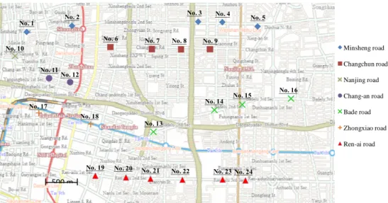
To model traffic flow forecasting for urban arterials, we selected a study area of 5 km by 4 km in Taipei city, Taiwan, and traffic data from 24 vehicle detectors for the westbound traffic were collected. The study area and locations of the sites are displayed in Fig. 1, and the VD No. and the corresponding Station ID are shown in Table I. The attributes of the detectors are available in the webpage of the traffic control center of Taipei city

6

(http://tms.bote.taipei.gov.tw/). Traffic data, including traffic volume, speed and occupancy, were recorded every 5 minutes. Since there are traffic signals in the urban area with cycle length of approximately three minutes, the variability of the traffic flow within a short time is strong. Therefore, the 5-min data are aggregated into 15-min intervals in the analysis, and there are 96 observations each day.

Data sets were collected since 29th June 2009 for four weeks, and the data shows daily and weekly seasonal pattern. The data of the first nine days are used for estimation of the model parameters, and the data of the following day are used for validation and demonstration of the model forecasting performances. As the proposed models require that the data to be no missing, occasional missing values are interpolated with the immediate before and after values in the time series.

B. Modeling with Seasonal ARIMA

A prior study [14] by the authors using the same set of data determined that (2, 0, 1)×(0, 1, 1)96 is a better model with smaller estimation and forecasting discrepancies, and the resultant model is a linear recursive estimator

(

) (

)

( )96 96 1 ( )96 97 1 1 98 2 2 97 1 1 96 ˆ − − − − − − − − + − − − + − + = t t t t y t y t t y y y y y y ε θ θ ε θ ε θ φ φ (14)

where yˆ_t and y_t are the forecasted and observed flow values at time t.

C. Modeling with STARIMA

Traffic characteristics and network topology are incorporated into the spatial modeling by defining a hierarchical structure for the neighboring relationships of the locations of the detectors. The first order and second order neighbors for each detector are defined in Table I, and the corresponding weighting matrices are determined with (10). To identify the tentative model, we examine the pattern of the space-time sample autocorrelations and partial autocorrelations, which are calculated as in Table II. The sample autocorrelations indicate that there is a spike at spatial lag 0 and temporal lag 96 for the seasonal order. At the non-seasonal level, the magnitudes of values seem to be large at time lag 2 for spatial lags 0. The corresponding moving average terms are included in the model tentatively. The sample partial autocorrelations also indicate that there is a spike at spatial lag 0 and temporal lag 96 for the seasonal order and a cut off at time lag 2 for the non-seasonal order, and we include these terms in the autoregressive part.

Various combinations of the parameters are experimented, and it is an iterative process to identify, estimate and reformulate the model. The final model is

( )

( )

(

)

( )

_{( )}

( )

₍

₎

₍

₎

( )

(

t

) ( )

t t t t t t t ε ε ε z W z W z z z + − − − − − + − + − + − = 96 2 2 1 2 1 0 96 0 2 2 22 1 11 20 10 θ θ φ φ φ φ (15)

7

and the estimated parameters are displayed in Table IIIIII. The p-values of all parameters are less than 0.01, indicating that the selected model is suitable to describe the data. The space-time autocorrelations and partial autocorrelations of the residuals are insignificant. Therefore, the final model passes the diagnostic checking.

In the final model, the estimated parameters show a desired structure. The chosen parameters are quite similar to the seasonal ARIMA, with AR terms at non-seasonal level and MA terms at both non-seasonal and seasonal level. For traffic flow forecasting, it is reasonable to expect AR terms with spatial lags because traffic flows progress from upstream to downstream, whereas the MA terms have no spatial lag since the errors are not transferred between measurement sites. Furthermore, at spatial lag 0, the coefficients of the AR terms are decreasing over the time lag. For spatial lag 1, φ₁₁ is significant and φ₂₁ is insignificant, implying that the traffic at a location is affected by its close neighbors at a shorter time lag. In contrast, for spatial lag 2, φ₁₂ is insignificant and φ₂₂ is significant, and it means that the effect due to the neighbors further apart appears at a longer time lag. In addition, φ₁₁ has a higher value than φ₂₂, as neighbors closer in space and time should have a stronger effect than neighbors further away in space and time. Since the parameters are meaningful, we conclude that the selected model is suitable to describe the data and will be used for the forecasting purpose.

D. Forecasting and Comparisons

We compare the forecasting performances of the ARIMA and STARIMA models. The discrepancies between the modeled and observed time series are measured by Root Mean Square Error (RMSE) and Mean Absolute Percentage Error (MAPE). The data of one day (i.e. 96 observations) are used for the validation purpose. Selected time series (VD Nos.1 – 6) are compared in Fig. 2. In overall, the forecasting ability of STARIMA model is comparable to and better than that of the univariate ARIMA models. The average RMSE and MAPE are 40.88 (veh./15 mins) and 15.83% respectively for the STARIMA model, which are reasonably good for urban traffic forecasting (and the MAPE is 11.91% if we evaluate the 6am-6pm time intervals).

V. CONCLUSIONSANDRECOMMENDATIONS

In this paper, a space-time and multivariate technique is introduced to model the spatial and temporal dependences of traffic flows at different locations in an urban network. The space-time autoregressive integrated moving average (STARIMA) model, which is an extension of the univariate ARIMA model, is proposed and the solution approach is described. As compared to the ARIMA model, the advantage of STARIMA is that the traffic conditions of various locations in the network which are expected to exhibit spatial relationships can be formulated as a single model. The final model shows a relative simple structure and offers a large reduction in the number of parameters to be estimated.

8

計劃成果自評：

論文已經投稿，現正第二次審查當中，以上文章為 10 頁的精簡版。

Wong, K.I. and Hsieh, Ya-Chen (2011) A Space-Time Approach to the Short-Term Traffic Flow Forecasting for Urban Roads, IEEE Transactions on Intelligent Transportation Systems. (submitted)

REFERENCES

[1]  B.  Ghosh,  B.  Basu,  and  M.  O'Mahony,  "Multivariate  Short‐Term  Traffic  Flow  Forecasting  Using  Time‐Series  Analysis,"  IEEE  Transactions  on  Intelligent  Transportation Systems, vol. 10, pp. 246‐254, 2009. 

[2]  Y.  Yue  and  A.  G.‐O.  Yeh,  "Spatiotemporal  traffic‐flow  dependency  and  short‐term  traffic  forecasting,"  Environment  and  Planning  B:  Planning  and  Design,  vol.  35,  pp.  762‐771, 2008. 

[3]  T. Cheng, J. Haworth, and J. Wang, "Spatio‐temporal autocorrelation of road network  data," Journal of Geographical Systems, pp. 1‐25, 2011. 

[4]  B.  M.  Williams  and  L.  A.  Hoel,  "Modeling  and  forecasting  vehicular  traffic  flow  as  a  seasonal  ARIMA  process:  Theoretical  basis  and  empirical  results,"  Journal  of  Transportation Engineering‐Asce, vol. 129, pp. 664‐672, Nov‐Dec 2003. 

[5]  B.  L.  Smith,  B.  M.  Williams,  and  R.  Keith  Oswald,  "Comparison  of  parametric  and  nonparametric  models  for  traffic  flow  forecasting,"  Transportation  Research  Part  C:  Emerging Technologies, vol. 10, pp. 303‐321, 2002. 

[6]  B.  L.  Bowerman  and  R.  T.  O'Connell,  Forecasting  and  Time  Series:  An  Applied  Approach, 1993. 

[7]  E.  Vlahogianni,  J.  C.  Golias,  and  M.  G.  Karlaftis,  "Short‐term  traffic  forecasting:  Overview of objectives and methods," Transport Reviews, vol. 24, pp. 533‐557, 2004.  [8]  P.  E.  Pfeifer  and  S.  J.  Deutsch,  "A  Three‐Stage  Iterative  Procedure  for  Space‐Time 

Modeling," Technometrics, vol. 22, pp. 35‐47, 1980. 

[9]  H. Lütkepohl, Forecasting Aggregated Vector ARMA Processes: Springer, 1987. 

[10]  Y.  Kamarianakis  and  P.  Prastacos,  "Space‐time  modeling  of  traffic  flow,"  Comput.  Geosci., vol. 31, pp. 119‐133, 2005. 

[11]  R. L. Martin and J. E. Oeppen, "The identification of regional forecasting models using  space‐time correlation functions," Transactions of the Institute of British Geographers,  vol. 66, pp. 95‐118, 1975. 

[12]  SAS, v9.2, SAS Institute Inc. www.sas.com, 2009. 

[13]  C.  F.  Ansley  and  R.  Kohn,  "A  Note  on  Reparameterizing  a  Vector  Autoregressive  Moving  Average  Model  to  Enforce  Stationarity,"  Journal  of  Statistical  Computation  and Simulation, vol. 24, pp. 99‐106, 1986. 

9

Proceedings  of  the  14th  International  Conference  of  the  Hong  Kong  Society  for  Transportation Studies, Hong Kong, 2009, pp. 779‐788. 

No. 1 No. 2

No. 3 No. 4 _{No. 5}

No. 6 _{No. 7 No. 8 No. 9} No. 10 No. 11 No. 12 No. 13 No. 14 No. 15 No. 16 No. 17 No. 18

No. 19 No. 20 _{No. 21 No. 22 No. 23 No. 24}

Minsheng road Changchun road Nanjing road Chang-an road Bade road Zhongxiao road Ren-ai road

Fig. 1. Locations of the vehicle detectors in the study area in Taipei city, Taiwan   0 50 100 150 200 250 300 350 0 12 24 36 48 60 72 84 96 T raf fi c V ol u m e ( ve h ./15-mi n) Time Interval VMTG520 (VD No.1) Observation Seasonal ARIMA Space-time ARIMA 0 50 100 150 200 250 300 350 400 450 500 0 12 24 36 48 60 72 84 96 T ra ff ic V ol u m e (v eh ./1 5-m in ) Time Interval VMXH820 (VD No.2) Observation Seasonal ARIMA Space-time ARIMA 0 100 200 300 400 500 600 700 800 900 0 12 24 36 48 60 72 84 96 T ra ff ic V ol u m e (v eh ./1 5-m in ) Time Interval VMZL960 (VD No.3) Observation Seasonal ARIMA Space-time ARIMA 0 100 200 300 400 500 600 700 800 0 12 24 36 48 60 72 84 96 T ra ff ic V ol u m e (v eh ./1 5-m in ) Time Interval VMZLI20 (VD No.4) Observation Seasonal ARIMA Space-time ARIMA

Fig. 2. Observed traffic flow and the forecasting using seasonal ARIMA and Space-time ARIMA

Table I

Spatial neighboring relationships of the vehicle detectors

No. Station ID 1st order

2nd

order No. Station ID 1st order 2nd order

1 VMTG520 2 6 13 VJTJ960 14,15 16

10 2 VMXH820 3 6 14 VKLLH20 15,16 9 3 VMZL960 4,5 9 15 VKRM820 16 - 4 VMZLI20 5 - 16 VKWNV20 - - 5 VMYN820 - - 17 VKLGD20 18 11 6 VMFIG20 7,8 9 18 VKAHN20 - 13,19 7 VMDL820 8,9 3 19 VIRHZ20 20,21 22 8 VMEKD00 9 3,14 20 VIPIZ60 21,22 23 9 VMDL800 - 4,15 21 VIPJA20 22,23 24 10 VM7FI60 - 1,11 22 VINKW20 23,24 - 11 VLKGF40 12 6 23 VINLD61 24 - 12 VLGGY60 - 6 24 VINM760 - - Table II

Space-time autocorrelations and partial autocorrelations of the differenced time series

Space-time autocorrelations Space-time partial autocorrelations Time lag

(s)

Spatial lag (l) Time lag (s) Spatial lag (l) 0 1 2 0 1 2 1 0.2403 0.0714 0.0320 1 0.2349 0.0067 0.0132 2 0.1418 0.0796 0.0135 2 0.0807 0.0433 -0.0077 3 0.0271 0.0095 0.0045 3 -0.0245 -0.0197 -0.0011 4 0.0666 0.0559 0.0072 4 0.0521 0.0366 -0.0009 … … 96 -0.4097 -0.0975 -0.0078 96 -0.3901 0.0147 0.0198 Table III

Estimated parameters of the final STARIMA model

Parameter Estimate Std.

Error t-value p-value

10 φ 0.2576 0.0057 45.43 <.0001 11 φ 0.0295 0.0073 4.05 <.0001 20 φ 0.0294 0.0094 3.14 0.0018 22 φ 0.0200 0.0068 2.95 0.0033 20 θ 0.0312 0.0074 4.22 <.0001 96 θ -0.6655 0.0046 -143.42 <.0001

出席國際學術會議心得報告

計畫編號 NSC 99 - 2221 - E - 009 - 094 計畫名稱 時空關聯之市區短期交通預測模式 出國人員姓名 服務機關及職稱 黃家耀 助理教授, 國立交通大學, 運輸科技與管理學系

會議時間地點 11-14 December 2010, Hong Kong

會議名稱 The 15

th

International Conference of the Hong Kong Society for Transportation Studies (HKSTS)

發表論文題目 Short-term traffic flow forecasting for urban roads using Space-time ARIMA 會議時間地點 15-17 December 2010, Hong Kong

會議名稱 The First International Conference on Sustainable Urbanization (ICSU)

發表論文題目 On the path towards sustainable transportation for gaming-led tourism city: the case of Macao

會議時間地點 19-27 June 2011, Jeju, Korea

會議名稱 The 9th Eastern Asia Society for Transportation Studies (EASTS) 發表論文題目 Modeling household car and motorcycle ownership: a case of Macao. With the sponsorship of the National Science Council, I have attended the 15th International Conference of the Hong Kong Society for Transportation Studies (HKSTS) and the First International Conference on Sustainable Urbanization (ICSU) in Hong Kong. The two conferences are back-to-back, and HKSTS is the annual international conference in the transportation area. The papers were presented in the conference.

I have also attended the The 9th Eastern Asia Society for Transportation Studies (EASTS) conference in Jeju, Korea for paper presentation. This biennium conference is a main

gathering of academics from Asian countries. Participants were mainly from Taiwan, Japan, Korea, China, Hong Kong, Thailand, Indonesia etc. It was a good chance to meet people for discussions, and the discussions with experts in the area have sharpened my idea in research. Extended version of the paper has been submitted for possible journal publication and is currently under review.

Copies of the abstracts are attached for reference.

Publications:

1. Wong, K.I. and Hsieh, Ya-Chen (2010) Short-term traffic flow forecasting for urban roads using Space-time ARIMA. In Proceedings of the 15the International Conference of Hong Kong Society for Transportation Studies (HKSTS), 11-14 December, Hong Kong.

gaming-led tourism city: the case of Macao. In Proceedings of the First International Conference on Sustainable Urbanization (ICSU), 15-17 December, Hong Kong.

3. Wong, K.I. and Lin, Hung-Ling (2011) Modeling household car and motorcycle ownership: a case of Macao. In Proceedings of the Eastern Asia Society for Transportation Studies, Vol.8, 19-23 June, Jeju, Korea.

SHORT-TERM TRAFFIC FLOW FORECASTING FOR URBAN ROADS USING SPACE-TIME ARIMA

K.I. WONGa and YA-CHEN HSIEHb

a,b

Department of Transportation Technology and Management, National Chiao Tung University, Taiwan

Email: kiwong@mail.nctu.edu.tw

ABSTRACT 

With the development of technologies in telemetric, the interests and applications of Intelligent Transportation Systems (ITS) have been growing in the recent years. The applications in Advanced Traveler Information System (ATIS) and Advanced Traffic Management Aystem (ATMS) require the forecasting of traffic pattern to the near future. In contrast to the strategic models which predict over a period of month or year for long-term planning purposes, short-term models forecast traffic conditions within a day or a few hours that capture the dynamics of traffic, and are suitable for traffic management and information systems.

A wide variety of short-term traffic forecasting problems have been investigated during past decades. An earlier comprehensive overview was given by Vlahogianni et al. (2004). Usage of input data would separate the forecasting techniques into univariate and multivariate approaches (Makridakis and Wheelwright, 1978). Univariate methods assumed that utilizing the historical time series data of a single variable is sufficient to detect the basic pattern for forecasting. Among the univariate models, autoregressive integrated moving average (ARIMA) model has been successfully applied in many areas and proved for its advantages over some other forecasting methods (Williams et al., 1998; Smith et al., 2002). Multivariate methods assumed there exists some relationships between two or more variables, and this pattern or trend can be extrapolated into the future (Stathopoulos and Karlaftis, 2003). This approach enables the modeling of the relationship of traffic measurements at different locations.

The modelling of spatial-temporal domain of traffic data in urban area has been receiving attention in the recent years. Yang (2006) developed a spatial-temporal Kalman filter (STKF) forecasting model to compare with ARIMA and neural network (NN). An adaptive forecasting model selection strategy was proposed, which selects STKF with time data, but switch to use historical average method if real-time data was not available. Ghosh et al. (2009) proposed a structural real-time-series model methodology, which considers explicitly the trend, seasonal, cyclical, and calendar variations of traffic pattern, with the model flexibility that the immediate upstream junctions can be incorporated in the model as explanatory variables for the downstream predictions.

In this paper, the space-time ARIMA (STARIMA) is used to investigate the spatial-temporal relationship and forecasting of urban traffic flow. Following the successful implements of ARIMA in the single location traffic prediction, a natural extension is to develop the multivariate version of the model with spatial-temporal domain. The space-time ARIMA model was firstly proposed by Pfeifer and Deutsch (1980), and is characterized by the autoregressive and moving average forms of several univariate time series lagged in both space and time. As compared to the ARIMA model, the calibrated model of STARIMA has the advantage with its small number of parameters, requiring fulfillment of rigorous statistical tests. A case study using the traffic data from 24 vehicle detectors in Taipei city, Taiwan are used to illustrate the performance of the model, and it is shown that STARIMA model are suitable for traffic flows forecasting in urban area.

References

Ghosh, B., Basu, B. & O'Mahony, M. (2009) Multivariate Short-Term Traffic Flow Forecasting Using Time-Series Analysis. IEEE Transactions on Intelligent Transportation Systems, 10, 246-254. Makridakis, S. and Wheelwright, S. C. (1978) Interactive forecasting: univariate and multivariate

methods. San Francisco, CA: Holden-Day.

Pfeifer, P. E. and Deutsch, S. J. (1980) A Three-Stage Iterative Procedure for Space-Time Modeling. Technometrics, 22, 35-47.

Smith, B. L., Williams, B. M. and Oswald, R.K. (2002) Comparison of parametric and nonparametric models for traffic flow forecasting. Transportation Research Part C: Emerging Technologies, 10, 303-321.

Stathopoulos, A. and Karlaftis, M. G. (2003) A multivariate state space approach for urban traffic flow modeling and prediction. Transportation Research Part C: Emerging Technologies, 11, 121-135. Williams, B. M., Durvasula, P. K. and Brown, D. E. (1998) Urban freeway traffic flow prediction:

Application of seasonal autoregressive integrated moving average and exponential smoothing models. Transportation Research Record: Journal of the Transportation Research Board, 1644 132-141.

Vlahogianni, E., Golias, J. C. and Karlaftis, M. G. (2004) Short-term traffic forecasting: Overview of objectives and methods. Transport Reviews, 24, 533-557.

Yang, Y. (2006) Spatial-Temporal Dependency of Traffic Flow and its Implications for Short‐ term Traffic Forecasting. PhD Thesis. Department of Urban Planning & Environmental Management University of Hong Kong.

On the path towards sustainable transportation for gaming-led tourism city: The case of Macao

I.M.Wan1 and K.I.Wong2 1

Department of Civil and Environmental Engineering, University of Macau, Macao SAR, China. Email: imwan@umac.mo

2

Department of Transportation Technology and Management, National Chiao Tung University, Taiwan. Email: kiwong@mail.nctu.edu.tw

ABSTRACT

As one of the two special administrative regions of China, Macao is a gaming-led tourism city owing to its unique city profile. Macao has rich historic buildings and monuments, and the historic center was awarded ‘World Cultural Heritage’ by the United Nations Educational, Scientific and Cultural Organization in 2005. Since reunification with China in 1999, the Macao Government has defined gaming sector as their long term economic development direction and has deregulated the monopoly of the gaming industry in 2002. This strategy has successfully boosted the tourism as well as the economics in the city. However, the transportation system does not catch up with the increasing demand from both citizens and visitors, and the mobility of people within the city is of increasing concern. Notably, casinos and gaming groups provided their own transportation service – free shuttle services between selected locations – to compete between each other. This solves part of the transportation problem for visitors but also damages the accessibility of many local residents in various ways. Recently, the Government has announced the first ten-year land transport policy consultation paper for defining goals towards sustainable transportation development for the next decade. In this study, an overview of transportation system of Macao will be carried out through the assessment of urban development, land use and tourism. The impacts of city development and the possible directions for sustainable transportation of the city will be discussed. The unique experience for a tourism oriented city for developing transport sustainability will be critically examined.

KEYWORDS

Modeling Household Car and Motorcycle Ownership: A Case of Macao

K.I. WONG Assistant Professor

Department of Transportation Technology & Management

National Chiao Tung University 1001 Ta Hsueh Road, Hsinchu, 30010, Taiwan

Fax: +886-(0)3-5720844

Email: kiwong@mail.nctu.edu.tw

Hung-Ling LIN Research Student

Department of Transportation Technology & Management

National Chiao Tung University 1001 Ta Hsueh Road, Hsinchu, 30010, Taiwan

Fax: +886-(0)3-5720844

E-mail: hungling329@gmail.com

Abstract:Reducing the private vehicle ownership and usage is one of the key challenges in the development of a sustainable transportation system. However, to evaluate the

effectiveness of a policy, it is necessary to understand the factors that influence the

preferences and behavior of travelers. In this paper, the characteristics of household vehicle ownership level for cars and motorcycles in Macao are investigated. A discrete choice approach is used to estimate the number of vehicles that a household would own using disaggregate household survey data. The result suggests that income has positive effect on both car and motorcycle ownership. Car ownership level is higher at lower population density at residential location, whereas motorcycle is more popular at high population density area.

國科會補助計畫衍生研發成果推廣資料表

日期:2011/10/30

國科會補助計畫

計畫名稱: 時空關聯之市區短期交通預測模式 計畫主持人: 黃家耀 計畫編號: 99-2221-E-009-094- 學門領域: 交通運輸

無研發成果推廣資料

99 年度專題研究計畫研究成果彙整表

計畫主持人：黃家耀 計畫編號：99-2221-E-009-094-計畫名稱：時空關聯之市區短期交通預測模式 量化 成果項目 實際已達成 數（被接受 或已發表） 預期總達成 數(含實際已 達成數) 本計畫實 際貢獻百 分比 單位 備 註 （ 質 化 說 明：如 數 個 計 畫 共 同 成 果、成 果 列 為 該 期 刊 之 封 面 故 事 ... 等） 期刊論文 0 0 100% 研究報告/技術報告 0 0 100% 研討會論文 1 0 100% 篇 論文著作 專書 0 0 100% 申請中件數 0 0 100% 專利 已獲得件數 0 0 100% 件 件數 0 0 100% 件 技術移轉 權利金 0 0 100% 千元 碩士生 1 0 100% 博士生 0 0 100% 博士後研究員 0 0 100% 國內 參與計畫人力 （本國籍） 專任助理 0 0 100% 人次 期刊論文 1 0 100% 研究報告/技術報告 0 0 100% 研討會論文 1 0 100% 篇 論文著作 專書 0 0 100% 章/本 申請中件數 0 0 100% 專利 已獲得件數 0 0 100% 件 件數 0 0 100% 件 技術移轉 權利金 0 0 100% 千元 碩士生 0 0 100% 博士生 0 0 100% 博士後研究員 0 0 100% 國外 參與計畫人力 （外國籍） 專任助理 0 0 100% 人次

其他成果

(

無法以量化表達之成 果如辦理學術活動、獲 得獎項、重要國際合 作、研究成果國際影響 力及其他協助產業技 術發展之具體效益事 項等，請以文字敘述填 列。) 無 成果項目 量化 名稱或內容性質簡述 測驗工具(含質性與量性) 0 課程/模組 0 電腦及網路系統或工具 0 教材 0 舉辦之活動/競賽 0 研討會/工作坊 0 電子報、網站 0 科 教 處 計 畫 加 填 項 目 計畫成果推廣之參與（閱聽）人數 0

國科會補助專題研究計畫成果報告自評表

請就研究內容與原計畫相符程度、達成預期目標情況、研究成果之學術或應用價

值（簡要敘述成果所代表之意義、價值、影響或進一步發展之可能性）

、是否適

合在學術期刊發表或申請專利、主要發現或其他有關價值等，作一綜合評估。

1. 請就研究內容與原計畫相符程度、達成預期目標情況作一綜合評估

■達成目標

□未達成目標（請說明，以 100 字為限）

□實驗失敗

□因故實驗中斷

□其他原因

說明：

2. 研究成果在學術期刊發表或申請專利等情形：

論文：□已發表 ■未發表之文稿 □撰寫中 □無

專利：□已獲得 □申請中 ■無

技轉：□已技轉 □洽談中 ■無

其他：（以 100 字為限）

論文已經投稿，現正第二次審查當中。

Wong, K.I. and Hsieh, Ya-Chen (2011) A Space-Time Approach to the Short-Term Traffic Flow Forecasting for Urban Roads, IEEE Transactions on Intelligent Transportation Systems. (submitted)

3. 請依學術成就、技術創新、社會影響等方面，評估研究成果之學術或應用價

值（簡要敘述成果所代表之意義、價值、影響或進一步發展之可能性）（以

500 字為限）

在市區的交通管理系統上，交通流量的時空關聯關係是十分重要。大量的文獻都以單變量 的時間序列為研究對象，並不考慮多變量之間的空間關係。本研究提出一空間聯關的交通 流量預測模型，以 STARIMA 模型為基礎，並根據量測點的相對位置建立路網設定的方式。 本研究以台北市一區域為範例分析對象，說明所提出的模型有效表達多個量測點的時間與 空間的相關性。