無線網狀網路下結合多頻道連結層與多路徑路由之協定設計

全文

(1)國立交通大學網路工程研究所碩士論文. 無線網狀網路下結合多頻道連結層與多路徑路由之協定設計 Joint Multi-Channel Link Layer and Multi-Path Routing Design for Wireless Mesh Networks. 研究生：談偉航指導教授：曾煜棋. 中華民國. 教授. 九十五. 年七月.

(2) 無線網狀網路下結合多頻道連結層與多路徑路由之協定設計 Joint Multi-Channel Link Layer and Multi-Path Routing Design for Wireless Mesh Networks. 研究生：談偉航. Student：Wai-Hong Tam. 指導教授：曾煜棋. Advisor：Yu-Chee Tseng. 國立交通大學網路工程研究所碩士論文. A Thesis Submitted to Institute of Network Engineering College of Computer Science National Chiao Tung University in partial Fulfillment of the Requirements for the Degree of Master in. Computer Science July 2006 Hsinchu, Taiwan, Republic of China. 中華民國九十五年七月.

(3) 無線網狀網路下結合多頻道連結層與多路徑路由之協定設計學生：談偉航. 指導教授：曾煜棋教授. 國立交通大學網路工程研究所碩士班. 摘. 要. 近年來，無線網狀網路越來越受矚目，並將成為下一世代的無線寬頻存取技術。但如何增加網路吞吐量仍然公認為一關鍵且極具挑戰性的研究題目。其中一的解決方法是把無線收發器動態地切換到多個無線頻道上，以減少相互之間的干擾。但過往的研究只假設上層使用單一路徑的路由方法，像 AODV 或 DSR 等。而本論文則探討在這種多頻道環境下，使用多重路徑路由以提高其端對端的吞吐量。介於媒體存取控制層和網路層，我們提出了新的網路協定─Joint Multi-channel and Multi-path control (JMM)，它結合了多頻道連結層與多路徑路由的功能。藉由把時間軸切割成很多固定大小的時間槽，JMM 能有效地決定每個時間槽應該停留在哪一頻道上，並把封包合理安排到兩條路徑中。全面把競爭的封包分散到不同的頻道，不同的時間，以至不同的路徑上，以大幅度提升其吞吐量。以我們的認知，此為第一個在無線網狀網路下把多頻道與多路徑路由兩者結合的設計。關鍵字：媒體存取控制、多頻道、多路徑路由、排程、無線網狀網路. i.

(4) Joint Multi-Channel Link Layer and Multi-Path Routing Design for Wireless Mesh Networks Student: Wai-Hong Tam. Advisor: Prof. Yu-Chee Tseng. Institute of Network Engineering National Chiao Tung University. Abstruct In recent years, the wireless mesh network (WMN) attracts the interest of many people as a new broadband Internet access technology. However, increasing throughput is still an open and challenging research issue. One potential solution is to enable transceivers to utilize multiple channels dynamically. However, most of existing works do not consider the routing issue, and trivially use some popular single-path routing protocols like AODV and DSR. In this thesis, we exploit the benefit of multi-path routing in multi-channel WMNs from the aspect of end-to-end throughput. Between medium access control and network layers, we propose a novel protocol named Joint Multi-channel and Multi-path control (JMM) which combines multi-channel link layer with multi-path routing. Dividing the time into slots, JMM coordinates channel usage among slots and schedules traffic flows on dual paths. Our scheme efficiently decomposes contending traffics over different channels, different time, and different paths, and hence leads to significant throughput improvement. To the best of our knowledge, this is the first work discussing the joint design of multi-channel control and multi-path routing for WMNs. Keywords: medium access control, multi-channel, multi-path routing, scheduling, wireless mesh network.. ii.

(5) 誌. 衷心感謝我的指導教授. 謝. 曾煜棋教授這兩年來的諄諄教導，使我在研究態. 度、方法以及專業知識上，獲得很大的啟發；同時也給予我很多難得的機會，例如跟國外學者作交流討論、訓練我寫作專書、參與研討會、執行研究計劃等等，相信這些對於我往後的發展將有非常深遠之影響。還有我的專題指導教授. 鍾崇斌教授，大學導師. 莊榮宏教師，以及. 陳榮. 傑教授，他們平日對我的建議和指導，以及生活上的關懷和問候，亦使我獲益良多，在此也致上由衷的謝意。在研究期間，感謝諸多學長姐的關懷指導。特別是把我引進這篇論文領域的亭佑學姐（以後的稱呼要改成教授了），沒有她當初給我關於多頻道無線網狀網路的引導，相信今天的研究之路不會如此順利。還有威碩、佩曄、炳榕、致宇、和 HSCC 實驗室全體同仁在我研究之路上的提攜、扶持，在此也一併致謝。還要感謝澳門高等教育輔助辦公室提供的研究生獎學金，在經濟上給予很大支持，使我能專注於研究工作，不用為生活而勞累。最後當然要感謝我的父母，和美英。談偉航謹誌於新竹交大公元 2006 年 7 月 18 日. iii.

(6) Contents Abstract (Chinese). i. Abstract (English). ii. Acknowledgements. iii. Contents. iv. List of Tables. vi. List of Figures. vii. 1 Introduction. 1. 1.1. Contributions . . . . . . . . . . . . . . . . . . . . . . . . . . . . . . . . . .. 3. 1.2. Organization of the Thesis . . . . . . . . . . . . . . . . . . . . . . . . . . .. 3. 2 Motivation. 4. 2.1. Single-Channel, Single-Path (SCSP) Scenario . . . . . . . . . . . . . . . .. 4. 2.2. Multi-Channel, Single-Path (MCSP) Scenario . . . . . . . . . . . . . . . .. 6. 2.3. Single-Channel, Multi-Path (SCMP) Scenario . . . . . . . . . . . . . . . .. 7. 2.4. Multi-Channel, Multi-Path (MCMP) Scenario . . . . . . . . . . . . . . . .. 7. 3 Related Work 3.1. 9. Multi-Channel MAC and Link Protocols . . . . . . . . . . . . . . . . . . .. 9. 3.1.1. Single-Transceiver Schemes . . . . . . . . . . . . . . . . . . . . . .. 9. 3.1.2. Multi-Transceiver Schemes . . . . . . . . . . . . . . . . . . . . . .. 10. iv.

(7) 3.2. Multi-Channel Routing Protocols . . . . . . . . . . . . . . . . . . . . . . .. 11. 3.3. Multi-Path Routing Protocols . . . . . . . . . . . . . . . . . . . . . . . . .. 12. 4 JMM Protocol. 13. 4.1. Protocol Architecture . . . . . . . . . . . . . . . . . . . . . . . . . . . . . .. 13. 4.2. Multi-Channel Link Layer Part . . . . . . . . . . . . . . . . . . . . . . . .. 14. 4.2.1. Superframe Structure . . . . . . . . . . . . . . . . . . . . . . . . .. 14. 4.2.2. Transmitting and Receiving Patterns . . . . . . . . . . . . . . . . .. 16. 4.2.3. Dynamic Adjustment of the T/R Ratio . . . . . . . . . . . . . . .. 17. 4.2.4. Permutation of Slots . . . . . . . . . . . . . . . . . . . . . . . . . .. 19. 4.2.5. Packet Queues . . . . . . . . . . . . . . . . . . . . . . . . . . . . .. 20. Multi-Path Routing Part . . . . . . . . . . . . . . . . . . . . . . . . . . . .. 20. 4.3.1. Selection of Receiving Channels . . . . . . . . . . . . . . . . . . .. 21. 4.3.2. Dual-Path Route Discovery . . . . . . . . . . . . . . . . . . . . . .. 21. 4.3.3. Path Selection Metric . . . . . . . . . . . . . . . . . . . . . . . . . .. 24. 4.3.4. Determining Superframe Patterns . . . . . . . . . . . . . . . . . .. 25. 4.3.5. Packet Forwarding Rule . . . . . . . . . . . . . . . . . . . . . . . .. 28. 4.3.6. Route Maintenance . . . . . . . . . . . . . . . . . . . . . . . . . . .. 28. 4.3. 5 Performance Evaluation. 30. 5.1. Comparison of SCSP, SCMP, MCSP, and MCMP Routing . . . . . . . . .. 32. 5.2. Impact of Traffic Load . . . . . . . . . . . . . . . . . . . . . . . . . . . . .. 34. 5.3. Impact of Slot Size l on JMM Protocol . . . . . . . . . . . . . . . . . . . .. 34. 5.4. Impact of Available Channels on JMM Protocol . . . . . . . . . . . . . . .. 36. 6 Conclusions. 37. References. 38. v.

(8) List of Tables 1. Spatial reuse factor k in a chain topology. . . . . . . . . . . . . . . . . . .. 5. 2. Structure of the GREQ message (S is the source node). . . . . . . . . . . .. 22. 3. The default parameters in our simulations. . . . . . . . . . . . . . . . . .. 31. vi.

(9) List of Figures 1. The two-tier architecture of wireless mesh networks. . . . . . . . . . . . .. 2. 2. An ideal packet scheduling in the SCSP scenario. . . . . . . . . . . . . . .. 5. 3. An ideal packet scheduling in the MCSP scenario. . . . . . . . . . . . . .. 6. 4. An ideal packet scheduling in the SCMP scenario. . . . . . . . . . . . . .. 7. 5. An ideal packet scheduling in the MCMP scenario. . . . . . . . . . . . . .. 8. 6. The JMM protocol architecture. . . . . . . . . . . . . . . . . . . . . . . . .. 14. 7. The superframe structure. . . . . . . . . . . . . . . . . . . . . . . . . . . .. 15. 8. An example of channel schedule. . . . . . . . . . . . . . . . . . . . . . . .. 16. 9. The TF and RF patterns. . . . . . . . . . . . . . . . . . . . . . . . . . . . .. 17. 10. Four types of superframe patterns. . . . . . . . . . . . . . . . . . . . . . .. 17. 11. A simple slot assignment in a chain of nodes. . . . . . . . . . . . . . . . .. 18. 12. An example reordering slots by the permutation {1, 5, 9, 13, 10, 6, 14, 2, 7, 15, 3, 11, 16, 4, 12, 8}. . . . . . . . . . . . . . . . . . . . . . . . . . . . . .. 19. 13. The broadcast and unicast queues at the link layer. . . . . . . . . . . . . .. 20. 14. A channel selection example. . . . . . . . . . . . . . . . . . . . . . . . . .. 21. 15. The GREQ propagation procedure of a non-gateway node. . . . . . . . .. 23. 16. A GREQ propagation example. . . . . . . . . . . . . . . . . . . . . . . . .. 24. 17. The pattern selection of S when (a) | P1 | − | P2 | is even and (b) | P1 | − | P2 | is odd. . . . . . . . . . . . . . . . . . . . . . . . . . . . . . . . . . . . . . .. 26. An example where the contended link B-S on slave path (..., X, Y, B, S) serves as a link on the master path (..., I, J, B, S, K). . . . . . . . . . . . . .. 27. Protocol stacks of normal and JMM nodes in NCTUns. . . . . . . . . . .. 30. 18. 19. vii.

(10) 20. Structure of our JMM module in the NCTUns simulator. . . . . . . . . .. 32. 21. Single-path and dual-path topologies used in our simulation. . . . . . .. 33. 22. (a) Average end-to-end throughput vs. number of hops, and (b) average end-to-end throughput vs. distance V (path length = 6) . . . . . . . . . .. 33. Aggregate gateway throughput vs. traffic load under different numbers of traffic sources. . . . . . . . . . . . . . . . . . . . . . . . . . . . . . . . .. 35. 24. Aggregate network throughput vs. slot size l. . . . . . . . . . . . . . . . .. 35. 25. Aggregate network throughput vs. number of available channels. . . . .. 36. 23. viii.

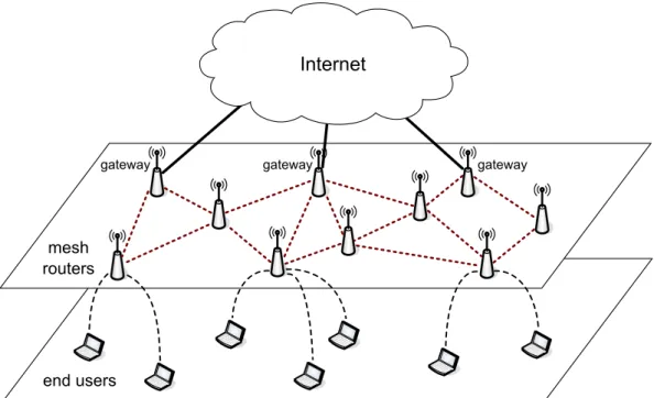
(11) C HAPTER 1. Introduction Wireless Mesh Networks (WMNs) are believed to be a promising technology to offer broadband wireless access to the Internet and to build self-organized networks in places where wired infrastructure is not available or not worthy to deploy [3]. A WMN consists of a collection of wireless mesh routers, which are able to self-configure themselves as a backbone and also serve as an access network to offer connectivity to end-users by standard radio interfaces like 802.11 [1]. A WMN typically has a two-tier architecture as shown in Figure 1. On one hand, mesh routers self-organize themselves to form a wireless backbone, providing large coverage, connectivity, and robustness in the wireless domain. On the other hand, each mesh router is responsible of forwarding traffic on behalf of all end-users in its coverage area. A logical separation is maintained between links connecting end-users and links forming the wireless backbone. One or more mesh routers with wired connections will serve as gateways to provide Internet access. While benefiting from large coverage of multihop wireless connections, WMNs also inherit some of scalability problems in terms of throughput, delay, and packet delivery ratio faced by all multihop wireless networks [11]. Previous studies have shown that end-to-end throughput of a flow may decrease rapidly as the number of hops increases [19, 31]. The main reasons are as follows:. • Half-duplex property of the radios: Radios cannot transmit and receive at the. 1.

(12) Figure 1: The two-tier architecture of wireless mesh networks.. same time. As a result, the capacity of relay nodes is halved. • Broadcast nature of the wireless medium: When all nodes operate at a common communication channel, each node has to compete with neighboring nodes within extended hops, leading to a high collision probability as the traffic load increases. • Difficulty of collision avoidance: In a multihop environment, the common phenomena of hidden and exposed terminals cause collision and unfairness, resulting in reduction of throughput.. There are several approaches to relieving the contention and collision problem, such as using directional antennas, implementing transmission power control, and employing multiple channels. In this thesis, we look for a more cost-effective solution by exploiting multiple non-overlapping channels using only one transceiver per host. While our goal is to improve network performance, we observe that using multiple channels alone is not very effective. Frequency diversity has to be exploited in concert with spatial and temporal reuse. We propose a protocol named Joint Multi-channel and Multi-path control (JMM), which can yield a significant performance improvement by. 2.

(13) decomposing the contending traffic over different channels, different time, and different paths. Our protocol has a great potential to be employed in existing systems because it does not require any changes to the 802.11 standard.. 1.1 Contributions The primary contributions of this thesis can be summarized as follows:. • We first point out that multi-path routing has to be used in concert with multichannel design to improve end-to-end throughput. However, using single-path routing cannot achieve this goal. • We introduce a novel protocol which combines multi-channel link layer with multi-path routing. This protocol is able to increase end-to-end throughput by decomposing the traffic over different channels, time, and space. • In the route discovery phase of our multi-path routing protocol, we propose a GREQ forwarding strategy to reduce the number of broadcast messages. A new routing metric which explicitly accounts for the disjointness between paths and interference among links is proposed. According to this metric, it is easy to select two maximally disjoint paths with less interference.. 1.2 Organization of the Thesis In Chapter 2, we compare single-path routing with multi-path routing in both singlechannel and multi-channel environments to motivate our work. Chapter 3 reviews related work. The proposed JMM protocol is introduced in Chapter 4. Chapter 5 presents our simulation results obtained from NCTUns network simulator. Finally, Chapter 6 concludes the thesis.. 3.

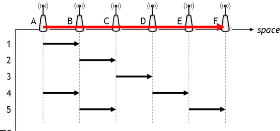
(14) C HAPTER 2. Motivation To motivate the problem, we first observe the upper bounds of end-to-end throughputs under (i) single-channel, single-path, (ii) multi-channel, single-path, (iii) singlechannel, multi-path, and (iv) multi-channel, multi-path scenarios. We show that the multi-channel, multi-path case can achieve better performance.. 2.1 Single-Channel, Single-Path (SCSP) Scenario The most common combination is to use a single-channel MAC protocol like IEEE 802.11 with a single-path routing protocol like AODV (Ad-hoc On demand Distance Vector) [24] or DSR (Dynamic Source Routing) [15]. In this case, packets travel along a chain of nodes toward their destinations. Successive packets on a single chain may interfere with each other as they move along, thus forcing contention in the MAC protocol. This section examines the achievable end-to-end throughput of a single chain. In the SCSP scenario, we show that an ideal protocol could only achieve an end-to-end throughput at most. 1 3. of the effective MAC layer data rate. Consider the network in. Figure 2, where node A is the source and F is the sink. Assume for the moment that radios of nodes that are not neighbors do not interfere with each other. At time 1, node A transmits the first packet to node B. At time 2, nodes A and B cannot transmit at the same time because node B cannot receive and transmit simultaneously. At time 3,. 4.

(15) Figure 2: An ideal packet scheduling in the SCSP scenario. Table 1: Spatial reuse factor k in a chain topology.. Data rate (Mbps). 1. 2. 5.5. 11. S0 (dB). 11. 14. 18. 21. k. 3.4. 4.2. 5.7. 7.2. nodes A and C cannot transmit at the same time because node B cannot correctly hear A while C is sending. At time 4, nodes A and D can send at the same time with the above assumption. Thus, a node can only send. 1 3. of the time.. However, if one assumes that radios can interfere with each other beyond the range at which they can communicate successfully, the situation is even worse. For example, in 802.11b, the interference range is about twice that of transmission range. Hence, in Figure 2, node D’s transmission will interfere with that from A to B. This may reduce a node’s transmission opportunity to. 1 4. of the time.. References [13, 34] investigate this spatial reuse effect from a physical layer perspective. Let k denote the minimum transmitter-transmitter distance (also called spatial reuse factor) in number of hops. Then the lower bound of k is · µ ¶ ¸1 γ 1 k = 2 1+ S0 , γ−1 where S0 denotes the Signal-Noise-Interference Ratio (SNIR) threshold and γ is the pathloss exponent indicating how quickly the RF signal decays as distance inreases. Table 1 shows the values of k for 802.11b under different data rates. As can be seen, the prediction is even more pessimistic.. 5.

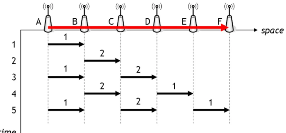
(16) Figure 3: An ideal packet scheduling in the MCSP scenario.. 2.2 Multi-Channel, Single-Path (MCSP) Scenario The above analysis shows the impact due to the broadcast nature of wireless medium. To improve the end-to-end throughput, a lot of researchers have proposed multi-channel solutions. Allowing each transceiver to switch among different channels, instead of waiting in the same channel, the MAC protocol has to deal with channel selection and the multi-channel hidden terminal problems [27]. This section examines the achievable end-to-end throughput of an ideal multi-channel MAC protocol under a chain topology. In the MCSP scenario, we show that an ideal multi-channel MAC protocol could achieve end-to-end throughput as high as. 1 2. of the effective MAC data rate. Consider the sce-. nario in Figure 3. Assume that the MAC protocol can always select an appropriate channel and schedule packets perfectly. At time 1, node A transmits the first packet to node B on channel 1. At time 2, nodes A and B cannot transmit at the same time because node B cannot receive and transmit simultaneously. At time 3, nodes A and C can send at the same time since they use different channels. We can see that if the MAC protocol can switch channels perfectly, node A can continuously inject one packet every other slot. This leads to the factor of 12 . Because of the half-duplex property of radios, the bottleneck appears in the intermediate nodes.. 6.

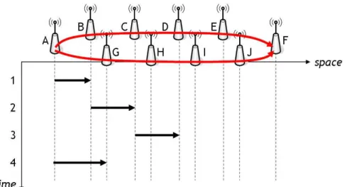
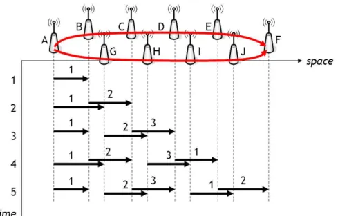
(17) Figure 4: An ideal packet scheduling in the SCMP scenario.. 2.3 Single-Channel, Multi-Path (SCMP) Scenario In this SCMP scenario, packets are split along two disjoint paths leading toward destinations. This section examines its achievable end-to-end throughput. We will show that the broadcast nature of wireless medium may degrade throughput significantly. In fact, the SCMP scenario can only achieve an end-to-end throughput slightly higher than the SCSP scenario. Consider the network in Figure 4, where there are two disjoint paths from source A to destination F. At time 1, node A transmits the first packet along the upper path to node B. At time 2, only one of nodes A and B can transmit because they are competitors. We suppose that B wins in the contention. At time 3, node A can not transmit on the lower path because C will interfere the reception of G. So A can only transmit on the lower path at time 4. So A can only inject a packet every three slots.. 2.4 Multi-Channel, Multi-Path (MCMP) Scenario Some may believe that the factor of. 1 2. is the best case. Below, we show that using a. multi-channel MAC protocol combined with a multi-path routing protocol can overcome the bottleneck at intermediate nodes. In the MCMP scenario, we show that the. 7.

(18) Figure 5: An ideal packet scheduling in the MCMP scenario.. ideal MAC end-to-end throughput can be as high as the effective MAC data rate. Consider the network in Figure 5. Assume that the routing protocol can split packets properly and the MAC protocol can perform ideal channel switching and scheduling. At time 1, node A transmits a packet along the upper path to node B on channel 1. At time 2, node A transmits a packet along the lower path to node G. At the same time node B can transmit along the upper path because they use different channels. Afterward, A can alternate between these two paths in every slot. This concludes out derivation.. 8.

(19) C HAPTER 3. Related Work In the literature, a lot of efforts have been dedicated to multi-channel link protocols and multi-path routing protocols. However, these link layer protocols and routing protocols are investigated separately. This motivates us to design a joint protocol which combines these two approaches. Below, we review the related work in this field.. 3.1 Multi-Channel MAC and Link Protocols Multi-channel link/MAC protocols have been investigated in [2, 4–7, 14, 23, 27, 30, 32, 34]. These works focus on how to utilize multiple channels to reduce the contention and collision among stations. Depending on the number of radio interfaces per node, such protocols can be classified as single-transceiver schemes [4–7, 14, 27, 32] and multitransceiver schemes [2, 23, 30, 34].. 3.1.1 Single-Transceiver Schemes For a single-transceiver system, the radio interface in each node needs to switch among channels. It may result in the multi-channel hidden-terminal problem [27]. The Multichannel MAC (MMAC) protocol [27] proposes to embed a negotiation phase in the ATIM (Ad Hoc Traffic Indication Map) window that is periodically send under the. 9.

(20) Power Save Mode (PSM). During the ATIM window, a predefined common channel is used for all nodes having packets to transmit to negotiate with their destinations. After the ATIM window, nodes may select different channels to transmit and receive packets. The Slotted Seeded Channel Hopping (SSCH) mechanism [4] divides the time axis into virtual channels. The hopping sequence of each virtual channel is determined by a (channel, seed) pair. Whenever a sender wants to communicate with a neighbor, it changes some of its hopping schedules to the receiver’s corresponding virtual channels. SSCH requires a looser time synchronization than [27], but it has a higher channel switching overhead. The Multi-channel coordinated Temporal Topology control (MOTTO) [32] also divides the time axis into epochs. Two continuous epochs are defined, as a cycle, one for uplink channel and the other for downlink channel. The active channel of an epoch is determined statically by the node’s hop-count to a gateway and its direction (uplink or downlink). By controlling the network’s temporal topology through coordinated channel assignments, MOTTO decomposes multihop contending traffic into multiple channels.. 3.1.2 Multi-Transceiver Schemes Dynamic Channel Assignment (DCA) [30] is a multi-channel MAC protocol using two transceivers, one dedicated to transmitting control packets and the other dedicated to transmitting data packets. The first transceiver always operates in a dedicated channel for transmitting RTS/CTS control packets, and the second transceiver may switch among several available data channels. The sender includes in its RTS packet a list of preferred channels. The receiver then chooses a channel and includes the information in its CTS packet. Then DATA and ACK packets are exchanged on the agreed data channel.. 10.

(21) A cluster-based two-radio architecture is proposed in [34]. Each node is assumed to have a radio for intra-cluster communication and one for inter-cluster communication. Nodes in the same cluster use the same channel to communicate. This channel is selected by the cluster head based on neighborhood condition. Different clusters might use different channels to reduce interference. Inter-cluster communication is achieved by using a common default channel. The Multi-radio Unification Protocol (MUP) [2] is a link layer protocol. Each node is assumed to have multiple radios, each operating on a specific channel. To send a packet, MUP selects the radio with better channel characteristics to transmit. Although this scheme performs pretty well, it is based on a strong assumption that the number of available channels is equal to the number of radios per node.. 3.2 Multi-Channel Routing Protocols Several works consider utilizing multiple channels at the network layer [10, 12, 16, 25, 26]. These works focus on how to assign channels to a flow and how to find the best path in the multi-channel environments. The Hyacinth architecture [25] proposes a tree-based routing protocol for a multitransceiver multi-channel WMN. From each gateway, a tree is constructed, along which packets are forwarded. Under this tree structure, the interfaces of each node are divided into two subsets. One subset of interfaces are used to communicate with the node’s parent and are thus assigned the same channels as its parent’s channels. The other subset of interfaces are used to communicate with its children and the node is free to choose the least interfered channels according to its neighborhood condition. This selection is started from the root node and is gradually propagated to its child nodes. Reference [12] proposes a CA-AODV protocol that combines channel assignment with AODV [24]. It assumes a system with one control channel and several data channels. 11.

(22) like DCA [30]. All control packets such as RREQ/RREP are transmitted on the control channel, but nodes may use different channels to exchange data packets. From the exchange of RREQ and RREP packets, a source can achieve both route discovery and channel assignment of the flow. A general multi-channel routing protocol can be designed by combining an existing single-channel routing protocol with a new routing metric by taking multi-channel effects into consideration. The WCETT (Weighted Cumulative Expected Transmission Time) metric in [10] is such a metric for routing in multi-radio multi-hop WMNs. With this metric, one can choose a path with a higher throughput.. 3.3 Multi-Path Routing Protocols Recently, multi-path routing in Mobile Ad hoc Networks (MANETs) has received some attention [17, 18, 20–22, 28, 33]. Based on Directed Acyclic Graph (DAG), TORA [22] can support multiple-path routing. However, it does not guarantee disjointness of paths. DSR [15] can also find multiple paths, naturally by its flooding behavior. But sometimes only a small portion of the found path is disjoint. The Split Multipath Routing (SMR) [18] can solve this problem because duplicate RREQs are not dropped, but this is at the cost or more RREQs. AODVM [33] is an extension to AODV for finding reliable routing paths. Duplicate RREQ packets are not discarded by intermediate nodes. Again, the routing overhead is high. AOMDV [20] is also an extension to AODV for computing multiple loop-free and link-disjoint paths. It uses the notion of an "advertised hop count" to guarantee loop-freedom and uses a particular property of flooding to achieve link-disjointness.. 12.

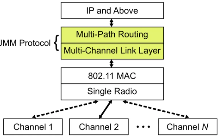
(23) C HAPTER 4. JMM Protocol As reviewed above, all existing investigate multi-path routing and multi-channel MAC separately. This motivates us to design a joint protocol which combines these two strategies together. We present our Joint Multi-channel and Multi-path control (JMM) that can decompose contending traffic over different channels, different time, and different paths to achieve significant throughput improvement.. 4.1 Protocol Architecture The architecture of JMM is shown in Figure 6. Each node is equipped with an offthe-shelf 802.11 wireless adapter with a half-duplex radio which is allowed to switch among different channels and runs the 802.11 MAC protocol. The proposed JMM protocol is a cross-layer design on top of the 802.11 MAC layer and does not require any change to the 802.11 MAC and hardware. It is composed of a multi-channel link layer part and a multi-path routing part. These two parts cooperate with each other tightly. For example, the former needs the distance information from the latter to schedule traffics, which the latter requires the former to provide channel information to select routes. JMM has the following functionalities:. 1. Decide the receiving channel of each node based on neighborhood information (in Section 4.3.1);. 13.

(24) Figure 6: The JMM protocol architecture.. 2. Construct a dual path from each node to its gateway (in Section 4.3.2); 3. Conduct slot assignment for each node’s superframes (in Sections 4.2.2 and 4.3.4); 4. Schedule and forward packets and adjust the ratio of transmitting slots to receiving slots for each node (in Section 4.2.3).. Our presentation is bottom-up, from the link layer part (items 3 and 4) toward the routing part (items 1 and 2).. 4.2 Multi-Channel Link Layer Part The link layer has two functionalities: channel scheduling and packet scheduling. The former is to control which channel the transceiver should stay on, and the latter is to schedule when a packet can be sent. The MAC part follows the IEEE 802.11 standard. Our design will avoid the deafness problem [26] and the multi-channel hidden-terminal problem [27].. 4.2.1 Superframe Structure The time axis is divided into slots of a fixed length l. Slots are organized into superframes. A slot may designated as a transmitting slot or a receiving slot. We will deter-. 14.

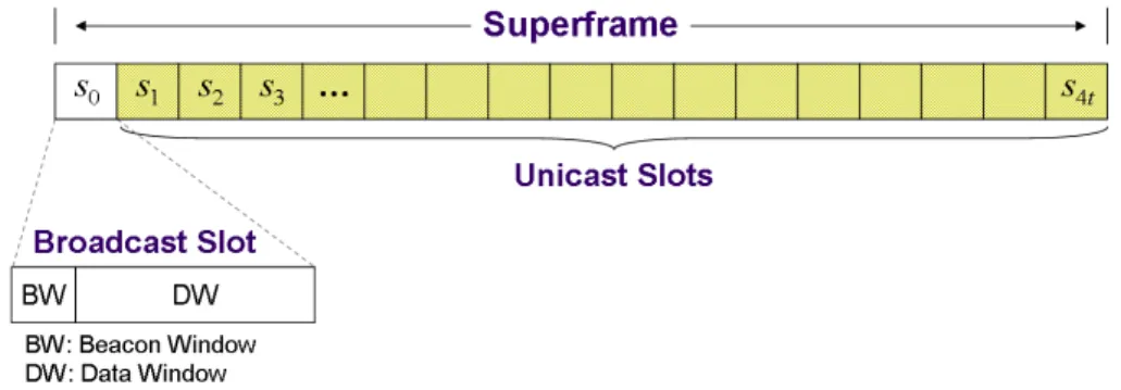
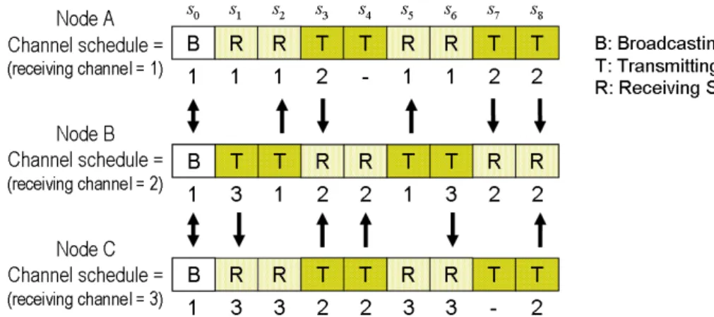
(25) Figure 7: The superframe structure.. mine the channels to be used in slots of a superframe. Our channel assignment strategy is receiver-based. The structure of a superframe is shown in Figure 7. Superframes are loosely synchronized in time. Each superframe comprises 4t + 1 slots, marked as s0 , s1 , ..., s4t , where t is an integer. Slot s0 is a broadcast slot in which only beacons and broadcast messages can be sent. Each broadcast slot is led by a beacon window, followed by a data window. Beacons also serve to synchronize stations’ clocks. To ensure network connectivity, all nodes should stay on a pre-defined common channel in slot s0 . The remaining 4t slots are unicast slots, whose channels will be decided dynamically. The receiver-based channel assignment helps two nodes to switch to the same channel for communication. Unicast slots are designnated as transmitting/receiving slots (refer to Section 4.2.2). A node will select a receiving channel for its receiving slots (refer to Section 4.3.1). Nearby nodes will try to avoid using the same receiving channel. During a receiving slot, a node will stay on its receiving channel. During a transmitting slot, a node can switch to its receiver’s receiving channel and stay on that channel until the end of the slot. Hence, two nodes can communicate only if one is in a transmitting slot and the other is in a receiving slot. After switching to a new channel, a node first remains silent for a duration equals to the maximum packet transmission time so as to avoid the multi-channel hidden terminal problem which is resulted by loose time synchronization. Therefore, JMM does not require very precise clock synchronization. An example is in Figure 8. In s0 , all nodes stay on the common channel 1. In s1 , node B wants to send packets to C, so B switches to C’s receiving channel 3. Suppose that. 15.

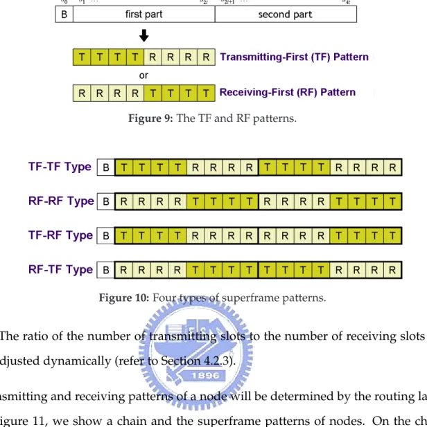
(26) Figure 8: An example of channel schedule.. node A also wants to send packets to B. Since s1 and s2 of node A are receiving slots, it has to wait until s3 to transmit. Note that since both A and C want to send packets to B in s3 , they will use 802.11’s CSMA/CA mechanism to contend for the medium.. 4.2.2 Transmitting and Receiving Patterns Unicast slots of a superframe are designated as transmitting/receiving slots. However, since traffics on mesh networks are quite stable, slot assignment will not be changed too frequently. In each superframe, unicast slots s1 to s4t are evenly divided into two parts, the fist part from s1 to s2t and the second part from s2t+1 to s4t . One part is designated as the upstream part for communication with the node’s upstream nodes (with respect to the node’s gateway), and the other part is called downstream part for communication with its downstream nodes. These two parts are of the same length because for a relay node, the amount of traffics to and from upstream nodes is likely to be equal to that to and from downstream nodes. Each part can follow a Transmitting-First (TF) pattern or a Receiving-First (RF) pattern as shown in Figure 9. In a TF pattern, the first half is all transmitting slots, and the second half is all receiving slots. Contrarily, in a RF pattern, the first half is all receiving slots, and the second half is all transmitting slots. As a result, there are four types of superframe patterns, namely TF-TF, RF-RF, TF-RF, and RF-TF types, as shown in Figure. 16.

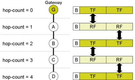
(27) Figure 9: The TF and RF patterns.. Figure 10: Four types of superframe patterns.. 10. The ratio of the number of transmitting slots to the number of receiving slots can be adjusted dynamically (refer to Section 4.2.3). Transmitting and receiving patterns of a node will be determined by the routing layer. In Figure 11, we show a chain and the superframe patterns of nodes. On the chain, packets are alternated between the first and the second halves of superframe. Also on each link, one side if RF pattern and the side is TF pattern. However, with dual paths, slot schedule is more complex than this example (refer to Section 4.3.4).. 4.2.3 Dynamic Adjustment of the T/R Ratio Recall that each superframe has an upstream part and a downstream part. The ratio of the number T of transmitting slots to the number R of receiving slots in each upstream part, call T/R ratio, can be dynamically adjusted in a per node basis. Since in a relay node the amount of traffics from upstream nodes is likely to be equal to that to downstream nodes, the number of receiving slots in the upstream part should equal. 17.

(28) Figure 11: A simple slot assignment in a chain of nodes.. the number of transmitting slots in the downstream part. Similarly, the transmitting slots in the upstream part should equal the number of receiving slots in the downstream part. We thus let T to be the number of receiving slots and R to be the number of transmitting slots in the downstream part. The T/R ratio of each node is adjusted dynamically during runtime. Initially, we set T = R = t. A node should monitor the actual traffic through itself. Assume that the actual transmitting and receiving traffics on the upstream part are Tactual and R actual , respectively. We then compute new weighted averages Tsmooth and Rsmooth as follows: Tsmooth ← α ∗ Tactual + (1 − α) ∗ Tsmooth ;. (1). Rsmooth ← α ∗ R actual + (1 − α) ∗ Rsmooth .. (2). The values of T and R will be changed slowly by the following rules:. 18.

(29) Figure 12: An example reordering slots by the permutation {1, 5, 9, 13, 10, 6, 14, 2, 7, 15, 3, 11, 16, 4, 12, 8}.. if ( Tsmooth /T )/( Rsmooth /R) > Thresholdh and R > 1 then T ← T +1; R ← R−1; endif if ( Tsmooth /T )/( Rsmooth /R) < Thresholdl and T > 1 then T ← T −1; R ← R+1; endif. Tsmooth /T and Rsmooth /R are the utilizations of transmitting and receiving slots, respectively. If the utilization ratio of transmitting to receiving is higher than a thresholds Thresholdh , we increase T and decrease R by one. If the utilization ratio is lower than a threshold Thresholdl , a reverse process is preformed.. 4.2.4 Permutation of Slots In the above discussion, transmitting and receiving slots are clustered togeter. In practice, we can permute the slot sequence of a superframe to obtain some degree of randomness among these slots. The same permutation which can reorder a sequence of 4t elements should be used by all nodes. An example is shown in Figure 12.. 19.

(30) Figure 13: The broadcast and unicast queues at the link layer.. 4.2.5 Packet Queues When packets arrive, we need to allocate them to transmitting slots for transmission. JMM dispatches packets into a broadcast queue and two groups of unicast queues as shown in Figure 13, where we assume that there are three non-overlap channels. Broadcast packets are enqueued in the broadcast queue, while unicast packets are classified as the first part or the second part and then are enqueued in the corresponding queues based on the receiving channels of receivers (refer to Section 4.3.5). The broadcast queue is served in broadcast slots. The first part unicast queues are served by transmitting slots of slots s1 to s2t in a round-robin manner. Each transmitting slot will serve one queue by switching to the channel of that queue, until the queue is empty or the slot expires. The second part unicast queues are served by transmitting slots of slots s2t+1 to s4t in a similar way.. 4.3 Multi-Path Routing Part The goal of the routing part is to construct two paths to the gateway. Since finding the best two paths requires the channel information provided by the link layer part, we. 20.

(31) Figure 14: A channel selection example.. first describe how a node selects its receiving channel. We then present the multi-path route discovery phase and our path selection metric. Finally, we describe our packet scheduling scheme to exploit the benefit of multi-path routing.. 4.3.1 Selection of Receiving Channels When a node is first turned on, it can choose any channel as its receiving channel. Periodically, each node broadcasts its receiving channel to its 2-hop neighbors. This can be achieved by broadcasting a HELLO message carrying a node’s direct neighbors’ receiving channels. Each node maintains a NeighborTable containing the receiving channels of its 2-hop neighbors and a ChannelUsageTable to count the number of nodes using each channel. For example, Figure 14 shows these tables of node A. A node will choose the least used channel as its receiving channel. To prevent unnecessary fluctuation, when a node finds a better channel than its current receiving channel, it will only switch to that channel with a probability p.. 4.3.2 Dual-Path Route Discovery Our goal is to find from each node two paths to its gateway that are as disjoint as possible. However, a dilemma is: on one hand, we would like to avoid network-wide flooding of route search packets, while on the other hand, we would not expect too many duplicate route search packets being discarded by intermediate nodes (otherwise, finding disjoint paths would be difficult).. 21.

(32) Table 2: Structure of the GREQ message (S is the source node).. Field. Initial value. Meanings. seqNum. seq. number at S. the sequence number. srcAddr. S. the source address. gwAddr. unknown. the gateway address of the mesh network. hopCount. ∞. the smallest number of hops to the gateway. pathRecord. {S}. the list of node records on the path. Below, we propose an efficient discovery strategy to find a dual-path to each gateway in the network. A Gateway REQuest (GREQ) packet is used for this purpose. Instead of blindly flooding, limited rebroadcasts of GREQs are invoked. The format of GREQ is shown in Table 2. The route discovery is performed in an incremental way. So when a node issue GREQ, we can assume that each existing node has already established two paths to its gateway. For each node, let gwAddr be its selected gateway and hopCount be the length of the shorter path of its dual-path. When an intermediate node R receives a GREQ message, the procedure in Figure 15 is executed. It first checks whether the sequence number is up-to-date (lines 2-6). Then it verifies if its slot schedule mismatches with that of the transmitter (lines 7-9). Note that a “mismatch” happens when the superframe patterns of two neighboring nodes are the same, in which case these two nodes cannot communicate with each other. The gwAddr and hopCount fields guarantee that the GREQ packet is forwarded toward the gateway indicated in the gwAddr flied and the hopCount value progressively decreases on its way to the gateway (lines 10-19). This forwarding strategy can significantly reduce the rebroadcast overhead while traversing most wireless links. Finally, the node rebroadcasts the GREQ packets (line 20). An example of the GREQ propagation procedure is shown in Figure 16. The links indicated by dashed lines mean that the corresponding GREQ are discarded.. 22.

(33) /*Executed when a non-gateway node R receives a GREQ from a node T */ 01. 02.. begin if GREQ.seqNum < R.seqNum[srcAddr] then. 03. 04.. discard and exit; else R.seqNum[srcAddr] ← GREQ.seqNum;. 05. 06.. endif. 07.. if the slot schedules of R and T mismatch then. 08.. discard and exit;. 09.. endif. 10.. if GREQ.gwAddr 6= unknown and GREQ.gwAddr 6= R.gwAddr then. 11. 12.. discard and exit; endif /* Ensure that hopCount progressively decreases */. 13.. if GREQ.hopCount < R.hopCount then. 14. 15.. discard and exit; elseif GREQ.hopCount = R.hopCount then if R ∈ GREQ.pathRecord then. 16. 17.. discard and exit;. 18.. endif. 19.. endif. 20.. send GREQ(GREQ.seqNum, GREQ.srcAddr, R.gwAddr, R.hopCount, GREQ.pathRecord ∪ {R});. 21.. end Figure 15: The GREQ propagation procedure of a non-gateway node.. 23.

(34) Figure 16: A GREQ propagation example.. 4.3.3 Path Selection Metric After the above procedure, each gateway will collect a number of GREQ packets each carrying a path. Since our goal is to find a dual-path, the gateway will use a metric function to evaluate each pair of paths. For example, the gateway X in Figure 16 will collect n = 4 paths, S-C-A-X, S-D-B-X, S-C-B-X, and S-D-A-X, from the route discovery initiated by S. So there are totally (n+22−1) = 10 path pairs to be evaluated. Note that the combination with repetition is used because a path may serve as both paths of a dual-path in case that there is no good choice. The path pair with the lowest metric will be selected and two Gateway REPly (GREP) packets are unicast along the reverse directions to the source node. Then the source node will collect all GREP packets from different gateways and select the dual-path with the best path metric by sending two GREP ACKnowledgement (GREP_ACK) packets to the selected gateway along the dual-path. The input of the path metric function is a path pair (P1 , P2 ) and the output is a 3tuple V = (Vnode , Vch , Vqlty ). Vnode is the number of common nodes between P1 and P2. 24.

(35) excluding the source node and the gateway. Vch is defined as Vch = CN ( P1 ) + CN ( P2 ) + δ( P1 , P2 ),. (3). where CN ( Pi ) is the number of channel contending pairs along Pi , where two nodes on Pi are called a channel contending pair if they are within 2 hops and use the same receiving channel. For example, CN (S-C-A-X) = 2 because (S, A) and (C, X) are channelcontending pairs. Function δ( P1 , P2 ) = 1 if the difference of the lengths | P1 | and | P2 | is an odd number; otherwise, δ( P1 , P2 ) = 0. The value is so assigned because our algorithm prefers paths differ in lengths by an even number (refer to the discussion in Section 4.3.4). To reflect the signal quality perceived by nodes on P1 and P2 , Vqlty is defined as ETX ( P1 ) + ETX ( P2 ), where ETX ( Pi ) is the expected transmission count of a packet along Pi [8]. Certainly, other metrics for evaluating path quality [9, 10] can be used instead. Given two dual-paths with metrics V = (Vnode , Vch , Vqlty ) and 0 , V 0 , V 0 ), we say that V < V 0 if (i) V 0 0 V = (Vnode node < Vnode , (ii) Vnode = Vnode and ch qlty 0 , or (iii) V 0 0 0 Vch < Vch node = Vnode and Vch = Vch and Vqlty < Vqlty . The one with a lower. metric is preferred.. 4.3.4 Determining Superframe Patterns Next, we need to determine the superframe pattern (TF-TF, RF-RF, TF-RF, or RF-TF type) of each node. The selection will be based on the result of the route discovery. We assume that all nodes on the dual-path except the source have already determined their superframe patterns. Without loss of generality, let the gateway choose the TF-TF type. Given any dual-path, the gateway will designates one path as the master path, and another as the slave path. The requirement to be a master path is that the superframe patterns of the gateway and the first child must match in the first part (i.e. slots s1 to s2t ), and the requirement to be a slave path is that they must match in the second part (slots s2t+1 to s4t ). A “match” happens if one side uses TF and the other side uses RF. Let S be the source, G be the gateway, and ( P1 , P2 ) be the dual-path, such that P1 is the master path and P2 is the slave path. The superframe pattern of S will be selected by 25.

(36) Figure 17: The pattern selection of S when (a) | P1 | − | P2 | is even and (b) | P1 | − | P2 | is odd.. the following rules: (A) | P1 | − | P2 | is even: We refer to Figure 17 for ease of presentation. If | P1 | is odd, the pattern of S’s first part should match with that of its parent on P1 and the pattern of S’s second part should match with that of its parent on P2 . If | P1 | is even, the pattern of S’s first part should match with that of its parent on P2 and the pattern of S’s second part should match with that of its parent on P1 . Hence, S chooses the RF-RF type in Figure 17(a). This pattern selection can achieve high channel utilization. Packets on the dual paths are unlikely to interference with each other because they are separated in both the time domain and the space domain when they happen to use the same channels. (B) | P1 | − | P2 | is odd: In this case, one of | P1 | and | P2 | is odd and the other is even. Let P be the longer path of P1 and P2 . If | P| is odd, the pattern of S’s first part should match with that of its parent on P1 and the pattern of S’s second part should match with that. 26.

(37) Figure 18: An example where the contended link B-S on slave path (..., X, Y, B, S) serves as a link on the master path (..., I, J, B, S, K).. of its parent on P2 . If | P| is even, the pattern of S’s first part should match with that of its parent on P2 and the pattern of S’s second part should match with that of its parent on P1 . Hence, S chooses the RF-TF type in Figure 17(b). In this case, packet transmission on the dual paths are also quite interference-free, except the link between S and its parent on the shorter path of P1 and P2 , which is called the contended link. This is because S matches with its parent on the same part as where S’s parent matches with S’s grandparent on that path. This competition may affect the end-to-end throughput of that path. So we let this happen on the shorter path. Also, the penalty is reflected by the earlier function δ( P1 , P2 ) in the path metric Vch . Note that a contended link may play parts in both a master path of a dual path and a slave path of another dual path. For example, in Figure 18, link B-S is a contended link. If later on node S accepts a child node K, which chooses the path along S as its master path, then this contended link will be part of a master path. As can be seen, the patterns of superframes of K’s master path are not affected by the appearance of contended link.. 27.

(38) 4.3.5 Packet Forwarding Rule With dual-path routing, our system needs to inject packets to both paths to exploit communication parallelism. Below, we summarize our packet forwarding rule. When a source node or a gateway generates a sequence of packets, we will alternately mark them as to be sent along the master path or the slave path. For each packet, we will compute a value P = M ⊕ E ⊕ D ⊕ C for it, where ( 0 if the packet is to be sent along the master path; M = 1 if the packet is to be sent along the slave path; ( 0 if the hop count to gateway along the intended path is even; E = 1 if the hop count to gateway along the intended path is odd; ( 0 if the packet is issued by a gateway; D = 1 if the packet is issued by a source; ( 0 if the packet is to be transmitted to a non-contended link; C = 1 if the packet is to be transmitted to a contended link.. (4) (5) (6) (7). If P = 0, the packet will be forwarded to the first part unicast queues; otherwise, the packet will be sent to the second part unicast queues (refer to Figure 13). For a relayed packet, it is alternated between the first and the second parts except when it passes through a contended link. Specifically, if a packet is received from a contended link, it is enqueued at the same part of unicast queues; otherwise, it is enqueued at a different part of unicast queues from its original. For example, in Figure 17(b), when node B receives a packet from node S in the second part, it enqueues the packet at the same part of unicast queues for transmitting, but when node C receives a packet from S, it enqueues the packet at the different part of unicast queues.. 4.3.6 Route Maintenance Faulty links are detected by nodes’ periodical HELLO messages. Loss a predefined number of HELLOs is an indication of a fault of link. When a node discovers a faulty link, it will propagate a Gateway ERRor (GERR) message to all its successors using. 28.

(39) this link. Each successor will initiate a new gateway discovery procedure to find a new dual-path. Before new paths are found, the other (non-broken) paths can still be used for communication. Therefore, our multi-path routing can also improve the reliability of the WMN.. 29.

(40) C HAPTER 5. Performance Evaluation To evaluate the performance of the proposed protocol, we have implemented a JMM module in the NCTUns network simulator 2.0 [29]. The JMM module has a link layer, a routing layer, and some FIFO queues. Figure 19 compares the protocol stack of a typical node against that of our JMM node. All components described previously are implemented. The MAC layer is the IEEE 802.11a without using RTS/CTS. Data rate is 54 Mbps. Each node has a transmission range of 250 meters and an interference range of 550 meters. The default parameters used are shown in Table 3. The structure of our JMM module is shown in Figure 20. There are mainly seven functional blocks to accomplish routing, forwarding, traffic classification, scheduling, etc. The detail of each functional block is presented as follows.. Figure 19: Protocol stacks of normal and JMM nodes in NCTUns.. 30.

(41) Table 3: The default parameters in our simulations.. Parameter. Default value. Meanings. l. 20 msec. the slot size. t. 4. the number of slots in a quarter of a superfame. α. 0.2. the weight between actual and smooth traffic. Thresholdh. 2. the high threshold of adjusting the T/R ratio. Thresholdl. 0.5. the low threshold of adjusting the T/R ratio. send This function is called when a new packet is generated by the upper layer. It queries the routing table to find the next-hop address using the destination address of the IP header. sendToQueue This function is called by send, relay, and routing. It injects packets into queues. For each packet, the packet forwarding rule in Section 4.3.5 is preformed to determine a group of queues and then the packet is injected into corresponding channel queue based on the default receiving channel of its receiver. chlSwitch This function is called every slot to switch channels according to the node’s superframe pattern by changing the WPhy.channel parameter of the physical layer. intrq This function is called when the previous packet is sent successfully and the lower layer is ready to send the next packet. It dequeues packets based on our algorithm. recv This function receives packets from the lower layer and forwards them to the corresponding component. routing This function manages the multi-path routing protocol and maintains neighbor information. Both GREQ and HELLO messages are processed by this function. relay This function is called when a packet needs to be forwarded to another node. It queries the routing table to find the next-hop address and calls the sendToQueue function to enqueue the packet.. 31.

(42) Figure 20: Structure of our JMM module in the NCTUns simulator.. 5.1 Comparison of SCSP, SCMP, MCSP, and MCMP Routing We first compare the performance of SCSP, SCMP, MCSP and MCMP routing. Network topologies as shown in Figure 21 are tested. Assuming H = 200 meters, V = 300 meters, and five available channels, we vary the number of hops from the gateway to the destination and observe the end-to-end throughput. Continuous 512-byte packets are injected from the gateway to the destination. SCSP routing uses IEEE 802.11 MAC and AODV. SCMP routing uses the multi-path routing protocol AODVM. MCMP routing uses our JMM protocol. MCSP routing also uses our JMM protocol but it only employs a single path routing. The results are shown in Figure 22(a). As can be observed, in SCSP and SCMP routing the end-to-end throughputs decrease dramatically as the number of hops increases. The SCMP routing is only slightly better than the SCSP routing since the two parallel paths still seriously interfere with each other. On the other hand, the throughputs of MCSP and MCMP remain relatively constant since newly added nodes will not interfere with existing nodes. The throughput of MCMP is about twice the throughput of MCSP. This demonstrates the advantage of our superframe. 32.

(43) Figure 21: Single-path and dual-path topologies used in our simulation.. Figure 22: (a) Average end-to-end throughput vs. number of hops, and (b) average end-to-end throughput vs. distance V (path length = 6). structure in avoiding temporal and spatial interferences. For SCMP and MCMP routing, we further vary the distance V between the two parallel paths. As shown in Figure 22(b), as V decreases, the average end-to-end throughput of SCMP drops significantly due to higher and higher contention between the two paths. JMM achieves more than three time the throughput of SCMP routing as V reduces to below 400 meters. The throughput of JMM is quite insensitive to the value of V, which demonstrates the advantage of our JMM protocol in distributing packets to two parallel paths on which the transmissions are well interleaved.. 33.

(44) 5.2 Impact of Traffic Load To study JMM’s performance for different traffic loads, we simulate a stationary 5×5 and 9×9 grid networks with only one gateway located in the center of the grid. Neighboring nodes are uniformly separated by 200 meters. Two different traffic loads are simulated: a dense load where each node in the grid generates even CBR (Constant Bit Rate) traffics towards the gateway, and a sparse load where only a few random-chosen nodes generate traffic. In both simulations, we gradually increase the traffic load of each flow and measure the gateway’s throughputs, as shown in Figure 23. JMM outperforms SCSP and SCMP by over 100%, and outperforms MCSP by 10-20% depending on the traffic load. The amount of improvement is less significant in the dense load case. This is because every node is transmitting and thus it is hard to see the advantage of multi-path routing. Our saturated throughput is close to the upper bound 19.5 Mbps (the maximum throughput between only two nodes after considering all MAC and PHY overheads). Note that this also includes JMM’s overheads of broadcast slots and channel switching latency.. 5.3 Impact of Slot Size l on JMM Protocol Above simulations have fixed the slot size l to 20 msec. The length of l can influence the performance of JMM. Longer l may result in increased end-to-end delay as well as the buffer requirement at each node. On the other hand, if the length of l is too short, the channel switching overhead becomes considerable and degrades the system performance. To study this impact, aggregate throughput is measured using different l under 5×5 and 9×9 grid networks as shown in Figure 24. In packet sizes of 256, 512, and 1024 bytes, we see consistent higher network throughputs as l increases from 5 to 30 msec, due to less channel switching overhead. However, this is at the cost of higher end-to-end delays. We recommend l = 20 msec from our experience.. 34.

(45) Figure 23: Aggregate gateway throughput vs. traffic load under different numbers of traffic sources.. Figure 24: Aggregate network throughput vs. slot size l.. 35.

(46) Figure 25: Aggregate network throughput vs. number of available channels.. 5.4 Impact of Available Channels on JMM Protocol Next, we vary the number of available channels in JMM. Packet size is set to 512 bytes and the number of channels vary from 2 to 8. The result is shown in Figure 25. The network throughput increases significantly when the number of channels increases from 2 to 5, but the increase is less significant when the number of channels is from 6 to 8. This shows that our channel selection scheme can properly choose channels to separate contending traffics to non-interfering channels. Therefore, a moderate number of channels (around 5) is sufficient to boost the performance of JMM.. 36.

(47) C HAPTER 6. Conclusions We have shown that the multi-path routing, when being harmonized with multi-channel capability, has great potential to achieve good performance for WMNs. We then design the JMM protocol which combines multi-channel link layer and multi-path routing to offer this benefit. Dividing the time into slots, JMM coordinates channel usage among slots using a receiver-based channel-assignment and schedules transmissions according to the routing information. In the route discovery phase of our multi-path routing protocol, we propose a GREQ forwarding strategy to reduce the broadcast messages. In addition, we define a new routing metric which explicitly accounts for the disjointness between paths and interference among links. According to this metric, it is easy to select two maximally disjoint paths with less interference. Our simulation results show that JMM yields a significant (more than 240%) end-to-end throughput improvement in WMNs as compared to single channel scenarios. In summary, JMM efficiently increases the performance by decomposing the contending traffic over different channels, different time, and different paths. In the future, we plan to investigate the interplay between JMM and TCP. Furthermore, we hope to explore JMM in more detail using an implementation over actual hardware.. 37.

(48) References [1] IEEE Standard 802.11-1999, Part 11: Wireless LAN Medium Access Control (MAC) and Physical Layer (PHY) Specifications. [2] A. Adya, P. Bahl, J. Padhye, A. Wolman, and L. Zhou. A Multi-Radio Unification Protocol for IEEE 802.11 Wireless Networks. In International Conference on Broadband Networks (Broadnets), October 2004. [3] I. F. Akyildiz, X. Wang, and W. Wang. Wireless mesh networks: a survey. Elsevier Computer Networks Journal, March 2005. [4] P. Bahl, R. Chandra, and J. Dunagan. SSCH: Slotted Seeded Channel Hopping for Capacity Improvement in IEEE 802.11 Ad-Hoc Wireless Networks. In Proceedings of the ACM International Conference on Mobile Computing and Networking (MobiCom), September 2004. [5] C.-Y. Chang, P.-C. Huang, C.-T. Chang, and Y.-S. Chen. Dynamic Channel Assignment and Reassignment for Exploiting Channel Reuse Opportunities for Mobile Hosts in Ad-Hoc Networks. IEICE Transactions on Communications, pages 1234– 1246, April 2003. [6] J. Chen and Y.-D. Chen. AMNP: Ad Hoc Multichannel Negotiation Protocol for Multihop Mobile Wireless Networks. In Proceedings of the IEEE Interneational Conference on Communications (ICC), June 2004. [7] J. Chen and S.-T. Sheu. Distributed multichannel MAC protocol for IEEE 802.11 ad hoc wireless LANs. Elsevier Computer Communications, 28(9):1000–1013, 2005.. 38.

(49) [8] D. S. J. D. Couto, D. Aguayo, J. Bicket, and R. Morris. A High-Throughput Path Metric for Multi-Hop Wireless Routing. Proceedings of the ACM International Conference on Mobile Computing and Networking (MobiCom), September 2003. [9] R. Draves, J. Padhye, and B. Zill. Comparison of Routing Metrics for Static MultiHop Wireless Networks. Proceedings of the Special Interest Group on Data Communication (SIGCOMM), Auguest 2004. [10] R. Draves, J. Padhye, and B. Zill. Routing in Multi-Radio, Multi-Hop Wireless Mesh Networks. In Proceedings of the ACM International Conference on Mobile Computing and Networking (MobiCom), September 2004. [11] M. Gerla, R. Bagrodia, L. Zhang, K. Tang, and L. Wang. TCP over Wireless Multi-hop Protocols: Simulation and Experiments. In Proceedings of the IEEE Interneational Conference on Communications (ICC), June 1999. [12] M. X. Gong and S. F. Midkiff. Distributed Channel Assignment Protocols: A Cross-Layer Approach. In Proceedings of the IEEE Wireless Communications and Networking Conference (WCNC), March 2005. [13] X. Guo, S. Roy, and W. S. Conner. Spatial Reuse in Wireless Ad-Hoc Networks. In IEEE Vehicular Technology Conference (VTC), October 2003. [14] S.-H. Hsu, C.-C. Hsu, S.-S. Lin, and F.-C. Lin. A Multi-Channel MAC Protocol Using Maximal Matching for Ad Hoc Networks. In International Conference on Distributed Computing Systems Workshops - W4: MDC (ICDCSW), March 2004. [15] D. B. Johnson and D. A. Maltz. Dynamic Source Routing in Ad Hoc Wireless Networks. Mobile Computing, pages 153–181, 1996. [16] P. Kyasanur and N. H. Vaidya. Routing and Interface Assignment in MultiChannel Multi-Interface Wireless Networks. In Proceedings of the IEEE Wireless Communications and Networking Conference (WCNC), March 2005.. 39.

(50) [17] S.-J. Lee and M. Gerla. AODV-BR: Backup Routing in Ad hoc Networks. In Proceedings of the IEEE Wireless Communications and Networking Conference (WCNC), September 2000. [18] S.-J. Lee and M. Gerla. SMR: Split Multipath Routing with Maximally Disjoint Paths in Ad hoc Networks. In Proceedings of the IEEE Interneational Conference on Communications (ICC), June 2001. [19] J. Li, C. Blake, D. S. J. D. Couto, H. I. Lee, and R. Morris. Capacity of Ad Hoc Wireless Networks. In Proceedings of the ACM International Conference on Mobile Computing and Networking (MobiCom), July 2001. [20] M. K. Marina and S. R. Das. On-Demand Multipath Distance Vector Routing for Ad Hoc Networks. In Proceedings of the International Conference for Network Protocols (ICNP), November 2001. [21] S. Mueller, R. P. Tsang, and D. Ghosal. Multipath Routing in Mobile Ad Hoc Network: Issues and Challenges. MASCOTS Tutorials, pages 209–234, 2003. [22] V. D. Park and M. S. Corson. A Highly Adaptive Distributed Routing Algorithm for Mobile Wireless Networks. In Conference on Computer Communications (Infocom), April 1997. [23] J. S. Pathmasuntharam, A. Das, and A. K. Gupta. Primary channel assignment based MAC (PCAM) - A Multi-Channel MAC Protocol for Multi-Hop Wireless Networks. In Proceedings of the IEEE Wireless Communications and Networking Conference (WCNC), March 2004. [24] C. E. Perkins and E. M. Royer. Ad-Hoc On Demand Distance Vector Routing. In Proceedings of the IEEE Workshop on Mobile Computing Systems and Applications (WMCSA), February 1999. [25] A. Raniwala and T. Chiueh. Architecture and Algorithms for an IEEE 802.11Based Multi-Channel Wireless Mesh Network. In Conference on Computer Communications (Infocom), March 2005.. 40.

(51) [26] J. So and N. H. Vaidya. A Routing Protocol for Utilizing Multiple Channels in Multi-Hop Wireless Networks with a Single Transceiver. Technical report, University of Illinois at Urbana-Champaign, October 2004. [27] J. So and N. H. Vaidya. Multi-Channel MAC for Ad Hoc Networks: Handling Multi-Channel Hidden Terminals Using A Single Transceiver. In Proceedings of the ACM Interational Symposium on Mobile Ad Hoc Networking and Computing (MobiHoc), May 2004. [28] A. Valera, W. Seah, and S. Rao. Cooperative Packet Caching and Shortest Multipath Routing In Mobile Ad hoc Networks. In Conference on Computer Communications (Infocom), March 2003. [29] S.-Y. Wang and Y.-B. Lin. NCTUns Network Simulation and Emulation for Wireless Resource Management. Wiley Wireless Communications and Mobile Computing, pages 899–916, December 2005. [30] S.-L. Wu, C.-Y. Lin, Y.-C. Tseng, and J.-P. Sheu. A New Multi-Channel MAC Protocol with On-Demand Channel Assignment for Multi-Hop Mobile Ad Hoc Networks. In International Symposium on Parallel Architectures, Algorithms, and Networks (I-SPAN), December 2000. [31] S. Xu and T. Saadawi. Does the IEEE 802.11 MAC protocol work well in multihop ad hoc networks? IEEE Communications Magazine, pages 130–137, June 2001. [32] Q. Xue and A. Ganz. Temporal Topologies in Multi-channel Multihop Wireless Access Networks. In International Conference on Broadband Networks (Broadnets), October 2005. [33] Z. Ye, S. V. Krishnamurthy, and S. K. Tripathi. A Framework for Reliable Routing in Mobile Ad Hoc Networks. In Conference on Computer Communications (Infocom), June 2001. [34] J. Zhu and S. Roy. 802.11 Mesh Networks with Two Radio Access Points. In Proceedings of the IEEE Interneational Conference on Communications (ICC), May 2005.. 41.

(52)