漸縮式氣體流道對質子交換膜燃料電池的應用

全文

(1)國立交通大學機械工程學系碩士論文漸縮式氣體流道對質子交換膜燃料電池性能的應用 The Effects of Tapering Cross Section Along The Gas Channel on The Performance OF PEMFC. 研究生:莊平吉指導教授:陳俊勳教授中華民國九十四年一月.

(2) 漸縮式氣體流道對質子交換膜燃料電池的應用 The Effects of Tapering Cross Section Along The Gas Channel on The Performance of PEMFC. 研究生：莊平吉指導教授：陳俊勳. Student: Ping-ji Zhuang Advisor：Prof. Chiun-Hsun Chen. 國立交通大學機械工程研究所碩士論文. A Thesis Submitted to Department of Mechanical Engineering College of Engineering National Chiao Tung University in partial Fulfillment of the Requirements for the Degree of Master of science in Mechanical Engineering January 2005 Hsinchu, Taiwan, Republic of China. 中華民國九十四年一月.

(3) 漸縮式氣體流道對質子交換膜燃料電池性能之影響學生：莊平吉. 指導教授：陳俊勳國立交通大學機械工程學系. 摘. 要. 本論文可分為三部分。第一部份為一維之電池之模擬；在此一維的模型中，我們模擬氧氣濃分佈與其電池之性能曲線，再將此結果與 Gurau [13]之結果作比較，結果顯示當氣體擴散層中設定與 Gurau [13] 一樣之孔隙度時，所獲得的氧氣濃度分佈與 Gurau [13]是一樣的，當氣體擴散層之孔隙度固定為 0.3 時，在氣體擴散層的氧氣濃度分佈較 Gurau [13]之結果為低，這是因為孔隙度氧氣較難穿越氣體擴散層之故。在二維的模型中，本文模擬在不同漸縮比例流道(100%， 75%， 50% 與 25%)之氧氣、水、壓力以及電池性能曲線分佈以及對電池性能曲線之影響，其結果顯示電池之性能曲線在較低之漸縮比時有較好的表現，這是因為氧氣能有效的進入觸媒層而進行反應。接著本文比較一維與二維之性能曲線，其結果顯示二維之性能曲線較一維模擬差，因為在二維模擬中，氧氣會往另一方向擴散。在三維的模型中，其結果與二維模擬之結果相似，同樣的其結果顯示電池之性能曲線在較低之漸縮比時有較好的表現。最後我們比較二維與三維模擬之電池性能曲線，結果顯示三維模擬之電池性能曲線較二維之模擬的差，原因同前。. I.

(4) The Effects of Tapering Cross Section Along The Gas Channel on The Performance of PEMFC Student: Ping-ji Zhuang. Advisor: Prof. Chiun-Hsun Chen. Institute of Mechanical Engineering National Chiao Tung University. ABSTRACT The thesis consists of three parts. The first one is the simulation of 1-D model.. The obtained results of oxygen distribution and cell. polarization curve are compared with these of Gurua [13]. In the oxygen distribution, they are almost identical with the same application of three different porosities in GDL. On the other hand, with single value of porosity, 0.3 in GDL, the present study predicts a lower oxygen concentration. The polarization curve obtained from the present study is exactly the same as the one by Gurau [13]. The second part is the 2-D model. In this model, the distributions of oxygen, water, pressure and the cell polarization curves are compared with four different tapering ratios (100%, 75%, 50% and 25%). The results indicate that the cell performance is improved with a lower tapering ratio. The cell polarization curves in present 1-D model and 2-D model are compared each other, and it shows that the performance of 2-D model is lower than 1-D model due to the lower reaction of oxygen, resulting from one additional diffusion. The third one is the 3-D model. In this 3-D model, we also compare the distributions of oxygen, water, pressure and cell polarization II.

(5) curves with four different ratios. The results are similar to the ones in 2-D model and the cell performance is better with the lower ratio. Finally, we compare the cell polarization curves in present 2-D and 3-D models. The results show that the performance of 3-D model is lower than 2-D model with the same reason mentioned previously.. III.

(6) 致謝兩年多的時間過得真快，轉眼間已經要畢業了。當初進實驗室時對於燃料電池是一無所知的，但在經過兩年多的磨練下，對於燃料電池有了深入的了解，最後也完成了相關的研究論文，在研究的期間也覺得相當的充實。當然如果不是許多人的指導以及協助，以學生個人的力量是論文無法順利完成。所以要感謝的人相當多。首先要感謝指導教授陳俊勳老師，在這兩年多的時間讓我學到課業上以及課業外的許多事物，還有讓我有機會能到工研院增廣見聞。最後要跟老師說聲不好意思，因為常常忘東忘西的個性，造成了老師很多的困擾。家人默默的支持，是我能往前走的原動力，雖然人待在新竹，但是家人的關心還是無微不至，最後要感謝父母親的栽培養育之恩，如果沒有他們全新的投入與付出也不會有現在的我。實驗室的同學都要各奔東西了，兩年的時間似乎不太夠。皓然、慧真、德正很高興在研究生活中可以一起歡笑、一起被罵、一起克服許多的難題，也謝謝大家平時的照顧，最後希望大家都可以朝著自己嚮往的方向前進。朋友可說是在最失意時的支柱，逸靖、帝樺、柏森、俊誠、信堯、士倫、潤威、祥麟、宗毅、敏新、球球、巧盈、芝玲、毓薇、姿羽… 謝謝你們一路上的照顧與支持，陪伴我度過這兩年來的時光。. IV.

(7) CONTENTS ABSTRACT(CHINESE)……………………………………………………………..I ABSTRACT(ENGILISH)..................................................................................II ACKNOWLEDGMENT .................................................................................. IV CONTENTS……………………………………………………………. ................. V LIST OF TABLES .......................................................................................... VI LIST OF FIGURES ....................................................................................... VII NOMENCLATURE.......................................................................................... X CHAPTER 1 INTRODUCTION ........................................................................1 1.1 Background.........................................................................................1 1.2 Literature Review................................................................................6 1.3 Scope of Present Study .................................................................... 11 CHAPTER 2 Mathematical Model................................................................15 2.1 Model Assumptions...........................................................................15 2.2 Governing Equations and Boundary Conditions ...............................16 2.2.1 Gases Channels .....................................................................16 2.2.2 Gas Diffusion Layers ..............................................................18 2.3 Nondimensionalization of The Governing Equations ........................21 2.3.1 The Gases Channels ............................................................21 2.3.2 The Gas Diffusion Layers .......................................................23 2.4 Normalization....................................................................................24 CHAPTER 3 A Brief Introduction of FEMLAB ............................................29 3.1 Brifing................................................................................................29 3.2 The Finite Element Method...............................................................30 3.3 Computational Procedure .................................................................34 3.4 Grid Tests..........................................................................................36 CHAPTER 4 RESULTS AND DISCUSSION .................................................41 4.1 One-Dimension Case .......................................................................41 4.2 Two-Dimension Case........................................................................44 4.3 Three-Dimension Case .....................................................................47 CHAPTER 5 CONCLUSIONS .......................................................................73 REFERENCE.................................................................................................76. V.

(8) LIST OF TABLES Table 4.1 The Parameters for one-dimension case........................................49 Table 4.2 The Parameters for two-dimension case ........................................50 Table 4.3 The Parameters for three-dimension case .....................................51. VI.

(9) LIST OF FIGURES Fig. 1.1 The basic structure of PEM fuel cell..................................................13 Fig. 1.2 The basic theory of PEM fuel cell......................................................13 Fig. 1.3 The schematic diagram of serpentine, interdigitated, parallel flow channels. ..........................................................................................14 Fig. 2.1 The computational domainin three-dimension case………….…….…28 Fig. 2.2 The configuration of parabolic eight node element............................28 Fig. 3.1 The numerical computation flow chart...............................................39 Fig. 3.2 The grid test with the velocity profile at the middleof the gas channelwith the same inlet velocity...............................................................40 Fig. 4.1 The scheme of the 1-D model...........................................................52 Fig. 4.2 The oxygen distribution cross section of the cell and compare it with Gurau [13].....................................................................................................53 Fig. 4.3 The water cross section of the cell ....................................................54 Fig. 4.4 Typical fuel cell polarization curve.....................................................54 Fig. 4.5 The 1-D and Gurau’s [13] polarization curves ...................................55 Fig. 4.6a The scheme of the 2-D model with 100% ratio ..............................55 Fig. 4.6b The scheme of the 2-D model with 75% ratio .................................56 Fig. 4.6c The scheme of the 2-D model with 50% ratio..................................56 Fig. 4.6d The scheme of the 2-D model with 25% ratio………………………...56 Fig. 4.7a The oxygen distribution along the channel with 100% ratio ............56 Fig. 4.7b The oxygen distribution along the channel with 75% ratio ..............58 Fig. 4.7c The oxygen distribution along the channel with 50% ratio...............58 Fig. 4.7d The oxygen distribution along the channel with 25% ratio ..............59 Fig. 4.8 The comparsion of oxygen distribution along the channel with four different ratios ...............................................................................................59 Fig. 4.9 The comparsion of pressure distribution along the channel with four different ratios ...............................................................................................60 Fig. 4.10a The water distribution along the channel with 100% ratio .............60 Fig. 4.10b The water distribution along the channel with 75% ratio ...............61 Fig. 4.10c The water distribution along the channel with 50% ratio ...............61 Fig. 4.10d The water distribution along the channel with 25% ratio ...............62 VII.

(10) Fig. 4.11 The comparsion of water distribution along the channel with four different ratios ...............................................................................................62 Fig. 4.12 The comparsion of the cell polarization curves in present 2-D model and Yan [9]....................................................................................................63 Fig. 4.13 The comparsion of the cell polarization curves in present 2-D model with four different ratios.................................................................................63 Fig. 4.14 The comparsion of the cell polarization curves in present 1-D model and 2-D model..................................................................................64 Fig. 4.15a The scheme of 3-D model with 100% ratio ...................................65 Fig. 4.15b The scheme of 3-D model with 75% ratio .....................................65 Fig. 4.15c The scheme of 3-D model with 50% ratio......................................65 Fig. 4.15d The scheme of 3-D model with 25% ratio .....................................65 Fig. 4.16a The oxygen distribution aolong the channelat several axial stations with 100% ratio .............................................................................................66 Fig. 4.16b The oxygen distribution aolong the channelat several axial stations with 75% ratio ...............................................................................................66 Fig. 4.16c The oxygen distribution aolong the channelat several axial stations with 50% ratio ...............................................................................................67 Fig. 4.16d The oxygen distribution aolong the channelat several axial stations with 25% ratio ...............................................................................................67 Fig. 4.17 The comparsion of oxygen distribution along the channel in 3-D model. with four different ratios ...................................................................68. Fig. 4.18 The comparsion of pressure distribution along the channel in 3-D model with four different ratios......................................................................68 Fig. 4.19a The water distribution along the channelat several axial stations with 100% ratio.....................................................................................................69 Fig. 4.19b The water distribution along the channelat several axial stations with 5% ratio ........................................................................................................69 Fig. 4.19c The water distribution along the channelat several axial stations with 50% ratio.......................................................................................................70 Fig. 4.19d The water distribution along the channelat several axial stations with 25% ratio.......................................................................................................70 Fig. 4.20d The comparsion of water distribution along the channel in 3-D model with four different ratios .........................................................71 VIII.

(11) Fig. 4.21 The comparsion of polarization curves in the 3-model and Chen [8] .........................................................................................................71 Fig. 4.22 The comparsion of cell polarization curves in 3-model with four different ratios...................................................................................72 Fig. 4.23 The comparsion of cell polarization curves in 2-model and 3-D model .........................................................................................................72. IX.

(12) NOMENCLATURE u v w p µ ρ. Velocity of x direction Velocity of y direction Velocity of z direction Pressure Viscosity Air density. T. Temperature. y O2. Oxygen mass fraction. y H 2O. Water mass fraction. y N2. Nitrogen mass fraction. Dij. Diffusion coefficient. M. Molecular mass Porosity. ε τ. Tortuosity. kp. Permeability of GDL. jc. Current density. F. Faraday constant. C Oref2. Reference oxygen concentration. j 0ref. Exchange current density. η. Over-potential. iavg. Average current density. Ach Ach. The cross section area of channel The chemical reaction surface area. X.

(13) Chapter 1 Introduction 1.1 Background: With the increasing greenhouse effect by vehicle-generated pollution and the lower efficiency of power generated by convention power station, fuel cells are gaining more attention as an alternative electric power source. Fuel cells convert chemical energy of hydrogen and oxygen directly into electricity. Their high efficiency and lower emission have made them a prime candidate for the next generation of power source. Emphases for fuel cell applications are placed on high power density with adequate energy conversion efficiency for portable application and on high-energy efficiency with adequate power density for stationary applications. Right now, there are many uses for fuel cells, and could be classified few parts as follows: 1. Residential: Fuel cells are ideal for power generation, either connected to the electric grid to provide supplemental power and backup. assurance. for. critical. areas,. or. installed. as. a. grid-independent generator for on-site service in areas that are inaccessible by power lines. 2. Stationary: Fuel cell systems have been installed in hotel, commercial building, hospital, factory, airport, and so on, supplied primary power or backup. 1.

(14) 3. Transportation: All the major automotive manufacturers of the world have developed fuel cell vehicle, such as Honda, Toyota, Daimler Chrysler, GM, Ford, Hyundai, Volkswagen and so on. The fuel cell is unlike convention combustion engine, which produces energy through combustion process, therefore, it won’t be restrained efficiency from Carnot cycle, and the efficiency will be higher than conventional power generator. A fuel cell consists of two electrodes sandwiched around an electrolyte, which consists of a perfluorinated polymer backbone with sulfonic acid side chains. When fully humidified, this material becomes an excellent protonic conductor. Oxygen (oxidant) passes over one electrode and hydrogen (fuel) over the other, generating electricity, water and heat, to be reunited with the hydrogen and oxygen in a molecule of water. The hydrogen atom has a proton and an electron.. The. proton would be arrested by oxygen on the other side of membrane to produce water molecule.. The electrons create a separate. current that can be utilized before they return to the cathode. There are many types of fuel cells, such as PEMFC, AFC, SOFC, PAFC, MCFC, DMFC and so on.. Recently, technologies for. proton exchange membrane fuel cell, solid oxide fuel cell and direct methanol fuel cell have better advancement. In general, the structures of all kinds of fuel cell are similar. They are anode, catalyst of anode, cathode, catalyst of cathode, electrolyte and membrane electrode assembly (MEA).. Therefore,. proton exchange membrane fuel cell (PEMFC) is chosen to 2.

(15) illustrate the characteristics of fuel cell.. Its basic structure is. illustrated in Fig. 1-1. The electrodes are porous composites made of electronically conductive material (teflonated porous carbon paper or cloth), in which the reactants and water can diffuse through.. On the other hand, the electrons travel through the solid. portion of the electrode. Note that the electrolytes are different for different types of fuel cells. Fig. 1-2 illustrated the basic theory of proton exchange membrane fuel cell. At the catalyst layer of anode, the hydrogen splits into protons and electrons according to: Pt. 2 H 2 → 4 H + + 4e −. (1-1). The oxygen diffuses from gas channel of cathode through toward the interface of catalyst where it combines with the hydrogen protons and the electrons to produce water according to: O 2 + 4 H + + 4e − → 2 H 2 O. (1-2). The overall reaction can be written below: 2 H 2 + O2 → 2 H 2 O + Heat. (1-3). Theoretically, the chemical reaction is reversible reaction in thermodynamic, all the energy of chemical reaction convert to electricity. However, according to the second law of thermodynamic, the reaction must be irreversible, consequently, a segment of chemical energy convert to heat. 3.

(16) PEMFC operates at comparatively low temperatures (about 80~105°C).. It has high power density, can vary their output. quickly to meet shifts in power demand, and is suited for applications, such as in automobiles where quick startup is required. The proton exchange membrane is a thin plastic sheet that allows hydrogen ions to pass through it, but not the electrons. The electrolyte used is a solid organic polymer poly-perflourosulfonic acid. The membrane is coated on both sides with highly dispersed metal alloy particles (mostly platinum) that are active catalysts. The electrolyte is separated from membrane. The solid electrolyte is an advantage because it reduces corrosion and management problems. Hydrogen is fed to the anode side of the fuel cell where the catalyst encourages the hydrogen atoms to release electrons and become hydrogen ions. The electrons travel in the form of an electric current that can be utilized before it returns to the cathode side of the fuel cell, where oxygen has been fed. At the same time, the protons diffuse through the membrane to the cathode, where the hydrogen atom is recombined and reacted with oxygen to produce water, thus completing the overall process. This type of fuel cell is, however, sensitive to fuel impurities. Cell outputs generally range from 50 to 250 kW. PEMFC performance is limited by polarization, which consists of three parts; (1) region of activation polarization, (2) region of Ohmic polarization, and (3) region of concentration polarization. Activation resistance is determined by the type of catalyst, the 4.

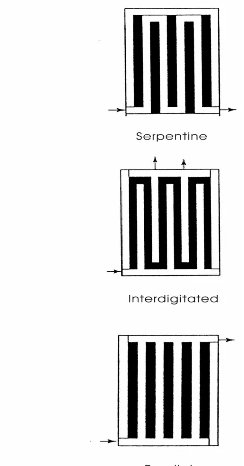
(17) contact area of catalyst and the electrolyte. Ohm’s resistance is caused by the contact resistance, electrode, membrane, proton conductivity and electron of reactant gas. The insufficient amount of reactant gas can cause the voltage drop. The voltage drop by Ohm’s resistance or insufficient amount of reactant gas is related with water balance of the interior of cells. Apparently, the three factors mentioned above are the key issues for improving the performance of fuel cells. Therefore, a good understanding of the design effects and operation conditions on the cell potential is required in order to reduce the polarization. Fig. 1-3 shows the schematic diagrams of serpentine, interdigitated, parallel flow channels. In the serpentine design, the flow snakes backward and forward, from one edge of cell to the other, in a small number of channels grouped together. It creates a long flow path for reactants in the cell. In the interdigitated design, it has inter-linked finger-like channels with dead ends. In the parallel design, it consists of a series of narrow parallel rectangular channels. This work is interesting in the design of channel, which corresponds to the mass transportation of the reacting gases and water.. Inside the fuel cell, the reactant concentration is influenced. by the mass transport between the gas channels and gas diffusion layers. Therefore, the design of the gas channels is one of the important factors to determine the fuel cell performance.. It. motivates the present study to carry out such research subject by using the numerical simulation. 5.

(18) 1.2 Literature review: Kornyshev [1] et al. investigated the gas or liquid consumption rates in the feed channels of a PEM fuel cell. Analytical expressions, which define profiles of feed concentration along the channel, and expression for characteristic length of feed consumption were computed. Nguyen [2] aimed the reactant gases (liquid) in the channel and mass and thermo transport along the channel. The conclusion. indicated. that. the. optimum. of. improving. cell. performance is increasing the saturated water temperature of inlet gases. Yi and Nguyen [3] extended the work of last reference. They showed that: (1) a higher gas flow rate through the electrode will improve the electrode performance (i.e., average current density) only when it helps to make the diffusion layer thinner; (2) The electrode average current density decreases with an increase in the shoulder width of the gas channel; (3) The electrode average current density decreases with an increase in the electrode thickness when all other dimensions and the pressure gradient are kept the same. Kumar [4] simulated the effects of channel dimensions and shape on hydrogen consumption at the anode. The results showed the optimum values for each of the dimensions (channel width, land width and channel depth) and shapes of cross-section (triangular, hemispherical and square). Yi and Nguyen [5] developed the interdigitated flow channel, which had a dead-end to force the gases through the porous electrode.. Such. design furthermore improved the mass-transport limitations in the 6.

(19) porous electrode by flooding. Nguyen [6] investigated the effect of liquid water on interdigitated flow channel.. The results indicated. that the cell performance can be improved with the adequate thickness for membrane and with increasing the number of flow channels. Kazim [7] and Chen [8] compared the PEM fuel cell performance of the serpentine and interdigitated flow channels. He found that the limiting current density with an interdigitated flow channel is about three times with the serpentine one. The results also demonstrated that the interdigitated flow channel can double the maximum power density. Yan [9] investigated the effects of the different inlet velocity and the ratio of channel width ( l channel ltotal ) on the performance. They also investigated the effects of channel number (single, two and four channels) on the cell performance. This study indicated that the single channel will cause dead-zone at the shoulder of the bio-polar plant, therefore, the cell performance increases as the number of channels increases. Bernardi [10] focused on the humidification requirements of the inlet gases in order to maintain water balance in a PEM fuel cell. Bernardi and Verbrugge [11] investigated the model of reactant gases transportation.. They used Nerst-Planck equation to. describe the proton transportation.. They also revised the effect on. potential gradient, pressure gradient and convection in porous media according to Schl ó gl’s velocity of proton transportation. 7.

(20) equation.. Further, they used Bulter-Volmer equation to describe. the value of electric current, Stefan-Maxwell equation to describe the. transportation. for. multi-component. gas. diffusion,. and. developed a one-dimensional isothermal cell model. Wang [12] applied a transient, multidimensional model, which included the source term in momentum equation to revise the transportation in porous media, and they reduced the momentum equation to Darcy equation. The two-dimension electrochemical and gases transport simulations revealed that in the presence of hydrogen dilution in the fuel stream, hydrogen is depleted at the reaction surface, resulting in substantial anode mass transport polarization and hence a lower current density that is limited by hydrogen transport from the fuel stream to the reaction site. Gurau [13] developed a one-dimensional half-cell model, which considered the presence of water and liquid water in the gas diffuser and catalyst layers, accounting by means of effective porosities that describe the porous media when the pores are partially filled with liquid at thermodynamic and hydrodynamic equilibrium. The results showed the value of the limiting current density decreases when the gas diffuser is flooded, but the excess liquid water in the catalyst layer dose not influence the value of the limiting current density. The liquid water content in the catalyst layer influences the polarization curve at values of current density is lower than the limiting current, especially at those regimes where diffusion is the rate-limiting step. Springer [14] and Rowe [15] 8.

(21) developed an isothermal one-dimensional model; they applied the water and water vapor balance in the interface between membrane and electrode, and used Stefan-Maxwell equation to describe the transportation of reactant gases. The results showed the temperature distribution within the PEM fuel cell is affected by water phase change in the electrodes, especially for a saturated reactant streams, and large peak temperature occurs within the cell at lower cell operation temperature and for partially humidified reactants as a result of increased membrane resistance arising from reduced membrane hydration. Singh, Lu and Djilali [16] developed a two-dimensional mass transport in PEM fuel cell. The results showed that the 2-D model is more conservative than 1-D process. Specially, the 2-D model results in: (1) slightly lower cell voltage; (2) severe concentration polarization taking place at much lower current density; and (3) more humidification requirements at lower current density. Hsing and Futerko [17] used the finite elements. method. to. solve. the. continuity,. potential. and. Stefan-Maxwell equations in the flow channel and gas diffusion layer. Their results inducated that the resistance of Nafion membrane in PEM fuel cell is a function of operating current density and pressure, and the fluid flow streamlines, gas mole fractions, membrane water content are shown as a function of pressure. Springer [18] investigated the electrochemical reaction and mass transport of the cathode and cathode gases diffuser. In this study, the voltage loss at the cathode side was the major loss of the cell performance. Also, they indicated the voltage loss relative small 9.

(22) when the inlet fuel was oxygen rather than the air.. In fact,. consider the cost factor; the inlet fuel is usually feed with air. They also investigated the effects of catalyst layer thickness to the cell performance. The results indicated that the cathode voltage loss decreases with catalyst layer thickness because the resistance of the catalyst layer is smaller when the catalyst layer is thinner. Both Dutta [19] and Berning [20] included the source terms by revising the chemical reaction term. They computed the velocity and mass fraction distributions of reactant gases by three-dimensional model. They showed that the significant temperature gradients exit within the cell, whereas the slight temperature differences of several degrees K exist within the MEA. Kim et al. [21] indicated that the mass transport limitation will quickly decrease the cell voltage when cell operates at high current density. Furthermore, they investigated the effects of temperature, pressure and the feed fuel to the cell performance. The predictions indicated that flow distribution and current production are affected significantly by each other Hum and Li [22] developed a two dimensional, steady state, isothermal,. fully. humidified. PEM. fuel. cell. model,. whose. electrochemical reaction was determined from Butler-Volmer equation. The results showed that the cathode catalyst layer exhibits more pronounced changes in potential, and the reaction rate and current density generation are than those of anode catalyst layer counterparts due to the lager cathode activation 10.

(23) over-potential and relatively low diffusion coefficient of oxygen. Therefore, the voltage loss in the anode catalyst layer is negligibly small due to the much fast hydrogen oxidation kinetics. Amphlett et al. [23, 24] developed a parametric model of a single PEM cell by using a mechanistic approach.. A number of. grouped parameters are identified and fitted into the empirical data measured from a Ballard Mark Ⅳ single cell.. 1.3 Scope of present study: By the literature review mentioned above, the design of interdigitated flow channels indeed has great influence on the mass transport between inlet gas channel and gas diffuser that affects the performance of PEM fuel cell. However, the mass transport of outlet gas channels is restricted by transport limitation, and the pressure drop especially near dead-end is so large that it might ruin the MEA.. In the present work, it intends to modify the parallel flow. channels by using tapering cross section area along the gases channels, which are expected to enhance the convection to improve the mass transport between the gases channels and the gas diffuser. In the present simulation work, which uses a commercial code FEMLAB as the tool, it takes a step-by-step procedure.. At. the first, the one dimensional (1-D) simulation is taken, and its predicted results are compared with the ones obtained from the analytical solution of Gurau [13]. 11. Then, the two dimensional.

(24) simulation is carried out, and its predictions are compared with those by Yan [9].. The main purpose of using 1-D and 2-D models. are to verify the importance of convection effects in the PEM fuel cell.. Finally, the 3-D model also considers the convection effects.. However, its main emphasis is the effect of flow channel design on the fuel cell performance. introduced. and. discussed. The parametric studies will be in. Chapter. Four.. Eventually,. according to the resultant effects of convection to mass transport of cell performance, this work can design the optimum tapering-ratio of gas channel outlet cross section to improve the efficiency of the mass transport and gas transport limitation between the gases channel and the gas diffuser.. 12.

(25) Fig. 1-1 The basic structure of PEM fuel cell. Fig. 1-2 The basic theory of PEM fuel cell 13.

(26) Fig. 1-3 The schematic diagrams of serpentine, interdigitated, parallel flow channels.. 14.

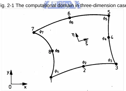
(27) Chapter 2 Mathematical Model Since the present work considers the three models, which are 1-D, 2-D and 3-D, respectively, only the 3-D model is presented for the general purpose.. 2.1 Model assumptions The model region consists three major parts: they are gas channel, gas diffusion layer and catalyst layer. Because the activation over potential of hydrogen is much lower that that of oxygen, the effect of the chemical reaction at anode can be neglected [21]. In this thesis, the effects of inlet velocity and tapering ratio of the outlet gas channel cross section to inlet one on the flow dynamics and electrochemical reaction will be investigated. The. three-dimension. computational. domain. employed. for. simulation is shown in Fig. 2-1. In order to acquire a numerically tractable solution, it is necessary to make some simplifications but without losing the main physical features. The assumptions are: 1. The flow in the channel is considered incompressible, laminar and isothermal. 2. The fuel cell operates under steady-state conditions. 3. The inlet fuel is fully saturated with water vapor. 4. All gases are assumed as ideal gases. 5. The product water is assumed to be in gas phase. 6. The diffusion coefficient is assumed to be constant. 15.

(28) 7. The over-potential is used as an operational parameter and is specified as a fixed value at each current density. 8. The catalyst layer is assumed to be a thin interface, where sink and source terms for the reactants are specified.. Therefore, it. is assumed a very thin interface without specifying its thickness.. 2.2 Governing equations The governing equations include the continuity equation, momentum conservation equations (Navier-Stokes equations) and mass conservation equation. In the 1-D model, the y- and z-direction are ignored; in the 2-D model, the z-direction is ignored. Based on the above assumptions, the 3-D model governing equations are given below.. 2.2.1.1 Gases channels Continuity equation: ρ. ∂ (u ) ∂ (v ) ∂ (w ) +ρ +ρ =0 ∂x ∂y ∂z. (2-1). The momentum conservation equations: ρu. ⎛ ∂ 2u ∂ 2u ∂ 2u ⎞ ∂u ∂u ∂u ∂p + ρv + ρw = − + µ ⎜⎜ 2 + 2 + 2 ⎟⎟ ∂x ∂y ∂z ∂x ∂y ∂z ⎠ ⎝ ∂x. (2-2). ρu. ⎛ ∂ 2v ∂ 2v ∂ 2v ⎞ ∂v ∂v ∂v ∂p + ρv + ρw = − + µ ⎜⎜ 2 + 2 + 2 ⎟⎟ ∂x ∂y ∂z ∂y ∂y ∂z ⎠ ⎝ ∂x. (2-3). ρu. ⎛ ∂2w ∂2w ∂2w ⎞ ∂w ∂w ∂w ∂p + ρv + ρw = − + µ ⎜⎜ 2 + 2 + 2 ⎟⎟ ∂x ∂y ∂z ∂z ∂y ∂z ⎠ ⎝ ∂x. (2-4). 16.

(29) The species equation for multi-species is according to the mass transport equation: ρu. ∂( yi ) ∂( yi ) ∂y ⎞ ∂( yi ) ∂y ⎞ ∂y ⎞ ∂ ⎛ ∂ ⎛ ∂ ⎛ + ρv + ρw = ρ ⎜ Di , j i ⎟ + ρ ⎜⎜ Di , j i ⎟⎟ + ρ ⎜ Di , j i ⎟ ∂x ∂y ∂z ⎝ ∂z ⎠ ∂z ∂x ⎝ ∂x ⎠ ∂y ⎝ ∂y ⎠. (2-5) where i represents oxygen, nitrogen and water vapor, respectively, and Di , j is the diffusivity of the species. For the binary diffusivities, Di , j , it should be derived from the Stefan-Maxwell equation, which has a very complicated formulation. In this thesis, it adopts the experimental value according to [10], which is obtained at atmospheric pressure p 0 and taken and scaled with the temperature and pressure: ⎛ p ⎞⎛ T ⎞ Dij = Dij (T0 , p 0 )⎜⎜ ⎟⎟⎜⎜ ⎟⎟ ⎝ p 0 ⎠⎝ T0 ⎠. 1 .5. (2-6). The average molecular mass of gas mixture is calculated by: M =. 1 yO2 M O2. +. y H 2O M H 2O. +. 1 − y o2 − y H 2 O M N2. (2-6) The mass fraction of the saturated water vapor is related to the molar fraction by: y H 2O =. p Hsat2O M H 2O p. (2-7). M. where the water saturated pressure is calculated from the following expression [18]: log10 p Hsat2O = −2.1794 + 0.2953T − 9.1837 × 10 −5 T 2 + 1.4454 × 10 −7 T 3. (2-8) 17.

(30) Boundary conditions of gas channel: At the inlet of gas channel: u = u 0 ( specified ), v = w = 0 y O2 = 0.17, y H 2O = 0.12, y N 2 = 0.71. (2-9) At the walls of the gas channel, the boundary conditions are no-slip conditions u=v=w=0 ∂yi =0 ∂z. (2-10). At the outlet of the gas channel, the boundary conditions are: ∂p ∂x. =0 outlet. ∂yi =0 ∂x. (2-11). At the interface between the gas channel and Gas Diffusion Layers, the boundary conditions for mass fraction are: ∂y i τ = ε 1 Di , j ∂x ∂y i τ = ε 1 Di , j ∂y. ∂y i ∂x ∂y i ∂y. (2-12) (2-13). ∂y ∂y i τ = ε 1 Di , j i ∂z ∂z. (2-14). 2.2.2 Gas Diffusion Layers (GDL) The gas diffusion layers are made of graphite cloth and formed as porous media.. The momentum equation has a source term for. the porous media, used for flow through diffusion layer, which is described by Darcy’s law [19]. Continuity equation: ρ. ∂ (u ) ∂ (v ) ∂ (w ) +ρ +ρ =0 ∂x ∂y ∂z. (2-15). 18.

(31) Momentum conservation equations: 2τ 2 ⎛ ∂u ∂ 2u ∂ 2u ⎞ ε 1 µ ∂u ⎞ ∂u τ ∂p τ ⎛∂ u ⎟ ⎜ ⎜ ⎟ w − u v ε 1 ⎜ ρu + ρ +ρ ⎟ = −ε 1 ∂x + ε 1 µ ⎜ ∂x 2 + ∂y 2 + ∂z 2 ⎟ z y k x ∂ ∂ ∂ ⎝ ⎠ p ⎠ ⎝. τ. (2-16) 2τ 2 ⎛ ∂v ∂ 2v ∂ 2v ⎞ ε1 µ ∂v ⎞ ∂v τ ∂p τ ⎛∂ v ⎟ ⎜ ⎜ ⎟ w − v v ε 1 ⎜ ρu + ρ +ρ ⎟ = −ε 1 ∂y + ε 1 µ ⎜ ∂x 2 + ∂y 2 + ∂z 2 ⎟ z y k x ∂ ∂ ∂ ⎝ ⎠ p ⎠ ⎝. τ. (2-17) 2τ 2 ⎛ ∂w ∂ 2 w ∂ 2 w ⎞ ε1 µ ∂w ⎞ ∂w τ ∂p τ ⎛∂ w ⎟ ⎜ ⎜ ⎟ w − w v ε 1 ⎜ ρu +ρ +ρ ⎟ = −ε 1 ∂z + ε 1 µ ⎜ ∂x 2 + ∂y 2 + ∂z 2 ⎟ z y k x ∂ ∂ ∂ ⎝ ⎠ p ⎠ ⎝. τ. (2-18) where the ε and τ are the porosity and tortuosity of the gas diffusion layer, respectively, and they are assumed to be constant, and k p denotes the hydraulic permeability. The species equation is: ⎡. ε 1τ ⎢ ρu ⎣. ∂y ⎞ ∂y ⎞⎤ ∂y ⎞ ∂( y i ) ∂( y i ) ∂( y i )⎤ ∂ ⎛ ∂ ⎛ ∂ ⎛ τ ⎡ + ρv + ρw = ε 1 ⎢ ρ ⎜ Di , j i ⎟ + ρ ⎜⎜ Di , j i ⎟⎟ + ρ ⎜ Di , j i ⎟⎥ ⎥ ∂y ⎝ ∂y ⎠ ∂z ⎝ ∂z ⎠⎦ ∂x ⎠ ∂x ∂y ∂z ⎦ ⎣ ∂x ⎝. (2-19). Boundary conditions: No-slip conditions are applied at the GDL walls. u = v = w = 0 and. ∂y i ∂y i = =0 ∂x ∂y. (2-20). Interface conditions between gas diffusion layer and catalyst layer: At the interface between the GDL and catalyst layer, the boundary conditions are: −. kp. µ. ∇p = V −. +. and. ∂yi =0 ∂z. (2-21). As mentioned before, the catalyst layer is treated as a thin interface and adhesive on the boundary wall of the gas diffusion 19.

(32) layer, where sink and source terms for the reactants are implemented. Due to the treatment of infinitesimal thickness, the source terms are actually implemented in the last grid cell of the gas diffusion layer. At the interface between the GDL and catalyst layer, the boundary conditions for mass fraction are: ∂yi + uyi ) = S k ∂x ∂y ε 1τ ( Di , j i + vy i ) = S k ∂y. ε 1τ ( Di , j. ε 1τ ( Di , j. (2-22) (2-23). ∂y i + wy i ) = S k ∂z. (2-24). When S k is the source term for oxygen at the cathode side, it is described by [19] as S O2 = −. jc 4 F ⋅ cOref2. (2-25). For water, it is given by: S H 2O =. jc 2 F ⋅ cOref2. where. jc. (2-26) is the local current density, described by the. Bulter-Volmer equation: ⎛ cO j c = j 0ref ⎜ ref2 ⎜ cO ⎝ 2. ⎞⎡ ⎛ α a F ⎞ ⎛ α F ⎞⎤ ⎟ ⎢exp⎜ η ⎟ − exp⎜ − c η ⎟⎥ ⎟ ⎣ ⎝ RT ⎠ ⎝ RT ⎠⎦ ⎠. (2-27). in which c denotes the concentration of the reactants and α is the transfer coefficient. The over-potential η can be measured a priori. The range of the over-potential depends on the loading of the catalyst and exchange current density ( j 0ref ), which is related with. 20.

(33) operating temperature. The local current density generated at the reaction interface is calculated by the Tafel equation [13]: i = nFDij. ∂y O2 ∂z. (2-28) z=H. where n is the number of electron transferred during the ORR (oxygen reduction reaction) and H is the total height of the Gas channel and GDL. The average current density on the ORR reaction interface is determined as: iavg =. W L 1 i( x, y )dxdy ∫ W × L 0 ∫0. (2-29) where W and L are the total width and length of the model scale.. 2.3 Nondimensionalization of the governing equations In this thesis, the model is solved nondimensionally. Therefore, a nondimensional procedure is carried out throughout the model.. The following dimensionless variables and parameters. are introduced in advance: U=. P=. u v w x y z , V = , W = , X = , Y = , Z = u0 u0 u0 De De De. p − pi. ρU i. 2. ,. Re =. ρU i D e µ. ,. kp =. kp De. 2. ,. Sc =. µ ρD. (2-30). The resultant nondimensional governing system is described as follows.. 21.

(34) 2.3.1 The gas channel Continuity equation: ∂U ∂V ∂W =0 + + ∂X ∂Y ∂Z. (2-31). Navier-Stokes equations: U. 1 ∂ 2U ∂ 2U ∂ 2U ∂P ∂U ∂U ∂U ( ) + + + =− +W +V ∂X Re ∂X 2 ∂Y 2 ∂Z 2 ∂Z ∂Y ∂X. (2-32). U. ∂V ∂V ∂V ∂P 1 ∂ 2V ∂ 2V ∂ 2V ( ) +V +W =− + + + ∂X ∂Y ∂Z ∂Y Re ∂X 2 ∂Y 2 ∂Z 2. (2-33). U. ∂W ∂W ∂W ∂P 1 ∂ 2W ∂ 2W ∂ 2W ( ) +V +W =− + + + ∂X ∂Y ∂Z ∂Z Re ∂X 2 ∂Y 2 ∂Z 2. (2-34). Mass transport equation: ∂y ⎞ 1 ⎛ ∂ 2 y i ∂ 2 y i ∂ 2 yi ∂y ⎛ ∂y ⎜ + + S c ⎜U i + V i + W i ⎟ = ∂Z ⎠ Re ⎜⎝ ∂X 2 ∂Y 2 ∂Z 2 ∂Y ⎝ ∂X. ⎞ ⎟⎟ ⎠. (2-35). Boundary conditions: At the inlet of the gas channel: U = 1 and V = W = 0 y O2 = 0.17, y H 2O = 0.12, y N 2 = 0.71. (2-36) At the walls of the gas channel and gas diffusion layer: U = V = W = 0 and. ∂y i ∂yi =0 = ∂Y ∂Z. (2-37). At the outlet of the gas channel: ∂P = 0 and ∂X. ∂yi =0 ∂X. (2-38). At the interface between the gas channel : τ. ∂y i ∂y i ε = 1 ∂X Re S c ∂X. (2-39). τ. ∂y i ∂y i ε = 1 ∂Y Re S c ∂Y. (2-40) 22.

(35) τ. ∂y i ∂y i ε = 1 ∂Z Re S c ∂Z. (2-41). 2.3.2 Gas diffusion layers Continuity equation: ∂U ∂V ∂W + + =0 ∂X ∂Y ∂Z. (2-42). Navier-Stokes equations: ∂ 2U ∂ 2U ∂ 2U ∂P 1 ⎛ ∂U 1 1 ∂U ⎞ ∂U + + U ( 2 + )− U +W +V ⎟=− τ ⎜ τ 2 2 ∂X Re ε 1 ∂X ∂Z ⎠ ∂Y ε 1 ⎝ ∂X ∂Y ∂Z kp. (2-43). 1 1 ⎛ ∂V 1 ∂ 2V ∂ 2V ∂ 2V ∂P ∂V ⎞ ∂V W V U ( )− V + + + = − + + ⎟ τ ⎜ τ 2 2 2 ∂Y Re ε 1 ∂X ∂Z ⎠ ∂Y ε 1 ⎝ ∂X ∂Z ∂Y kp. (2-44). ∂ 2W ∂ 2W ∂ 2W ∂P 1 ⎛ ∂W 1 1 ∂W ⎞ ∂W + + U ( 2 + ) − W (2-45) +W +V ⎟=− τ ⎜ τ 2 2 ∂Z Re ε 1 ∂X ∂Z ⎠ ∂Y ∂Y ∂Z ε 1 ⎝ ∂X kp. Mass transport equation: ∂y i ⎞ 1 ⎛ ∂ 2 y i ∂ 2 y i ∂ 2 yi ∂y i ⎛ ∂y i ⎜ W V + + S c ⎜U + + ⎟= ∂Z ⎠ Re ⎜⎝ ∂X 2 ∂Y 2 ∂Z 2 ∂Y ⎝ ∂X. ⎞ ⎟⎟ ⎠. (2-46). Boundary conditions: At the interface between the GDL and catalyst layer: − k p ⋅ ∇P = V and. ∂yi =0 ∂Z. (2-47). At the GDL walls: U =V =W = 0. and. ∂y i ∂yi =0 = ∂X ∂Y. (2-48). At the interface between the GDL and catalyst layer, the boundary conditions of mass fraction are: 23.

(36) ε 1τ (. ∂y i + U ⋅ yi ) = S k ∂X. (2-49). ε 1τ (. ∂y i + V ⋅ yi ) = S k ∂Y. (2-50). ε 1τ (. ∂yi + W ⋅ yi ) = S k ∂Z. (2-51). where S k is the dimensionless source term. For oxygen: Sk = −. ρDe 1 jc 4 F µCtotal. (2-52). and for water: Sk =. ρDe 1 jc 2 F µCtotal. (2-53). 2.4 Normalization The concept of subdividing a physical domain into elements is adopted for problem of describing a variation in the variable across the whole domain such that it becomes far simpler since the variation can now be related within each element.. Therefore, it. has to change the globe coordinates into the local one.. This. procedure is termed as normalization. According to the Galerkin Weighted Residuals Approach, the Navier-Stokes equations can become. ∫ ∫. Ωe. Ωe. ⎡ ⎛ ∂U ∂U ∂U ⎞ ∂P N i ⎛ ∂ 2U ∂ 2U ∂ 2U ⎞⎤ ⎜⎜ 2 + ⎟ dΩ = 0 N U V W + + N + − + ⎟ ⎢ i⎜ i 2 2 ⎟⎥ X Y Z X Re ∂ ∂ ∂ ∂ X Y Z ∂ ∂ ∂ ⎝ ⎠ ⎝ ⎠⎦ ⎣. (2-54). ⎡ ⎛ ∂V ∂V ∂V ⎞ ∂P N i ⎛ ∂ 2V ∂ 2V ∂ 2V ⎞⎤ ⎜ ⎟⎥ dΩ = 0 +V +W − + + ⎟ + Ni ⎢ N i ⎜U ∂Y ∂Z ⎠ ∂Y Re ⎜⎝ ∂X 2 ∂Y 2 ∂Z 2 ⎟⎠⎦ ⎣ ⎝ ∂X. (2-55). 24.

(37) ∫. ⎡ ⎛ ∂W ∂W ∂W ⎞ ∂P N i ⎛ ∂ 2W ∂ 2W ∂ 2W ⎞⎤ ⎜ ⎟⎥ dΩ = 0 +V +W − + + ⎟ + Ni ⎢ N i ⎜U ∂Y ∂Z ⎠ ∂Z Re ⎜⎝ ∂X 2 ∂Y 2 ∂Z 2 ⎟⎠⎦ ⎣ ⎝ ∂X. Ωe. (2-56). By Reducing the second order terms and pressure terms through Gauss integration formula, it gives. ∫. ∂N i ∂P dΩ = ∫ P N i n x d Γ − ∫ P dΩ Γ Ω ∂X ∂X ∂N i ∂P dΩ Ni dΩ = ∫ P N i n y dΓ − ∫ P Γe Ωe ∂Y ∂Y. ∫. Ni. ∫. (2-57a). Ni. Ωe. e. Ωe. ΩE. e. (2-57b). ∂N i ∂U ∂U ∂ 2U dΩ dΩ = ∫ N i dΓ − ∫ 2 Γ Ω ∂X ∂ X ∂X ∂X e. (2-57c). e. ∂N i ∂U ∂ 2U ∂U ∫Ω ∂Y 2 dΩ = ∫Γ N i ∂Y dΓ − ∫Ω ∂Y ∂Y dΩ ∂N i ∂U ∂U ∂ 2U N ∫Ω i ∂Z 2 dΩ = ∫Γ N i ∂Z dΓ − ∫Ω ∂Z ∂Z dΩ ∂N i ∂V ∂ 2V ∂V N ∫ΩE i ∂X 2 dΩ = ∫Γe N i ∂X dΓ − ∫Ωe ∂X ∂X dΩ ∂N i ∂V ∂ 2V ∂V N ∫ΩE i ∂Y 2 dΩ = ∫Γe N i ∂Y dΓ − ∫Ωe ∂Y ∂Y dΩ ∂N i ∂V ∂V ∂ 2V N ∫Ω E i ∂Z 2 dΩ = ∫Γe N i ∂Z dΓ − ∫Ωe ∂Z ∂Z dΩ ∂N i ∂W ∂W ∂ 2W N ∫Ω E i ∂X 2 dΩ = ∫Γe N i ∂X dΓ − ∫Ωe ∂X ∂X dΩ ∂N i ∂W ∂W ∂ 2W N ∫Ω E i ∂Y 2 dΩ = ∫Γe N i ∂Y dΓ − ∫Ωe ∂Y ∂Y dΩ ∂N i ∂W ∂ 2W ∂W N ∫ΩE i ∂Z 2 dΩ = ∫Γe N i ∂Z dΓ − ∫Ωe ∂Z ∂Z dΩ. (2-57d). Ni. E. E. e. e. e. (2-57e). e. (2-57f) (2-57g) (2-57h) (2-57i) (2-57j) (2-57k). By including Eq. 2-54~2-56 into above equations, they become:. ∫. Ωe. =. ∫. ⎡ ⎛ ∂U ∂Ni 1 ⎛ ∂Ni ∂U ∂Ni ∂U ∂Ni ∂U ⎞⎤ ∂U ∂U ⎞ +V +W + ⎜ + + ⎟ dΩ ⎟−P ⎢Ni ⎜U ∂Y ∂Z ⎠ ∂X Re ⎝ ∂X ∂X ∂Y ∂Y ∂Z ∂Z ⎠⎥⎦ ⎣ ⎝ ∂X. ∂U 1 dΓ − ∫ P Ni nx dΓ Ni ∫ Γe Re Γe ∂n. Ωe. (2-58a). ⎡ ⎛ ∂V ∂Ni 1 ⎛ ∂Ni ∂V ∂Ni ∂V ∂Ni ∂V ⎞⎤ ∂V ∂V ⎞ +V +W ⎟ − P + ⎜ + + ⎟⎥ dΩ ⎢Ni ⎜U ∂Y ∂Z ⎠ ∂Y Re ⎝ ∂X ∂X ∂Y ∂Y ∂Z ∂Z ⎠⎦ ⎣ ⎝ ∂X. 25.

(38) =. ∫. 1 ∂V Ni dΓ − ∫ P Ni n y dΓ ∫ Γ Γe Re e ∂n. Ωe. =. (2-58b). ⎡ ⎛ ∂W ∂Ni 1 ⎛ ∂Ni ∂W ∂Ni ∂W ∂Ni ∂W ⎞⎤ ∂W ∂W ⎞ +V +W + ⎜ + + ⎟ dΩ ⎟−P ⎢Ni ⎜U ∂Y ∂Z ⎠ ∂Z Re ⎝ ∂X ∂X ∂Y ∂Y ∂Z ∂Z ⎠⎥⎦ ⎣ ⎝ ∂X. 1 ∂W Ni dΓ − ∫ P Ni nz dΓ ∫ Γe Re Γe ∂n. (2-58c). Through normalization, the governing equations can be expressed by matrix form: U (e ) = [N ] {U }. (2-59a). V (e ) = [N ] {V }. (2-59b). W (e ) = [N ] {W }. (2-59c). (e ). (e ). (e ). [N ]1×8 = [N1 , N 2 , {U }( ) e. 8×1. . . . , N8 ]. (2-60). ⎧U1 ⎫ ⎪⎪ U ⎪⎪ = ⎨ 2⎬ ⎪M ⎪ ⎩⎪ U 8 ⎭⎪. (2-61a). ⎧ V1 ⎫ ⎪V ⎪ {V}8(e×1) = ⎪⎨ 2 ⎪⎬ ⎪M ⎪ ⎪⎩V8 ⎪⎭. {W }8(e×)1. (2-61b). ⎧W1 ⎫ ⎪⎪W ⎪⎪ = ⎨ 2⎬ ⎪ M⎪ ⎪⎩W8 ⎪⎭. (2-61c). where the shape functions are given by, N1 =. -1 (1−ξ 4. )( 1 − η )(1 + ξ + η ). N2 =. 1 (1 − ξ 2 2. N3 =. 1 (1+ ξ 4. )( 1 − η )(ξ − η − 1). (2-62c). N4 =. 1 (1+ ξ 2. ) (1 −η 2. (2-62d). (2-62a). )( 1 −η ). (2-62b). ) 26.

(39) N5 =. 1 (1+ ξ 4. )( 1 + η )(ξ + η − 1). N6 =. 1 (1 − ξ 2 2. )( 1 + η ). (2-62f). N7 =. −1 (1−ξ 4. )( 1 + η )(1 + ξ − η ). (2-62g). N8 =. 1 (1−ξ 2. ) (1 −η 2. (2-62e). ). (2-62h). Fig. 2-2 shows the parabolic eight node element, which possesses the typical node numbering for associated discrete variables. The single element can be expressed as matrix form,. ( [C ]( ) + [K ]( ) + λ [L]( ) ){q}( ) = { f }( ) e. e. e. e. e. (2-63). where {q}(e ) = [U1 , U 2 , . . . , U 8 , V1 , V2 , . . . , V8 , θ1 , θ 2 , . . . , θ 8 ]t. [C ](e ) : The matrix of the non-linear intera of velocity [K ](e ) : The matrix of shape functions and time terms [L ](e ) : The matrix of penalty function { f }(e ) : The matrix of the given vectors of right hand side The matrix of the single element is,. ( [C ] + [K ] + λ [L] ){q} = { f }. (2-64). The criterion of convergence is,. (. MAX {q}. m +1. − {q}. m. ) {q}. m +1. < 10 −3. (2-65). 27.

(40) Fig. 2-1 The computational domain in three-dimension case. Fig. 2-2 The configuration of parabolic eight node element. 28.

(41) CHAPTER 3 A Brief Introduction of FEMLAB 3.1 Briefing FEMLAB is an interactive environment foe modeling and simulating scientific and engineering problems based on partial differential equations (PDEs), which are the fundamental basis of the laws of science. FEMLAB’s multi-physics feature is allowed to simultaneously model any combination of phenomena. The ability to define multi-physics problems is supported by numerical machinery that guides the solver to the correct solution, even for highly nonlinear problems.. The. current. available. modules. with. associated. application areas are: (1) The Chemical Engineering Module: This module includes transport phenomena and chemical reaction in reactors and operations. (2) The Electro-magnetic Module: This module includes wave propagation and mode analysis in microwave engineer and photonics. (2) The Structural Mechanics Module: This module includes static, dynamic, and eigenfrequency structural analysis. The Chemical Engineering Module provides tailored interfaces and formulations for problems involving momentum, mass and heat transport coupled with chemical reactions. Characterizing the flow 29.

(42) with Navier-Stokes equations in chemical module, the chemical reactions are easily represented by source or sink terms in the mass and heat balances and can be of any arbitrary order. All formulations exit for both Cartesian coordinates and axisymmetry and for stationary and time dependent cases.. 3.2 The Finite Element Method The mesh is a partition of the geometry into small units of a simple shape. In 1-D the method partitions the subdomains into small intervals or mesh elements. The endpoints of the mesh intervals are called mesh vertices. In 2-D, the method partitions the subdomains into triangles, or mesh elements. The sides of the triangles are called mesh edges, and their corners are mesh vertices. A mesh edge must not contain mesh vertices in its interior. Similarly, the boundaries defined in the geometry are partitioned into mesh edge (so-called boundary elements) that must conform with the triangles if there is an adjacent subdomain. There might also be isolated points in the geometry. These also become mesh vertices. Similarly, in 3-D the method partitions subdomains into tetrahedrons, whose faces, edges and corners are called mesh faces, mesh edges, and mesh vertices. It partitions boundaries in the geometry into triangular boundary elements (mesh faces); it partitions geometry edges into mesh edges; and isolated geometry vertices become mesh vertices (sometimes called node points). Since we have a mesh, we can introduce approximations to the 30.

(43) dependents variables. The idea is to approximate u (assumed single variable) with a function that we can describe with a finite number of parameters, the so-called degrees of freedom (DOF). Inserting this approximation into the weak form of the equation generates a system of equations for the degrees of freedom. Assume that a mesh consists of just two mesh interval: 0 < x < 1 and 1 < x < 2 . Linear elements mean that on each mesh interval the continuous functions u is linear. Set x1 = 0 , x2 = 1 , and x3 = 2 . Denote these as U 1 = u (0) , U 2 = u (1) , U 31 = u (2) , these are the degrees of freedom. Now we can express u (x) as: u ( x) = U 1ϕ1 ( x) + U 2ϕ 2 ( x) + U 3ϕ 3 ( x). (3-1). where ϕ i (x) are certain piecewise linear functions. Namely, ϕ i (x) is the function that is linear on each mesh interval, equal 1 at the i th node point, and equal 0 at the other node points. For example:. ⎧1 − x ⎩0. ϕ1 ( x) = ⎨. if if. 0 ≤ x ≤1 1≤ x ≤ 2. (3-2). The ϕ i (x) are called the basis functions. The set of functions u (x) is a linear function space called the finite element space.. For batter accuracy, consider another finite element space corresponding to quadratic elements. Functions u in this space are 2nd-order polynomials on each mesh interval. To characterize such a function, introduce new node points at the midpoint of each mesh interval: x4 = 0.5 , x5 = 1.5 . The 2nd-order degree polynomial 31.

(44) u (x) is determined by the degree of freedom at the endpoints and. the midpoints. The u (x) is expressed as: u ( x) = U 1ϕ1 ( x) + U 2ϕ 2 ( x) + U 3ϕ 3 ( x) + +U 4ϕ 4 ( x) + U 5ϕ 5 ( x). (3-3). where the basis functions ϕ i (x) now have a different meaning. ϕ i (x) is the function that quadratic on each mesh interval, equal 1. at i th node point, and equal 0 at the other node points. For example: ⎧(1 − x )(1 − 2 x ) ⎩0. ϕ1 ( x ) = ⎨. if if. 0 ≤ x ≤1 1≤ x ≤ 2. (3-4). In general, we specify a finite element space by giving a set of basis functions. The description of the basis functions is simplified by the introduction of local coordinates. Consider a mesh elements dimension d. in a n − dimensional geometry (whose space. coordinates are denoted x1 ,..., x n ). Consider also the stander d-dimensional simplex. ζ 1 ≥ 0, ζ 2 ≥ 0,..., ζ 1 + ... + ζ d ≤ 1. (3-5). which resides in the local coordinated space parametrized by the local coordinates ζ 1 ,..., ζ d . If d =1, then this simplex is the unite interval. If d =2, it is a triangle with 45 degree angles, and if d =3 it is a tetrahedron. Now we can consider the mesh element as a linear transformation of the stander simplex. Namely, by letting global space coordinates xi be suitable linear functions of the local coordinates, we can get the mesh element as the image of the 32.

(45) stander simplex. When described in terms of local coordinates, the basis functions assume one of a few basis shapes. These are the shape functions. In the example with elements in 1-D, any basis function on any mesh elements is one of the following are: φ = ζ1 ,. φ = 1−ζ1 ,. φ =0. (3-6). Thus the first two are shape functions in the example (0 is not counted as a shape function). In the example with quadratic elements in 1-D, the shape functions are: φ = (1 − ζ 1 )(1 − 2ζ 1 ) ,. φ = 4ζ 1 (1 − ζ 1 ) ,. φ = ζ 1 (2ζ 1 − 1). (3-7). For the Lagrange element, the preceding examples are special case of the Lagrange element. Consider a positive integer k , the order of the Lagrange element. The function u in this finite element mesh are piecewise polynomials of degree k , that is, on each mesh element u is a polynomials of degree k . To describe such a function it suffices to give this value in the Lagrange points of order k . These are points whose local coordinates are integer multiples of 1 k . For example, in 2-D with k = 2 , this means that we have node points at the corners and side midpoints of all mesh triangles. For each of these node points p i , there are exits a degree of freedom U i = u ( pi ) and a basis function ϕ i . The restriction of the basis function ϕ i to mesh element is a polynomial of degree k in the local coordinates such that ϕ i = 1 at node i ,. 33.

(46) and ϕ i = 0 at the other nodes. Thus the basis functions are continuous and we have: u = ∑ U iϕ i. (3-8). i. The Lagrange element of order 1 is called the linear element. The Lagrange element of order 2 is called the quadratic elements.. 3.3 Computational Procedure The present work adopts Chemical Engineering Module in FEMLAB to simulate the channel flow in a PEMFC.. The Module. modeling procedure involves the following steps. (1) Create or import the geometry in 1D, 2D or 3D: In the draw mode, it is used to draw the geometry of the model. (2) Select the equations to define the system: The Model Navigator is multipurpose dialogs box, in which controls the general setting of a FEMLAB’s session. Multi-physics page allows to select application modes, dimension and other setting for multi-physics model. Model Navigator also shows the dependent variables, types of element and types of solver. (3) Specify the physical properties in the selected equations: The physical properties can be entered as constants in the Add/Edit Constants dialog box of the Options menu. The values used are all in SI units.. 34.

(47) (4) Set the boundary and initial conditions: Set the boundary conditions through choosing Boundary Setting from the Boundary menu. The dialog box has different options in different application modes. The coefficients in the governing equations can be interpreted, depending on the application mode from the Subdomain Setting of Subdomain menu. Initial values are also set in the Subdomain Setting dialog box. (5) Generate and refine the finite element meshes: Because FEMLAB is based on the finite element method (FEM), it needs a subdivision of the geometry, known as a mesh. A standard mesh is created automatically as entering the mesh mode. In the Mesh Parameters dialog box, it can change a different resolution or require the mesh to be denser in some parts of the geometry than in others. (6) Execute the simulation: There are two types of solvers; the direct solver and the iterative solver. The direct solver solves the linear system by Gaussian elimination. This is stable and reliable process and is well–suited for ill-conditioned system. It requires less tuning and is often faster than the iterative solvers in 1D and 2D. The elimination process sometimes needs large resources of memory and computing. times.. The. iterative. solver. generally. uses. substantially less memory than the direct one, and it is often faster in 3D. The iterative solver needs a careful selection of preconditioner for optimal performance. FEMLAB has three 35.

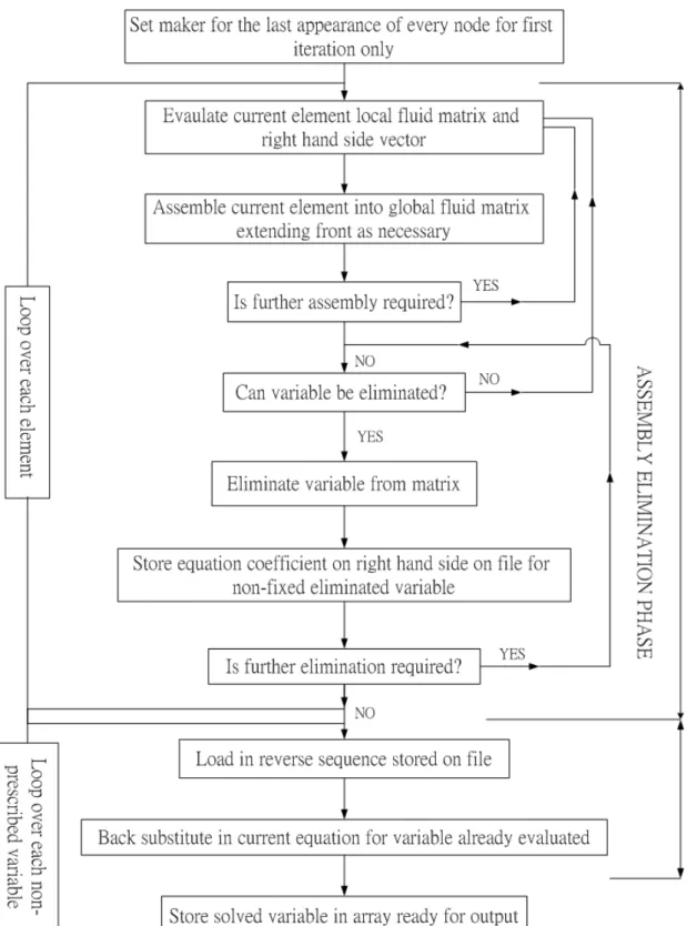
(48) iterative solvers. The Good Broyden iterative solver works well for most elliptic problems, such as the Possion, Helmholtz, and Navier-Stokes equations. The GMRES iterative solver is recommended for the Navier-Stokes equations and other non-elliptic PDE’s. The third solver is transpose-free QMR. The default preconditioner is incomplete LU factorization. This is the most general preconditioner, and it works well also for difficult problems, but it requires a careful choice of drop tolerance. The incomplete LU factorization is the preferred preconditioner for the structural mechanics and the incompressible Navier-Stokes 3-D application mode. The default drop tolerance is 10-2, which is the condition of convergence. As the drop tolerance approaches 0, the incomplete LU factorization will become more and more similar to that of using a complete LU factorization, which is equivalent to using the direct solver. The mesh quality is important for the iterative solver. By increasing the mesh quality, the iterative solver will use less iteration. (7) Visualize the results: In post mode, it can add additional types and set parameters for the different plots. The post processing utilities can visualize any valid MATLAB expression, containing, e.g., the solution variables, their derivatives and the space coordinates. Fig. 3-1 Shows the numerical computation flow chart.. 36.

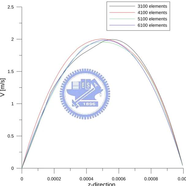
(49) 3.4 Grid tests In order to reduce the effects of mesh (elements) size and number on the accuracy of the final results, it is important to test the gird accuracy before simulation. There are three factors, which the grid tests need to take into consideration. They are the accuracy, the stable numerical process and the time, which is used to solve. In general, the more meshes (elements) the results are more accuracy, nevertheless, it costs more time. The primary sources of error associated with the application of the finite element method are: (1). Numerical round-off resulting from the necessary numerical manipulations within a computer.. (2). The tolerance set for the termination of the iterative type solution.. (3). The discretization errors arising from the finite elements approximation.. A tolerance limitation, (ϕ new − ϕ old ) ϕ new ≤ 0.1 , has been set in the model, which ϕ new is updated value of a variable (u, v, w) or yi , and ϕ old is the weighted initial value used as the iteration to evaluate ϕ new . In order to avoid the domination of round error, this check is omitted when ϕ new ≤ 10 −4 . The actual magnitude of the convergence criterion can be changed to suit a particular problem. The discretization error accrues according to three main 37.

(50) factors; the order of the interpolation functions; the size of the meshes (elements); the shape or arrangement of the elements. Fig. 3-2 shows the resultant velocity profiles at the middle of the gas channel(x-direction) with different applications of meshes under the same inlet velocity condition.. The grid tests apply four. different number elements; they are 3100, 4100, 5100 and 6100, respectively. The results show that discrepancies among the velocity profiles of 4100, 5100 and 6100 number elements are not appreciated.. Consider the trade-off between solution accuracy. and computational time, this study computes the model with 5100 number element.. 38.

(51) Fig. 3-1 The numerical computation flow chart. 39.

(52) 3100 elements 4100 elements 5100 elements 6100 elements. 2.5. 2. V [m/s]. 1.5. 1. 0.5. 0 0. 0.0002. 0.0004. 0.0006. 0.0008. 0.001. z-direction. Fig. 3-2 Grid test with the velocity profile at the middle of the gas channel(x-direction) with the same inlet velocity condition. 40.

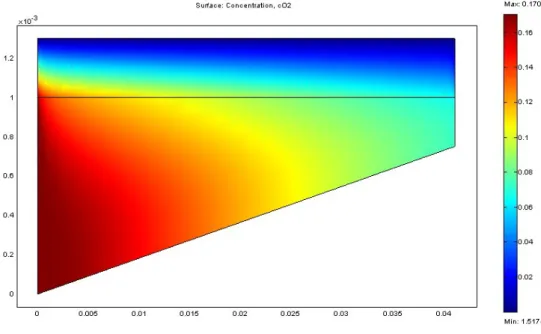
(53) Chapter 4 Results and Discussion 4.1 One-dimensional model This simulation.. thesis. starts. with. the. one-dimensional. numerical. Fig. 4-1 shows the schematic configuration of the 1-D. model. The parameters for this case are presented in Table. 4-1. In such simulation, the convention effect cannot be considered and the mass transport is only dependent on diffusion. The inlet conditions are specified as follows.. The mass concentration of. oxygen is fixed at 0.17, water is 0.12 and nitrogen is 0.71. The temperature is specified at 60°C, and the diffusion coefficients of oxygen, water and nitrogen are the same constants. The over-potential (η) is equal to 0.3. The oxidization of hydrogen is so fast that it results in a very low activation over-potential, almost equal to zero. The reduction of oxygen has the more complicated steps, causing its activation over-potential to be quite larger than the former one. Therefore, the activation over-potential of total reaction can almost regarded as the oxygen reduction in the cathode side. In this study, it uses the activation over-potential as the input parameter in the model. Diffusion describes the movement of a given species relative to the motion of the other species in a mixture. The important modes of diffusion are ordinary, Knudsen, configurationally and surface diffusion. Ordinary diffusion almost always occurs in most diffusion 41.

(54) modes; Knudsen diffusion is important only when the pore is small; configurationally diffusion takes place when the characteristic pore size is on the molecular scale; and surface diffusion involves the movement of adsorbates on surface. In a typical fuel cell model, the pores are so large that configurationally diffusion dose not occur. Surface diffusion may play an important role in interfacial reaction, but it is not considered in this study. According to the Tafel equation (Eq. 2-28), the relationship between current density and oxygen concentration is determined by given over-potential, therefore, oxygen concentration affects the cell performance directly. Fig. 4-2 shows the predicted oxygen distribution across the cell, and it compares with the analytical solution obtained by Gurau [13], which uses three different porosities (0.7, 0.5 and 0.4, respectively) in GDL. With the same applied conditions, including the application of three different porosities in GDL, the predicted oxygen concentration profile is almost identical with the one of Gurau [13].. On the other hand,. with the single value of porosity, 0.3, in GDL, the present study predicts a lower oxygen concentration over there since the lower porosity allows less oxygen to pass over GDL. The oxygen concentration decreases linearly in the gas channel and gas diffusion layer, respectively.. Nevertheless, at the interface. between two layers, the oxygen reduction level is much faster in gas diffusion layer because it is made of porous media. The diffusion layer used in the fuel cells is to maximize the interfacial area of the catalyst layer per unit geometric area. Thus, it 42.

(55) must be designed to maximize the available catalytic area while minimizing the resistances to mass transport in the electrolytic and gas phases and the electronic resistance in the solid phase. Fig. 4-3 shows the water vapor distribution across the cell. The water vapor increases linearly in the gas channel and gas diffusion layer because its production rate is stoichematically proportional to consumption rate of oxygen. The maximal concentration of water vapor occurs at the catalyst layer, and it diffuses backward from catalyst layer to the gas channel. Fig. 4-4 shows the typical fuel cell polarization curve. The curve includes a sharp drop in potential at low current density due to the sluggish kinetics of oxygen reduction reaction (ORR). This parts of the polarization curve is commonly called kinetic regime. At larger current density, it enters an ohmic regime, where the cell potential varies nearly linear with current density. At large current density, the mass transport resistance dominates and the cell potential declines rapidly as one of the reactant concentrations approaches zero at the corresponding catalyst layer. This defines the limitation of mass transport. Fig. 4-5 shows the comparison of the cell polarization curves in present 1-D model ( ε = 0.3, 0.4 and 0.5, respectively) and Gurau [13] ( ε = 0.3, 0.4 and 0.5, respectively) with a reversible cell voltage ( Voc =0.9). In general, the polarization curve decreases quickly at the high current density, since the cell is operated under limiting of mass transport so that there is not enough oxygen for chemical 43.

(56) reaction. The polarization curve obtained from the present study is exactly the same as the one by Gurau [13].. 4.2 Two-dimensional model In 2-D model, we consider the effects of convection along the gas channel with the tapering cross section to the outlet gas channel to enhance the gas to enter the gas diffusion layer to reach the catalyst layer.. The tapering ratio is defined as the tapering. cross section at the gas channel outlet divides by the non-tapering one at inlet.. The inlet velocity is specified as functions of the. average current density, iavg , geometrical area of the reaction surface Acat , channel cross section area Ach and stoichiometric flow rate ς . The stoichiometric flow rate ς is used to provide enough oxygen for the chemical reaction at the catalyst layer.. The. specified inlet velocity is determined by u in = ς. iavg Acat 1 RT 4 F Ach y O2 ,in Pin. (4-1). Figs. 4-6a~4-6d are the schematic 2-D configurations with four different tapering ratios (100%, 75%, 50% and 25%). The corresponding parameters for these cases are also presented in Table. 4-2. Figs. 4-7(a)~(d) show the oxygen distributions along the channel as a function of tapering ratios. It shows that the oxygen concentration decreases by chemical reaction across the cell (or z 44.

(57) direction). The decreased rate of oxygen concentration near the gas channel inlet is higher than outlet.. It is because of the more. active chemical reaction occurrence at the inlet due to higher oxygen concentration there. Figs. 4-8 and 4-9 show the oxygen and pressure distributions at the interface between the gas channel and gas diffusion layer as a function of tapering ratios. The results indicate that the oxygen concentration is the highest with the ratio of 25%.. In other words,. the consumption rate is lowest because the flow velocity in the channel is too fast to have enough time to react.. Also, the. pressure drop is the largest for the case of 25% tapering ratio, whose velocity difference is greatest among these cases. Figs. 4-10(a)~(d) show the water distributions along the gas channel as a function of tapering ratios. As the cell operates with dry air at the cathode, the oxygen is consumed to produce the water at the catalyst layer by chemical reaction. Since the oxygen concentration decreases along the gas channel, the maximum concentration of water is expected to be occurred near the outlet gas channel. Fig. 4-11 shows the water distributions at the interface between the gas channel and gas diffusion layer along the gas channel as a function of tapering ratios.. The water concentration. at the outlet gas channel is smallest with the 25% ratio case. It is incorporated with the reaction of oxygen, mentioned in Fig. 10 since the lowest reactivity happens in this case. Fig. 4-12 shows the cell polarization curves obtained by 45.

(58) present 2-D and Yan’s simulations [9]. The result shows that the polarization curve in the present simulation is slightly higher than the one by Yan [9] at the limiting current density regime, it is because that the catalyst layer thickness is infinitely thin in the present case whereas one used by Yan [9] is finite. The thickness effect leads to a difference of oxygen concentration at the catalyst layer under the situation of limiting current density. However, the results are so close that the assumption of the infinitely thin thickness of catalyst layer seems appropriate, and, consequently, it can reduce the computational complexity. Fig. 4-13 shows the cell polarization curves in present 2-D model as a function of tapering ratios.. It shows that the limiting. current density is highest with the ratio 25%. It is due to that the high pressure drop enhances more oxygen into the catalyst layer. Fig. 4-14 shows the resultant cell polarization curves in 1-D and 2-D models, respectively, with the same reversible cell voltage ( Voc =1.1). In 1-D model, the inlet oxygen concentration is retained as a constant (0.17) at the wall of gas channel, and the mass transport only depends on diffusion.. However, in 2-D model, the. concentration of oxygen distribution changes at the wall of the gas channel due to convection effect.. Therefore, the oxygen. concentration is no longer constant and reduced at the wall along gas channel. So, it has more oxygen reaching to catalyst layer in 1-D model than 2-D model.. 46.