Applying Multiobjective Genetic Algorithm to Analyze
the Conflict among Different Water Use Sectors during
Drought Period
Liang-Cheng Chang
1; Chih-Chao Ho
2; and Yu-Wen Chen
3Abstract: Water deficits often occur during the drought season and may cause water conflicts among various water use sectors. The reservoir rule curve operation is commonly used to avoid extreme water shortage during droughts in Taiwan. When applying the rule curve operation, the water supply discounting ratio for different sectors implies a trade-off of water deficit impact among sectors. This study therefore develops a multiobjective water resource management model to evaluate the trade-off curve of water deficit impact between irrigation and public sectors to facilitate negotiation between the sectors for obtaining acceptable discounting ratios. The study uses the shortage index to assess water deficit impact. The proposed model integrates operating rules, the stepwise optimal water allocation model, and the convex hull multiobjective genetic algorithm to solve the multiobjective regional water allocation planning problem. The computed trade-off curve, noninferior solutions, provides relevant information to facilitate negotiating water-demand transfer. The results reveal that when decision makers prefer specified water use, the discounting ratio of another competing water use at the low buffer zone should be limited on the lower bound.
DOI: 10.1061/共ASCE兲WR.1943-5452.0000069
CE Database subject headings: Water management; Droughts; Algorithms; Water use.
Author keywords: Trade-off curve; Stepwise optimal water allocation共SOWA兲 model; Convex hull multiobjective genetic algorithm 共cMOGA兲.
Introduction
Increasing expense and environmental impact of traditional water resource facilities 共e.g., reservoirs兲 have motivated the require-ment of increasing operating efficiency for existing facilities in-stead of developing new ones共Lund and Israel 1995兲. During the drought season, system managers would rather incur a sequence of smaller water supply shortages than one potential catastrophic shortage共Lund and Reed 1995兲. To mitigate the consequences of potential failures, system managers commonly use rule curves to regulate reservoir operation and increase operating efficiency in Taiwan. The rule curve principle is to moderate the current water supply of different water use sectors during drought and retain an adequate amount of water in reservoirs for future use共Tu et al. 2008兲. When applying rule curve operations, the reservoir volume must be divided into several operating zones and the water supply discounting ratio for different water use sectors is specified for
each zone. The discounting ratio value may differ for distinct water use sectors even at the same operating zone. Determining discounting ratio values implies a water use trade-off among water use sectors and is a water supply conflict issue during drought. Providing quantitative water deficit impact information is therefore important for facilitating negotiation among different water use sectors to obtain acceptable discounting ratios for each sector.
From the system analysis viewpoint, the water conflict prob-lem caused by limited water resources is a multiobjective plan-ning problem. For a typical multiobjective planplan-ning problem, the mutually conflicting objectives represent different sector prefer-ences and various objectives may be incommensurable. The weighting method and-constraint method are commonly applied for solving a multiobjective planning problem共Cohon and Marks 1977兲. Conventionally, these methods require transferring the original problem. The weighting method sums the multiple ob-jective functions with weights into a single obob-jective. The -constraint method incorporates objectives into the -constraint set. After transforming the problem, these methods apply a gradient-based nonlinear programming 共NLP兲 method to solve the prob-lem. A gradient-based NLP method requires differentiability of the objective function and related variables. Since the water sup-ply discounting ratios are noncontinuous when the water level drops into another operating zone, these methods are difficult to apply. To avoid transferring the original problem and overcoming discontinuity induced by the rule curve operation, this study ap-plies the multiobjective genetic algorithm 共MOGA兲 to solve the multiobjective planning problem. MOGA is an attractive ap-proach because it does not require continuous variables and can 1
Professor, Dept. of Civil Engineering, National Chiao Tung Univ., 1001 Univ. Rd., Hsinchu, Taiwan 300, Republic of China. E-mail: lcchang31938@gmail.com
2
Ph.D. Candidate, Dept. of Civil Engineering, National Chiao Tung Univ., Hsinchu, Taiwan, Republic of China 共corresponding author兲. E-mail: zz0813@gmail.com
3
Post-Doctor, Dept. of Civil Engineering, National Chiao Tung Univ., Hsinchu, Taiwan, Republic of China. E-mail: bsjacky@gmail.com
Note. This manuscript was submitted on May 12, 2009; approved on December 4, 2009; published online on December 9, 2009. Discussion period open until February 1, 2011; separate discussions must be submit-ted for individual papers. This paper is part of the Journal of Water Resources Planning and Management, Vol. 136, No. 5, September 1, 2010. ©ASCE, ISSN 0733-9496/2010/5-539–546/$25.00.
identify convex and nonconvex points on the Pareto frontier 共Cieniawski et al. 1995兲.
Many researches have successfully integrated MOGA with other methods to solve various water resource planning problems. For example, Yeh and Labadie 共1997兲 combined MOGA with successive reaching dynamic programming共SRDP兲 to solve the planning of a watershed detention dam system in a multiobjective framework and overcome complexity when both location and siz-ing of detention dams are involved. The basin and channel routsiz-ing was imbedded in the SRDP. Prasad and Park 共2004兲 integrated MOGA with the hydraulic network solver EPANET to design a water distribution network for minimizing pipe network costs and maximizing reliability. Yang et al. 共2007兲 developed an integra-tion model of MOGA and constrained differential dynamic pro-gramming共CDDP兲 to solve a surface and subsurface conjunctive use problem. The objective is to minimize fixed costs and oper-ating costs and adopt the CDDP to compute optimal releases among reservoirs that fulfill water demand as much as possible. In these studies, computational loading for the integrated model increased greatly with increasing state variable numbers when embedding a DP-based algorithm. Following these hybrid ap-proaches and to reduce computational loading, this study pro-poses a hybrid model that embeds a stepwise optimal water allocation共SOWA兲 model into the convex hull multiobjective ge-netic algorithm共cMOGA兲 to solve the water distribution problem. cMOGA is the MOGA based algorithm, which follows the study of Feng et al.共1997兲. SOWA incorporates an optimization scheme 关linear programming 共LP兲兴 into a simulation framework to com-pute water supply based on rule curve operation. According to the rule curve operation, target water demand is discontinuous when the reservoir storage level is in different operating zones. The SOWA overcomes discontinuity difficulty resulting from the rule curve operation.
Model Formulation
This study develops the proposed hybrid model by embedding a SOWA model into the cMOGA algorithm. This work aims to minimize irrigation and public sector deficits. These are mutually conflicting objectives during drought because of finite water re-sources. The study uses the shortage index共SI兲 to assess the water deficit impact for the two sectors, respectively. The SI, proposed by the U.S. Army Corps of Engineers, is used to surrogate water shortage impact in Taiwan.
For each water use sector, the SI is defined as
SI =100 N
兺
i=1 N冉
SHi Ti冊
2 共1兲 where N denotes the number of periods; SHi= water shortage vol-ume during period i; and Tirepresents demand of the water use sector共agriculture or industry兲 during period i. Each period in this research is 10 days, commonly used in Taiwan when performing long-term studies for water resources planning.These two competing system objectives are expressed as
Jជ = min
Lជ
关SI1共Lជ兲,SI2共Lជ兲兴 共2兲
subject to
SOWA model 共3兲
where SI1共Lជ兲 and SI2共Lជ兲=SIs of agricultural water use and public water use, respectively, and both are to be minimized. Lជ is the decision variable 共the supply discounting ratios of the rule curve兲. The complete multiobjective problem is solved based on cMOGA. The SOWA is used to assess the objective function and the decision variables are part of the SOWA inputs. The next section illustrates the detailed description of cMOGA and SOWA.
cMOGA Model
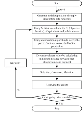
The MOGA based algorithm in this study follows the study of Feng et al.共1997兲, named as the cMOGA. Fig. 1 shows the main procedure of the cMOGA. The population of supply discounting ratios of agriculture and industry is first randomly generated by a binary code. Then the SIs for the two sectors, respectively, are evaluated for each chromosome by the proposed SOWA model.
This procedure next applies a proposed enumeration algorithm to derive the Pareto front and convex hull of the population共Feng et al. 1997兲. The Pareto front of the population can be mathemati-cally expressed in terms of noninferior solutions. If Solution S1 is better than S2 in terms of all objective values, Solution S1 domi-nates S2. If Solution S1 domidomi-nates any other solutions in the population, Solution S1 is a noninferior solution. The set of non-inferior solutions is the Pareto front of the population. The convex hull denotes a convex boundary composed by a set of linear seg-ments and enclosed by all feasible solutions. Fig. 2 shows the convex hull and the Pareto front. The convex hull is derived from the Pareto front.
Start
Generate initial population of supply discounting rate randomly
gen=0
Using SOWA to evaluate the SI (objective function) of agriculture and public sectors
Using enumeration algorithm to derive the pareto front and convex hull of the
population
Determine fitness value by calculating minimum distance between each
chromosome and segment
Is the stopping criteria satisfied? Reserving the elitists No
Stop Yes Selection, Crossover, Mutation gen=gen+1
Fig. 1. Flowchart of the cMOGA model
Based on the study of Feng et al. 共1997兲, fitness for each chromosome equals the shortest distance between the convex hull and the chromosome. The fitness is computed according to
fi= min共dij兲 共4兲
where fi= fitness value of the ith chromosome, and dij= shortest distance between the ith chromosome and the jth segment 共Fig. 2兲.
After defining the fitness value of each chromosome, the next step generates offspring of the generation through selection, crossover, and mutation. Those operations are similar to a con-ventional simple genetic algorithm. This work applies a tourna-ment method with pairwise fitness comparison for offspring selection, and a chromosome with a lower fi value has higher priority to be selected as offspring.
To further change offspring attributes, crossover and mutation operations were performed. Furthermore, this study applies the elitism approach to preserve the best solutions through genera-tions and to speed up convergence. The procedure is repeated until achieving convergence. Convergence is the variation ratio 共VR兲 between two generations less then 5% for ten consecutive generations. The VR is defined as
VRi+1=
冉
1 −num共Pi+1艚 Pi兲 num共Pi+1兲
冊
⫻ 100% 共5兲
where the subscript i denotes the ith generation; Pi= set of noninferior solutions for the ith generation; num共 兲=operator to calculate the number of set members;艚=operator of intersection; and VRi+1= variation ratio of the noninferior solution between the
ith and共i+1兲th generations.
SOWA Model
Simulation models 共e.g., the HEC-5 model兲 have been success-fully used in water allocation problem. However, recent studies have tended toward incorporating an optimization scheme into the simulation model to perform certain degrees of optimization. 共Wei and Hsu 2008兲. These optimization schemes typically in-clude the DP, LP, or NLP 共Yeh and Labadie 1997; Yang et al. 1996; Labadie 2004兲. Choosing an optimization model depends on the considering system characteristics共Tu et al. 2003兲. LP has been widely adopted for water allocation systems共Wei and Hsu 2008; Sun et al. 1995; Fredericks et al. 1998兲.
This study also uses LP to optimally allocate the water to different water-demand sectors. Instead of optimizing globally in
time, LP computes the optimal release at each time step for a model called the SOWA model. The model can allocate water to various water-demand sectors共such as agriculture and public sec-tors兲, while preserving an in-stream ecological base flow.
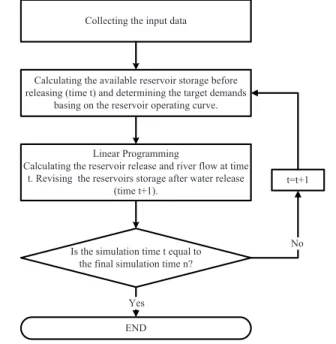
Fig. 3 shows the flowchart of the SOWA model. The input data should first be prepared for the simulation model. Those data include the inflow, demand, and capacity of hydraulic facilities, etc., collected from related project reports of the Water Resources Agency in Taiwan. Second, although each water use sector has its required water demand, the water-demand target should be ful-filled at each time step depending on the reservoir operating rules. The reservoir operating rule is applied to determine the target water demand of each water use sector according to the demand discounting ratio and reservoir storage before releasing. Third, based on the proposed formulation 共objective function and con-straints兲, this work use linear program is to compute the reservoir releases and the associated river flow at each time step. The res-ervoir storage is revised after the resres-ervoir releases. The proce-dure is repeated until the simulation time t is equal to the final time step. The LP model is the major computing routing in the third step. The following illustrates the detailed description of the model.
Objective Function of SOWA
The objective function of the linear model in SOWA at each time step t can be shown as
Zt= min
再
冉
兺
i苸ND WSH,iSHi t冊
+冉
兺
F苸NF WG,FGF t冊
+冉
兺
j苸NS WSP,jXSP,j t冊
冎
WSH,i⬎ WG,F⬎ WSP,J 共6兲The first term共SHit兲 of objective function denotes the water short-age of demand i. Minimizing the demand shortshort-age implies fulfill-ing the water demand as much as possible. The second term共Gtf兲 of the objective function denotes the discrepancy of water-level index among different reservoirs. Minimizing the index discrep-ancy implements the principle of “balanced water-level index” proposed in the HEC-5 developed by the U.S. Army Corps of
Fig. 2. Trade-off curve, convex hull, and fitness calculation
Collecting the input data
Calculating the available reservoir storage before releasing (time t) and determining the target demands
basing on the reservoir operating curve.
Linear Programming
Calculating the reservoir release and river flow at time t. Revising the reservoirs storage after water release
(time t+1).
Is the simulation time t equal to the final simulation time n?
END
t=t+1
No
Yes
Fig. 3. Flowchart of the SOWA model
Engineers. The formulary definition of Gftis defined in constraint 共8兲. The last term 共XSP,j
t 兲 of the objective function is the remaining reservoir vacancy. Minimizing vacancy is storing the water in reservoirs as much as possible. The weighting parameters WSH,i, WG,F, and WSP,Jrepresent the priorities of their associated objec-tives; the higher the values, the greater the objective importance.
Constraints of SOWA
Continuity Equations
Sit+1= Sit+
兺
Iit− Eit−兺
Xit− OFit∀i 苸 Ns 共7兲
Eq. 共7兲 is the continuity equation for reservoir water storage, where Sit+1 and S
i
tdenote the storages of reservoir i at t and t + 1 time step, respectively; Iit, Eit, Xit, and OFitare the inflow, evapo-ration, outflow, and overflow for reservoir i at time step t, respec-tively; and Nsis the set of all reservoirs. The continuity equations for other system nodes such as weirs and river conjunctions are similar to Eq.共7兲 but the Sit+1, Sit, and OFitequal to zero. Institutional Constraints
Sit−兺k苸NiXi,kt − LAYi,nt
LAYi,t共n+1兲− LAYi,nt + GF t =Sj
t−兺
l苸NJXj,lt − LAYj,nt
LAYtj,共n+1兲− LAYtj,n
∀i, j 苸 NS, ∀ k 苸 Ni, ∀ l 苸 Nj, ∀ F 苸 NF 共8兲 where GFt denotes the discrepancy of water-level index among different reservoirs at time step t; Xi,kt 共Xj,lt 兲 denotes the outflow withdrawing from reservoir i共j兲 to demand k共l兲 at time step t; LAYi,nt 共LAYj,nt 兲 indicates the nth operation zone of reservoir i共j兲 at time step t; LAYi,t共n+1兲共LAYtj,共n+1兲兲 indicates the 共n+1兲th opera-tion zone of reservoir i共j兲; Ni= set of all demands that were sup-plied by reservoir i; and Nj= set of all demands that are supplied by reservoir j. Eq. 共8兲 refers to the principle of balance water-level index for increasing the long-term water allocation perfor-mance for a multireservoir system. The balance water-level index method is an extension of rule curve operation for a single reser-voir and each reserreser-voir has to divide its volume into several op-erational zones before applying the method.
Ecological Base Flow Constraint Ri,jt ⱖ min
冉
兺
m苸⌸i,j
Imt,Bi,jt
冊
共9兲Eq.共9兲 represented the constraint of in-stream ecological base flow that needs to be fulfilled at each time step, where Ri,jt = ecological base flow to be fulfilled in river section共i, j兲 at time step t; Imt = mth inflow upstream of river section 共i, j兲; and Bi,jt = ecological base flow demand. The value of Bk,tis equal to Q95,
which means the river flow has 95% of the opportunities greater than discharge Q95.⌸i,jdenotes the set of all inflows upstream of river section共i, j兲. Eq. 共9兲 indicates that the ecological base flow demand will be fulfilled if there is enough upstream inflow for the river section. Otherwise, the base flow will be the summation of the upstream inflows.
Water Balance at Demand Node Djt=
兺
i苸⌳
Xi,jt + SHtj, ∀ j 苸 ND 共10兲 where Djt= target demand of demand node j at time step t; X
i,j t denotes the outflow withdrawing from node i and supply to de-mand j at time step t; SHtj= water shortage of demand node j; N
D denotes the set of all demand nodes; and⌳ indicates the set of all outflows that supply to node j.
Capacity Constraints
Capacity constraints define the capacity of reservoir storage, channels, pipes, and water treatment plant. The reservoir storage ranges from full capacity 共Su,i兲 to dead storage 共Sd,i兲 over the planning horizon and can be represented as follows:
Sd,iⱕ Si tⱕ S
u,i, ∀ i 苸 NS 共11兲
The water supply is subjected to the pipe capacity, and can be represented as
0ⱕ Xitⱕ Pit, ∀ i 苸 NP 共12兲 where Xitdenotes the pipe flow i at time step t; P
i
t= pipe capacity
i at time step t; and NP= set of all pipes.
Moreover, the water supply is also subjected to the capacity of water treatment plant, and can be represented as
0ⱕ
兺
j苸NUiXi,jt ⱕ Ujt 共13兲
where Xi,jt denotes the water supply to demand j from water treat-ment plant i at time step t; Utj= capacity of water treatment plant
j at time t; and NUi= set of demands supplied from water
treat-ment plant i.
Case Study
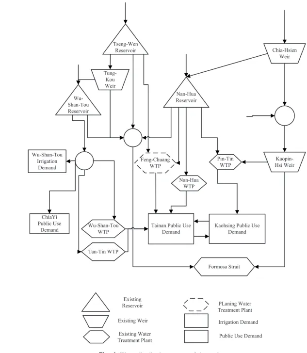
This study applies a hybrid model to manage and operate a com-plex real-world multireservoir system. The study region covers two metropolitan areas, Tainan and Kaoshing, and part of ChiaYi County in Southern Taiwan. Fig. 4 shows the water distribution system. The main water sources derive from the Nan-Hua Reser-voir, the Tseng-Wen ReserReser-voir, the Wu-Shan-Tou ReserReser-voir, and the Kaopin-Hsi Weir. Among these facilities, the Kaopin-Hsi Weir is located downstream from the KaoPin River and the others are situated in the Tseng-Wen river basin. The Nan-Hua Reservoir draws KaoPin river basin water through the Tung-Kou Weir. Four main existing water treatment plants and one planning water treat-ment plant are located in Southern Taiwan: the Pin-Tin water treatment plant, the Nan-Hua water treatment plant, the Wu-Shan-Tou water treatment plant, the Tan-Tin water treatment plant, and the Feng-Chuang water treatment plant, respectively. The basic water distribution principle is to use water from the Kaopin-Hsi Weir first, then from the other three reservoirs.
The other operating rule is to sequentially fulfill the demands depending on the water source withdrawn. For water withdrawn from the Kaopin River, the Kaoshing public use demand has higher priority over the Tainan public use demand; for water with-drawn from three reservoirs, the water supply priority is to meet the Wu-Shan-Tou irrigation demand, the Tainan public use de-mand, and the Kaoshing public use demand in sequence. The public use demand includes water for domestic and industrial uses. The three reservoirs operate together as a multireservoir
system, and the amount of water released from each reservoir is managed according to the balanced water-level index provided by the U.S. Army Corps of Engineers.
Reservoir operation should also be based on the operating curve of an equivalent reservoir. The operating curve is based on the equivalent reservoir combined with the Tseng-Wen Reservoir and the Wu-Shan-Tou Reservoir. The operating curve varies by months according to the changes in meteorological and hydro-logic conditions共Fig. 5兲. The operating curve divides equivalent reservoir volume into four operating zones; they are low buffer zone, high buffer zone, conservation zone, and flood control zone. Each zone has different criteria for decreasing target demand, depending on how much water has been stored in the equivalent reservoir.
This study includes four decision variables, which are the weightings共supply discounting ratio兲 at high buffer zone and low buffer zone for agriculture and public use. The decision variables
Tseng-Wen Reservoir
Nan-Hua Reservoir
Tainan Public Use Demand
Kaohsing Public Use Demand Wu-Shan-Tou Reservoir Nan-Hua WTP Pin-Tin WTP Formosa Strait Wu-Shan-Tou Irrigation Demand Wu-Shan-Tou WTP ChiaYi Public Use Demand Feng-Chuang WTP Tung-Kou Weir Chia-Hsien Weir Kaopin-Hsi Weir Existing Reservoir Existing Weir Existing Water Treatment Plant PLaning Water Treatment Plant Irrigation Demand
Public Use Demand Tan-Tin WTP
Fig. 4. Water distribution system of the study area
0 10000 20000 30000 40000 50000 60000 70000 1 3 5 7 9 11 13 15 17 19 21 23 25 27 29 31 33 35 Time(ten-days) Storage (1000 cu bi c meter ) Flood control
Conservation Low Buffer High Buffer
Fig. 5. Definition of the reservoir operating zone for the equivalent reservoir of Tseng-Wen Reservoir and Wu-Shan-Tou Reservoir
must be coded as chromosomes and each decision variable is coded as eight binary bits. Because the agriculture and public sector have different degrees of enduring deficit abilities, the weighting range should be set differently. The weighting range of agriculture use is set from 0.3 to 1 in this study and the weighting range of public use is set from 0.5 to 1. The weighting at the high buffer zone should be larger than the weighting at the low buffer zone. Hence the weighting range at the low buffer zone for culture and public use should be revised as from 0.3 to the agri-culture weighting value of the high buffer zone and from 0.5 to the public weighting value of the high buffer zone, respectively.
Results and Discussion
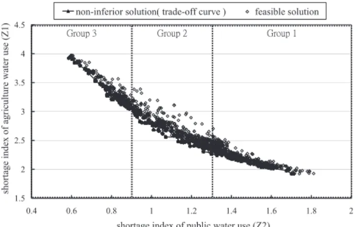
Fig. 6 presents the trade-off curve for the SI of agriculture water use共Z1兲 and SI of public water use 共Z2兲 computed by cMOGA. The noninferior solutions were obtained after 208 generations with a population size of 200, and the convergence criterion is that VR is less then 5% for ten consecutive generations共Fig. 7兲. Fig. 6 indicates that the minimum SI of agriculture water use is approximately 1.98 when the maximum SI of public water use is 1.70. On the other hand, the maximum SI of agriculture water use is 3.93 when the minimum SI of public water use is approxi-mately 0.59. For all noninferior solutions, the SI of agriculture water is always higher than that of public water. This situation is
caused because agriculture water can only be supplied by the Tseng-Wen Reservoir and the Wu-Shan-Tou Reservoir but the public use water has other water sources, the Kaopin-Hsi Weir, the Chia-Hsien Weir, and the Nan-Hua Reservoir共refer to Fig. 4兲. Fig. 7 displays the distribution of decision variables’ value for noninferior solutions to explore their structure. Each feasible so-lution has four decision variables, the discounting ratios for agri-culture and public water use at the high buffer zone 共C1,1 and C2,1兲 and those at the low buffer zone 共C1,2and C2,2兲. The first
suffix of variables denotes water use type and the second suffix represents different buffer zones. Fig. 7 clearly shows that the distribution of discounting ratios for the two buffer zones is sepa-rated into two groups. As expected, the low buffer zone distribu-tion is enclosed by the distribudistribu-tion at the high buffer zone. The discounting ratios for the low buffer zone clusters near the lower left corner with C1,2 range roughly between 0.3 and 0.7, and C2,2range roughly between 0.5 and 0.65. The discounting ratios
for the high buffer zone distribute are much more scattered than those of the low buffer zone, which is discussed further in the following.
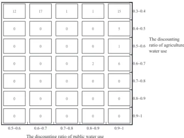
The study divides the noninferior solutions into three groups, depending on the objective values共Fig. 6兲 to analyze the relation-ship among objectives and decision variables. The first group em-phasizes the agriculture water demand; therefore, it has the higher end of the range for the public SI 共1.328–1.702兲 and the lower end of the range for agriculture SI 共1.978–2.242兲. The second group equally emphasizes the public and agriculture water de-mands, and the SI value ranges are 0.884–1.328 and 2.242–3.057, respectively. The third group emphasizes the public water de-mand; thus, it has the lower end of the range for the public SI 共0.586–0.884兲 and the higher end of the range for the agriculture SI共3.057–3.927兲.
Figs. 8–10 show the occurrence frequency for discounting ra-tios of agriculture and public water use with respect to different groups. A higher value of discounting ratio indicates a higher priority for fulfilling the associated water demand. For the high buffer zone and the low buffer zone, the discounting ratios of agriculture for the first group共Fig. 8兲 concentrate on higher value than those for the third group共Fig. 10兲. The discounting ratios of public water demand for the first group are expected to concen-trate on the lower value than that for the third group. However, the result is not as clear as that for agriculture. For the low buffer 1.5 2 2.5 3 3.5 4 4.5 0.4 0.6 0.8 1 1.2 1.4 1.6 1.8 2
shortage index of public water use (Z2)
sh ortage in d ex o f agr icu lture water use (Z1 )
non-inferior solution( trade-off curve ) feasible solution Group 3 Group 2 Group 1
Fig. 6. Trade-off curve between the SI of agriculture water and that of public water共final population兲
0.5 0.6 0.7 0.8 0.9 1 0.3 0.4 0.5 0.6 0.7 0.8 0.9 1
The discounting ratio of agriculture water use
The discou ntin g rati o o f p ub lic water u se
The discounting ratio at High Buffer Zone The discounting ratio at Low Buffer Zone
Fig. 7. Distribution of discounting ratios for the two buffer zones
0.3~0.4 0.4~0.5 0.5~0.6 0.6~0.7 0.7~0.8 0.8~0.9 0.9~1 0.5~0.6 0.6~0.7 0.7~0.8 0.8~0.9 0.9~1 0 16 9 5 0 1 3 0 0 0 0 2 1 1 0 0 0 0 1 8 4 0 0 0 0 0 0 0 0 0 0 0 2 4 3 The discounting ratio of agriculture water use
The discounting ratio of public water use
Fig. 8. Occurrence frequency distribution of discounting ratios for the first group
zone, as expected, C2,2for the first group concentrates more on
the lower value than that of the third group. Nevertheless, for the high buffer zone, although C2,1for the third group still
concen-trates on high value as expected共Fig. 10兲, C2,1for the first group does not concentrate on low value but varies widely in the fea-sible range共0.5–1兲 共Fig. 8兲.
The water supply system structure shown in Fig. 4 explores the exception for C2,1 when emphasizing agriculture water
de-mand. Fig. 4 indicates that only two reservoirs共Tseng-Wen Res-ervoir and Wu-Shan-Tou ResRes-ervoir兲 supply the agriculture demand 共Wu-Shain-Tou irrigation demand兲, while the public water demands共Tainan and Kaoshing, and part of ChiaYi County public demand兲 can be supplied by all five major water sources 共Tseng-Wen, Wu-Shan-Tou, Nan-Hua Reservoir, and Kaopin-Hsi, Chia-Hsien Weir兲. The system structure induces that, when water level is in the high buffer zone, the public demands withdraw from their independent water sources 共Kaopin-Hsi Weir, Chia-Hsien Weir, and Nan-Hua Reservoir兲 and do not struggle for the water stored in Tseng-Wen and Wu-Shan-Tou Reservoirs with the agriculture demand. This does not force the discounting ratio of public water demand to low value and induces the discounting
ratio of public water demand to vary widely in its feasible region even with emphasizing agriculture demand 共shown as Fig. 8兲. However, when the water level drops in the low buffer zone in severe dry season, with supplying less water to the public demand from Kaopin-Hsi Weir, Chia-Hsien Weir, and Nan-Hua Reservoir, it will induce public water use and agriculture water use to struggle for the limited water stored in the Tseng-Wen and Wu-Shan-Tou Reservoirs. Hence, emphasizing agriculture water de-mand forces the discounting ratio of public water dede-mand to low value共shown as Fig. 8兲.
Fig. 9 indicates that, when equally emphasizing agriculture and public demand, the discounting ratios for both water demands vary in the same trend. The high buffer zone trend slightly re-stricts the water-demand supply共both C1,1and C2,1range between
0.9 and 0.1兲. the low buffer zone trend severely restricts the water-demand supply 共C1,2ranges between 0.3 and 0.4 and C2,2
ranges between 0.5 and 0.6兲.
Conclusions
To overcome the limitations of using conventional multiobjective optimization methods to solve water sharing conflict problems, this paper develops a novel multiobjective hybrid model that in-tegrates a cMOGA with a rule curve based reservoir operation model共SOWA兲. The study applies the proposed model to solve the conflict between different water use sectors. The proposed hybrid model generates different alternatives in a single run, in-creasing the efficiency of obtaining noninferior solutions 共trade-off curve兲. The case study demonstrates that the proposed model solves a practical multiobjective water resource planning prob-lem. The discounting ratios of noninferior solutions provide rel-evant information to facilitate stakeholders negotiating under different preferences. The results also reveal how the decision makers’ preference influences the discounting ratios of difference water use. When decision makers prefer agriculture use to public use, the discounting ratio of public use at the low buffer zone should be limited on the lower bound. The discounting ratio of agriculture use at the low buffer zone should, however, be limited on the lower bound when decision makers prefer public use to agriculture use. Without particular preference, the discounting ra-tios of agriculture use and public use at the low buffer zone both should be limited on the lower bound. Therefore, stakeholder preference is also an important factor for a multiobjective water resource allocation problem.
References
Cieniawski, S. E., Eheart, J. W., and Ranjithan, S.共1995兲. “Using genetic algorithms to solve a multiobjective groundwater monitoring prob-lem.” Water Resour. Res., 31, 399–409.
Cohon, J. L., and Marks, D. H.共1977兲. “Review and evaluation of mul-tiobjective programming techniques—Reply.” Water Resour. Res., 13, 693–694.
Feng, C. W., Liu, L. A., and Burns, S. A.共1997兲. “Using genetic algo-rithms to solve construction time-cost trade-off problems.” J. Comput.
Civ. Eng., 11共3兲, 184–189.
Fredericks, J. W., Labadie, J. W., and Altenhofen, J. M.共1998兲. “Decision support system for conjunctive stream-aquifer management.” J. Water
Resour. Plann. Manage., 124共2兲, 69–78.
Labadie, J. W. 共2004兲. “Optimal operation of multireservoir systems: State-of-the-art review.” J. Water Resour. Plann. Manage., 130共2兲, 93–111. 0.3~0.4 0.4~0.5 0.5~0.6 0.6~0.7 0.7~0.8 0.8~0.9 0.9~1 0.5~0.6 0.6~0.7 0.7~0.8 0.8~0.9 0.9~1 16 5 0 0 0 0 0 9 0 0 0 0 0 0 0 0 0 0 0 0 0 0 0 0 0 0 0 0 0 0 3 2 0 0 25 The discounting ratio of agriculture water use
The discounting ratio of public water use
Fig. 9. Occurrence frequency distribution of discounting ratios for the second group
0.3~0.4 0.4~0.5 0.5~0.6 0.6~0.7 0.7~0.8 0.8~0.9 0.9~1 0.5~0.6 0.6~0.7 0.7~0.8 0.8~0.9 0.9~1 12 0 0 0 0 0 0 17 0 0 0 0 0 0 1 0 0 0 0 0 0 1 0 0 2 0 0 0 15 5 1 6 0 0 0 The discounting ratio of agriculture water use
The discounting ratio of public water use
Fig. 10. Occurrence frequency distribution of discounting ratios for the third group
Lund, J. R., and Israel, M. 共1995兲. “Water transfers in water-resource systems.” J. Water Resour. Plann. Manage., 121共2兲, 193–204. Lund, J. R., and Reed, R. U.共1995兲. “Drought water rationing and
trans-ferable rations.” J. Water Resour. Plann. Manage., 121共6兲, 429–437. Prasad, T. D., and Park, N. S.共2004兲. “Multiobjective genetic algorithms for design of water distribution networks.” J. Water Resour. Plann.
Manage., 130共1兲, 73–82.
Sun, Y. H., Yeh, W. W. G., Hsu, N. S., and Louie, P. W. F. 共1995兲. “Generalized network algorithm for water-supply-system optimiza-tion.” J. Water Resour. Plann. Manage., 121共5兲, 392–398.
Tu, M. Y., Hsu, N. S., Tsai, F. T. C., and Yeh, W. W. G.共2008兲. “Opti-mization of hedging rules for reservoir operations.” J. Water Resour.
Plann. Manage., 134共3兲, 3–13.
Tu, M. Y., Hsu, N. S., and Yeh, W. W. G. 共2003兲. “Optimization of reservoir management and operation with hedging rules.” J. Water
Resour. Plann. Manage., 129共2兲, 86–97.
Wei, C., and Hsu, N. 共2008兲. “Multireservoir real-time operations for flood control using balanced water level index method.” J. Environ.
Manage., 88, 1624–1639.
Yang, C., Chang, L., Yeh, C., and Chen, C.共2007兲. “Multiobjective plan-ning of surface water resources by multiobjective genetic algorithm with constrained differential dynamic programming.” J. Water Resour.
Plann. Manage., 133共6兲, 499–508.
Yang, S. L., Hsu, N. S., Louie, P. W. F., and Yeh, W. W. G.共1996兲. “Water distribution network reliability: Stochastic simulation.” J. Infrastruct.
Syst., 2共2兲, 65–72.
Yeh, C. H., and Labadie, J. W.共1997兲. “Multiobjective watershed-level, planning of storm water detention systems.” J. Water Resour. Plann.
Manage., 123共6兲, 336–343.