ON ESTIMATION AND PREDICTION PROCEDURES FOR AR(1) MODELS WITH POWER TRANSFORMATION

Journal

of

Forecasting, Vol. 12, 499-511 (1993)

On Estimation and Prediction Procedures

for

AR(1)

Models with Power

Transformation

J.

C.

LEE* and S. L. TSAO

National Chiao Tung University, Hsinchu, Taiwan and

AT& T Bell Laboratories, Holmdel, NJ, U. S.A.

ABSTRACT

The power transformation of Box and Cox (1964) has been shown to be quite useful in short-term forecasting for the linear regression model with AR(1) dependence structure (see, for example, Lee and Lu, 1987, 1989). It is crucial to have good estimates of the power transformation and serial. correlation parameters, because they form the basis for estimating other parameters and predicting future observations. The prediction of future observations is the main focus of this paper. We propose to estimate these two parameters by minimizing the mean squared prediction errors. These estimates and the corresponding predictions compare favourably, via revs and simulated data, with those obtained by the maximum likelihood method. Similar results are also demonstrated in the repeated measurements setting.

KEY WORDS AR( 1) dependence Box-Cox transformation Maximum

likelihood Minimum prediction errors Simulations Technology penetration

INTRODUCTION

Through scientific discoveries and evolution, new products spread and grow to replace existing ones. This process is called technological substitution. Thus, as technology advances, steam/motor merchant vessels replace sail merchant vessels, colour televisions replace black- and-white televisions, digital telephone switching systems replace analog switching systems. The rate of the change, called technology penetration, is defined as the ratio of the number

of

new products to the combined total of new and old products. The penetration data tend to follow an S-shaped curve and exhibit very strong positive first-order autoregressive (or

AR(1)) dependence. The S-shaped curve is typical in many types of growth curve models, such as Gompertz and logistic, among others. However, a typical growth curve such as Gompertz

* Research supported in part by NSC grant 82-208-M009-054

0 1993 by John Wiley & Sons, Ltd.

0277-6693/93/060499-13$11 .SO Received January 1992

500 Journal of Forecasting Vol. 12, Zss. No. 6 or logistic is not quite adequate in forecasting penetration at a future time. T o illustrate the point, let F ( t ) be the technology penetration at time t . Then if a logistic curve is assumed, we expect log(F(t)/(l

-

F ( t ) ) ) to be linear in time, i.e. a linear growth function. But when dealing with real data, we often found that the more flexible transformation of Yr = F(t)/(l

-

F ( t ) )

gives much superior predictive accuracies. This is, perhaps, primarily due to the fact that the linearity assumption for the growth function can be enhanced considerably with the Box-Cox power transformation, along with the incorporation into the model of the proper dependence structure among the observations. For more details, see Lee and Lu (1987). Nevertheless, the maximum likelihood estimation method used by Lee and Lu (1987) could produce undesirable estimates to result in a poor forecast when the sample size is small. Therefore we propose in this paper a n intuitively appealing method to deal with the prediction of future observations in small samples.

A family of data-based transformed models for forecasting technological substitutions has been empirically shown t o be quite useful for short-term forecasts (see Lee and Lu, 1987,

1989). These models are more general and include as special cases the four well-known S-shaped growth curve models: Gompertz, logistic, normal, and Weibull. The transformation needed depends on the data at hand. Basically, the widely used Box-Cox (1964) transformation is applied to the AR(1)-dependent data. More specifically, let YI,

...,

YT be a set of T observations. The transformation is defined as

when A Z 0 y p = h

when A = 0

where y is a known constant such that Y,

+

y

>

0 for all t . In practice, y = 0 if all Yr’s are positive. Furthermore, Y,“)(t = 1 ,

...,

T ) are assumed to be normally distributed with the mean linear in the regression parameters and the covariance matrix C = a‘V11, V I ~ = ( C a b ) , ~ ~ b = p l ‘ - ~ I , for a, b = 1 ,

...,

T , and -1

<

p

<

1 . In other words,

YCA) = ( Y p ,

...,

Yf”)’

=

x g +

E _{( 2 )}

where Xfl is the growth function,

is=

( a ,

p ) ’ , X is the design matrix with 1’s in the first

column and tl,

...,

t~ or log(tl),

...,

log(tT) in the second column, depending on the growth curve model being considered (see Lee and Lu, 1987). The vector of disturbance terms E is

assumed to distribute as a multivariate normal with mean vector 0 and covariance matrix a2V11. If a higher-degree polynomial is assumed for the growth function, the dimensions of

X

and

fl

are adjusted accordingly. For example, if a second-degree polynomial in time is assumed for the growth function, then the third column of

X

is t : to tf. Model (2) has also been proved useful by Fiebig and Bewley (1987) in forecasting demand for international communications services as well as for other types of data.

The Box-Cox transformation has been considered for the general time series by several authors, including Granger and Newbold (1976), Hopwood et al. (1984), and Pankratz and Dudley (1987), among others. However, none of the above authors discussed the estimation of parameters from a prediction point

of

view. Model (2) has been extended to the situation in which several concurrent short time series are available (see Keramidas and Lee, 1990). We will discuss this extended model in

more

detail in the next section while the rest of this section is devoted to the single-series situation.

Let y, of dimension

k

x 1 , be the vector of future observations to be predicted on the basis of the past observations

Y

= ( Y I ,

...,

YT)’ such that E ( y ( ” ) = xfl where x is the design matrix corresponding to the future observations. Furthermore, Cov(Y(’)’, y(’)‘)’ = a2 (Cab), where

J . C. Lee and S. L . Tsao Power Transformation 501 estimates (MLEs), the forecasts of y, which is obtained from the conditional expectation of y(’) given Y, can be written as

(3)

where

s=

( X f 6 i 1 1 X ) - ’ X ’ ~ i 1 1 Y ~ ~ ) , jj = @, j2,

...,

4 k ) ’ ,

1 = (1,

...,

1)’, 611 = (&,b),

& 6 = $ u - 6 ’ , X r and Y p ) are the Tth row of X and Ycx), respectively, and

^x

and j are the

MLEs of X and p , respectively; z = (zl,

...,

zk)’, z d = (zf,

...,

z?)‘, for any constant d , and exp(z) = (exp(zl),

...,

exp(zk))’. For the remainder of the paper we will concentrate on the special case in which

k

= 1, i.e. we are interested only in a one-step-ahead forecast. This is due to our belief that a one-step-ahead forecast is less speculative and hence is more reliable for

the purpose of comparing different methods.

The prediction of future observations y is the main focus of this paper. The forecasts

9 ,

of

y, depend very crucially on the quality of the estimates

^x

and

8.

The MLEs of these two parameters have been used with some success by Lee and Lu (1987). Nevertheless, the method could produce undesirable estimates when the sample size is relatively small, as the MLEs are optimal in large samples only. This will in turn render poor forecasts in small samples.

The purpose of this paper is t o propose an intuitively appealing method, minimum prediction error (MPE), for estimating these two parameters and to explore possible advantages of using this estimation method in the prediction of future observations. The MPE method, formulated t o some extent in the spirit of Rissanen’s (1986) accumulated prediction errors method and Lee’s (1988) minimum prediction variance estimate, is more sensitive than the traditional MLEs to the prediction of future observations. Moreover, it is less dependent on the distributional assumption imposed on the observations, as it minimizes the mean squared prediction errors.

Since the MPE method will not give closed-form representations for the parameter estimates, only empirical comparisons of the proposed method with the maximum likelihood method will be made in terms of the predictive accuracy of future observations. These comparisons are made in both real and simulated data. In addition, empirical comparisons for the parameter estimates by both methods wilI also be made via simulation.

Details of the proposed method are given in the next section. Empirical comparisons in both real data and simulations are presented in the third section. Conclusions are given in the final section. (1

+

~ [ X S

+

ij(Y$)

-

X d ) ]

)”’

-

y e x p [ x g + i j ( ~ P - X d ) ] - 7 when

^x

# 0 when

^x

= 0

4 =

[

MINIMUM PREDICTION ERROR ESTIMATES

In this section we will consider the MPE method for a single series as well as for several concurrent short series, with the emphasis on the single-series situation.

A single series

In equation (3) the MLpEs of X and p are obtained by maximizing the profile log-likelihood function (see Lee and Lu, 1987), which is defined as

T

( T - l ) log(1 - p Z ) (41

where G2(X, p ) = (l/T)(Y(”

-

Xg(X, p))’VII1(Y(’) - Xfi(X, p ) ) and

b(X,

p ) is the

g,

given in equation (3), with

^x

and j replaced by X and p, respectively. The reason for considering only the profile likelihood function of X and p is that, given X and p ,

b(X,

p ) and e2(X, p ) are

T

2 t = 1 2

502 Journal of Forecasting Vol. 12, Zss. No. 6

functions of X and p only. O n c e 1 and ,ij are obtained by maximizing 1 ( A , p ) , then B(A, {),

G2(X,

b ) ,

^x

and ,ij are the MLEs of

8,

0 2 , A, and p .

Instead of using the MLEs for these two parameters, we can treat

9 ,

defined in equation (3),

as a function of X and p , whose values are obtained by minimizing the mean squared prediction errors, More specifically, the predictions are made for Yt, t = 3,

...,

T, since we need at least two observations to estimate parameters in a simple linear model. In predicting Yt, the sample is Yr-1 = ( Y I ,

...,

Y f - 1 ) ’ . Thus, the predictions are made sequentially and the sample on which each prediction is based increases in size one at a time. The approach is prequential in nature in that predictions of future observations are made sequentially (see Dawid, 1984; Keramidas and Lee, 1990). The objective function to be minimized is

where

pf,

is defined in exactly the same form as

9,

given in equation (3), with

k

= 1, Treplaced by t - 1, x by X f , and

X

by

Xr-1,

the first t

-

1 rows of X.

The minimization of MSE1(X, p ) with respect to X and p can be facilitated by an optimization routine in the Port 3 Mathematical Subroutine Library (1984). We will use the version requiring both the first and the second derivatives of the objective function. These derivatives are provided in the Appendix.

Several concurrent short series

When several short time series are available, Keramidas and Lee (1990) extended model (2) to the general growth curve model with serial covariance structure for forecasting technological substitutions. The model is

Y ( h ) =

X

T

A

+

E (6)

T x N T x m m x r r x N ‘ T x N

where Ych) =

(Y

{’I),

...,

Y!$””),

Yl”’

= ( Y ! ? ) ,

...,

Y$?))’ with Y$’” defined as in model (1); 7 is unknown,

X

is the known design matrix characterizing the type of growth function, and A is the known design matrix characterizing the grouping among the N independent series into

r different curves. Furthermore, the columns of E are independent T-variate normal with mean

vector 0 and common covariance matrix a2V~l. For the rest of the paper we will consider a particularly practical situation in which there are only r different A’s. This means that we will apply the same power transformation to each of the observations in the same group. The MLpEs of X and p have been considered by Keramidas and Lee (1990).

For the MPE estimates of these parameters, we consider the following extended prediction problem. Let y, of dimension k x n, be a set of n(

6

N ) future k-dimensional observations whose previous T-dimensional observations are a subset of

Y.

Let x, of dimension k x m, be the design matrix corresponding to y, Y = (YI,

...,

YN), A = (AI,

...,

AN), y = ( y ~ ,

...,

y,,) and assume that for i

<

n,

J. C. Lee and S. L . Tsao Power Transformation 503

for a, b = 1,

...,

T +

k.

When the MLEs of

X

and p are used in place of these unknown parameters, the forecasts of y i is the same-as

9 ,

given in equation (3), with

^x

replaced by ^xi,

by i A i where

i =

( X ’ ~ ~ I I ~ X ) - ~ X ’ ~ ~ I I Y ~ ) A ’ ( A A ’ ) - ~ .

As in the single-series situation, we can treat the predictor 9i as

a

function of X i and p , whose estimates are derived by minimizing the mean squared prediction errors. Thus, the objective function to be minimized is

N T

MSEz(X, p ) =

C C

( Y i j - P i j ) * / ( T - m ) N (9) i = l j = m + l

The minimization of MSEz(X, p ) is similar to that of MSEl(X, p ) . The derivatives of MSEz(X, p ) can be obtained in exactly the same manner as those of MSEl (A, p ) and hence are omitted.

EMPIRICAL COMPARISONS

In this section we will compare empirically the predictive accuracy of the linear models in which the power transformation and serial correlation parameters are estimated by the maximum likelihood (ML) and the MPE methods. For real data examples, we will consider four sets of observations on technology penetration, three in telephone-switching systems and one in television receivers. Since in the area of technological substitutions the logistic growth curve (or Fisher-Pry model, 1971) is the most popular, we will confine our attention to this particular model. For the logistic curve, if F ( t ) is the new technology penetration at time t, then setting YI = F ( t ) / ( l - F(t)) we have Y!’’ = log(F(t)/(l

-

F(t))) when X = 0, which is exactly the logistic o r the Fisher-Pry model if the transformed variables are assumed independent. For the simulation study, however, we will be dealing with Yr directly and hence a particular growth curve is irrelevant to our discussion.

In order to compare the predictive accuracy when the unknown power transformation and serial correlation parameters are estimated by the ML and the MPE methods, we will employ three different measures: the mean absolute deviation (MAD), the mean absolute relative deviation (MARD), and the fraction of accurate prediction (FAP). The MARD is perhaps a better measure than MAD for real data examples because the time series observations are monotonically increasing and the comparison of forecasts is conducted in a sequential manner. On the other hand, for the simulation study, we will fix the sample size and hence only MAD and FAP are employed for the comparison purpose. The definition of FAP is simply the fraction with more accurate forecast for a given method. We next define the other two measures.

Let E ( t ) be the forecast of the new technology penetration F ( t ) and e ( t ) = F ( t ) -

E ( t ) ,

for t = 1,

...,

a. Then the MAD and MARD are defined as

a

r = 1

MAD =

I

e ( t ) I/a (10)

’

The technology penetration is defined as the ratio of the number of new products to the combined total of new and old products.

504 Journal

of

Forecasting Vol. 12,

Iss.

No.

6

The above definitions are relevant for real data examples. For the simulation the corresponding definitions are easily seen by replacing F ( t ) by Yt and

P ( t )

by

fit,.

Real data with a single series

Two sets of technology penetration data, analysed by Lee and Lu (1987, 1989), are listed in Table I. We will consider the empirical comparison of the predictive accuracy in one-step- ahead forecasts between the two estimation methods for the power transformation and serial correlation parameters. Also, in the comparison the initial sample size is five, instead of eight as in the previous studies. The feasibility of estimating these two parameters in small samples is one of the features of the proposed method.

Table

I1

shows the comparison of the predictive accuracy in terms of the three measures mentioned earlier. In terms of MARD, the improvements (IMP) of the forecasts based on the

MPE

method over the ML method for these two parameters are 27% for the TV data and 51%

for the telephone data. The corresponding improvements in terms of MAD are 11 070 and 33%,

Table I. Technology penetration data

~ ~~ ~

Colour TV receivers Telephone-switching systems

Year Penetrations Year Penetrations

1955 1956 1957 1958 1959 1960 1961 1962 1963 1 964 1965 1966 1967 1968 1969 1970 1971 1972 1973 1974 1975 1976 1977 1978 1979 1980 1981 1982 1983 1984 1985 0.00016 0.00052 0.00219 0.00394 0.00569 0.00743 0.00943 0.01208 0.01889 0.03 120 0.05332 0.09694 0.16325 0.24 1 75 0.32034 0.35744 0.41015 0.48631 0.55355 0.6225 1 0.68394 0.73606 0.77065 0.77984 0.80926 0.83028 0.82916 0.87595 0.88703 0.90465 0.91519 1965 1966 1967 1968 1969 1970 1971 1972 1973 1974 1975 1976 1977 1978 1979 1980 1981 O.ooOo9 o.oO015 0.00157 0.00707 0.01205 0.02234 0.03578 0.05746 0.08495 0.11700 0.14995 0.18482 0.23308 0.28858 0.35238 0.42244 0.47951

J . C. Lee and

S.

L. Tsao Power Transformation 505 Table 11. Comparison of one-step-ahead forecast accuracy for two single series

Colour TV receivers Telephone-switching systems

MPE ML IMP(%) MPE ML IMP(%)

MAD 0.01 12 0.0126 11 0.0061 0.0090 33

MARD 0.0586 0.0800 27 0.0383 0.0788 5 1

FAP(%) 73 27 67 33

respectively. Meanwhile, for the MPE method, the FAP achieves 73% for the TV and 67%

for the telephone data. These improvements are indeed impressive.

Real data with several concurrent short series

The two data sets (Regions A and B), given in Tables 1 and 4 of Keramidas and Lee (1988), are used here for the comparison of the predictive accuracy of the two estimation methods for the power transformation and serial correlation parameters. Region B was further analysed in Keramidas and Lee (1990).

In the comparison the initial sample sizes for Regions A and B are 3 and 4, respectively. The higher initial sample size for Region B reflects the inclusion of the quadratic growth function. In Region A only a linear growth function is used while both the linear and the quadratic growth functions are explored for Region B. It is found that only the linear growth function shows some improvement for the MPE estimates over the MLEs for Region B. Table 111

exhibits the comparison of the predictive accuracy in terms of MAD, MARD, and FAP. There are some improvement of the forecasts based on the MPE Method over the ML method. The improvement, however, is not as pronounced as in the single series studied earlier.

Simulation

The main focus of this section is

on

the simulation results for a single series. We will consider the comparison of the predictive accuracy of the forecasts based on both estimation methods. In addition, we will also consider the comparison of the estimates of the power transformation and serial correlation parameters.

In the simulation for a single series we have

where the disturbance terms &(t = 1,

...,

T ) are independent normal, Student’s t , or gamma,

Table 111. Comparison of one-step-ahead forecast accuracy for two sets of concurrent short series

Region A Region B

MPE ML IMP(%) MPE ML IMP(%)

~ ~~

MAD 0.0151 0.0198 24 0.0199 0.0216 8

MARD 0.0491 0.0336 32 0.0589 0.0620 5

506 Journal of Forecasting Vol. 12, Iss. No. 6

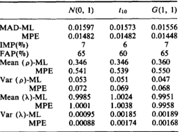
Table IV. Comparisons of one-step-ahead forecasts and parameter estimates for simulated data

MAD-ML M PE IMP(%) FAP( To) Mean (p)-ML Var (p)-ML MPE Mean (A)-ML Var (A)-ML M PE MPE MPE 0.01597 0.01482 7 65 0.346 0.541 0.053 0.072 0.9985 1 .0001 0.00095 O.Ooo88 0.01573 0.01482 6 60 0.346 0.539 0.05 1 0.069 1.0024 1.0038 0.00185 0.00174 0.01556 0.01448 7 65 0.360 0.550 0.047 0.068 0.9951 0.9958 0.00189 0.00168

each with mean o and variance u2. Also, G ( & , 02) denotes the gamma distribution with the shape parameter 81 and the scale parameter l/&, and t , denotes the Student’s t distribution with Y degrees of freedom. In the simulation, we set (IL = 0,

p

= 0.2, y = 0, u = 0.03, h = 1,

p = 0.85, and T = 20. The number of realizations of model (12) is lo00 for each distribution. Forecasts up to five steps ahead are performed and compared with the actuals. A summary of the comparisons of one-step-ahead forecast accuracy and parameter estimates are given in Table IV.

From this table it is evident that some improvement in one-step-ahead forecast accuracy has been achieved in terms of MAD and FAP. Improvements for higher step forecasts are similar. Also, there is clearly a significant improvement of the MPE estimate of the serial correlation over the MLE. This means that the MPE method could provide a viable alternative to the MLE of the serial correlation alone even when no power transformation is applied to a linear model with AR(1) dependence structure. This special situation is very important because the model is useful in time-series data. A more detailed comparison of the estimation of the serial correlation parameter by both methods is depicted in Figure 1 in which the distributions of the lo00 estimates of p by both estimation methods for normal, t10, and G ( l , 1) are shown. First,

the distributions of

b,

for a given estimation method, is essentially independent of the distributional assumption on the disturbance terms 6,. However, there is a significant difference in these distributions between the two estimation methods. Even though the true value of p is 0.85, its ML estimate never goes beyond 0.8, while the MPE estimate of p is between -1 and 1 . This explains why the variance of the MLEs is smaller than that of the MPE estimates.

Similar comparison of the estimation of the power transformation parameter by ML and MPE methods is depicted in Figure 2. There seems to be no significant difference between the two methods in estimating this parameter.

We note that when the power transformation parameter X is fixed at either 0 or 1 the results for the norlnal distribution are not much different from those presented in Table IV. Similar results are obtained when h = 0 but estimates of both X and p are made for the purpose of forecasting.

If p is restricted to [0, l), a possible situation in which the serial correlation is non-negative, the results for the one-step-ahead forecasts and parameter estimates are similar to those presented in Table IV. In general, the mean values

of

6

are larger while the variances are

Power Transformation

507 J. C. Lee

and

S. L .

Tsao

MPE ML MPE ML -1.0 ao 0.s 1.0 -1.0 ao 0.5 9.0 w 1.0 1.1 1 1 0.0 1.0 1.1 1 2 N(o.1) w.0 wo Wac) 4.0 0.0 0.5 1.0 -1.0 0.0 0.5 1.0 0.0 1.0 1.1 1 1 0.0 1.0 1.1 1 2 no no no tl0 -1.0 0.0 0.5 1.0 -1.0 0.0 0.5 1.0 0.B 1.0 1.1 12 0.0 1.0 1.1 12 w . 1 1 acl.$t W.1) GV.11

Figure 1 . Distributions of

Z

by MPE and ML

methods methods

Figure 2. Distributions of

^x

by MPE and ML

slightly smaller, because the negative values of are not allowed. The decrease in the size of the variance of

b

for each distribution is more appreciable in the ML method than in the MPE method, which may be an argument for considering only the nonnegative value for p , when the ML method is used.

CONCLUSIONS

From the real and simulated data we found that the minimum prediction error estimates of the power transformation and serial correlation parameters are viable alternatives to the MLEs

508 Journal

of

Forecasting Vol. 12,

Zss.

No. 6

of these two parameters. This is especially true with a single time series when the sample size is relatively small. For the situation in which several concurrent short time series are available, the results are still encouraging, even through they are not as convincing. Finally, it is emphasized that although all the real data are from the area of technological substitutions, the proposed method is useful for any type of data in which a power transformation of the dependent variable can be applied to a linear model with AR(1) dependence structure. The method is, of course, equally suitable when no power transformation is needed.

APPENDIX: THE DERIVATIVES OF MSEi(X, p )

In this appendix we will give the first and the second derivatives of the objective function

MSE1(X, p ) with respect to X and p.

2p - 1 - p

z

o

0 -1 - p 4p

...

J . C. Lee and

S.

L. Tsao Power Transformation 509

-

2x-2Pt[1

+

x P p ]

when A # 0 when X = O

5 10 Journal

of

Forecasting Vol. 12, Iss. No. 6

a2

a2

a 2

ax2

ax2

a2

a2

-

&A, p ) =

w-’x;-1v11

-

Y P l

ax2

ax2

-

PjA’

= ( X , - pxr-I)

-

&x,

p )

+

p

jp

YPI

Box, G. E. P. and Cox, D. R., ‘An analysis of transformations’, J. Roy Statist. SOC., Ser. B, 26 (1964). Dawid, A. P . , ‘Present position and potential developments: some personal views’, J. R. Statist. SOC.

Fisher, J. C. and Pry, R. H., ‘A simple substitution model of technological change’, Technological Forecasting and Social Change, 3 (1971)’ 75-88.

Fiebig, D. G. and Bewley, R., ‘International telecommunications forecasting: an investigation of alternative functional forms’, Applied Economics, 19 (1987). 949-960.

Granger, C. W. J. and Newbold, P., ‘Forecasting transformed series’, Journal of Royal Statist. Soc., Ser. B, 38 (1976), 189-203.

Hopwood, W. S., McKeown, J. C. and Newbold,

P.,

‘Time series forecasting involving power transformation’, Journal of Forecasting, 3 (1984). 57-61.

Keramidas, E. M. and Lee, J. C., ‘Forecasting technological substitutions with short time series’,

Proceedings of the Business and Economic Statistic Section, American Statistical Association, 1988,

21 1-252.

A , (1984), 278-292.

J . C. Lee and S. L . Tsao Power Transformation 51 1 Keramidas, E. M. and Lee, J. C., ‘Forecasting technological substitutions with concurrent short time Lee, J. C. and Lu, K. W., ‘On a family of data-based transformed models useful in forecasting Lee, J. C., ‘Prediction and estimation of growth curves with special covariance structures’, Journal of Lee, J. C. and Lu, K. W., ‘Algorithm and practice of forecasting technological substitutions with data-

series’, J. American Statistical Association, 85 (1990). 625-632.

technological substitutions’, Technological Forecasting and Social Change, 31 (1987), 61-78. American Statistical Association, 83 (1988), 432-440.

based transformed model’, Technological Forecasting and Social Change, 36 (1989), 401-414. Pankratz, A. and Dudley, U., ‘Forecasts of power-transformed series’, Journal of Forecasting, 6 (1987),

239-248.

Port 3 Mathematical Subroutine Library, AT&T Bell Telephone Laboratories, Inc. 1984.

Rissanen, J., ‘Order estimation by accumulated prediction errors’, in Gani, J. and Priestley, M. B. (eds), Essays in Time Series and Allied Processes-Papers in Honor of E. J. Hannan, Sheffield, 1986.

Authors’ biographies:

Jack C . Lee is Professor and Director, Institute of Statistics, National Chiao Tung University, Taiwan, Republic of China. He is currently on leave of absence from the Statistics and Econometrics Research Group in the Applied Research Area of Bellcore. He received a BA in Business from the National Taiwan University, an MA in economics from the University of Rochester and a PhD in statistics from SUNY at Buffalo. His areas of research include growth curves, forecasting, and applications of statistics. S. Lee Tsao is currently a Member of Technical Staff of AT&T Bell Laboratories at Holmdel. New Jersey and was previously a consultant at Bellcore, Morristown, New Jersey. She holds a BS in psychology from the National Taiwan University and a PhD in mathematics from Rensselaer Polytechnic Institute, Troy, New York. Her research interests include differential equations, forecasting, cluster analysis, and telecommunications technology.

Authors’ addresses:

Jack C . Lee, Institute of Statistics, National Chaio Tung University, 1001 Ta Hsueh Road, Hsinchu, Taiwan, Republic of China.