在耐延遲網路上利用時間與空間資訊的叢集式路由機制

國

立

交

通

大

學

網路工程研究所

碩 士 論 文

在耐延遲網路上利用時間與空間資訊的叢集式路由機制

A Cluster-Based Routing in DTN with Space and Time

Information

研 究 生：王振仰

在耐延遲網路上利用時間與空間資訊的叢集式路由機制

A Cluster-Based Routing in DTN with Space and Time

Information

研 究 生：王振仰 Student：Jhen-Yang Wang

指導教授：陳 健 Advisor：Chien Chen

國 立 交 通 大 學

資 訊 科 學 與 工 程 研 究 所

碩 士 論 文

A Thesis

Submitted to Institute of Network Engineering College of Computer Science

National Chiao Tung University In partial Fulfillment of the Requirements

For the Degree of Master

In

Computer Science

June 2008

Hsinchu, Taiwan, Republic of China

在耐延遲網路上利用時間與空間資訊的叢集式路由機制

研究生 : 王振仰 指導教授: 陳 健 國 立 交 通 大 學 資 訊 科 學 與 工 程 研 究 所

中文摘要

耐延遲網路因為高延遲的因素而與傳統網路在路徑尋找的方法有所不同，其 差別是耐延遲網路中封包在空間上沒有路徑可以傳遞，因此利用空間與時間的資 訊將未來的連線狀況加以考慮而形成一個具空間連結與時間連結的圖形，並用最 短路徑演算法在此圖形中尋找延遲最小的封包傳遞路徑。此圖形因為具有時間連 結，因此圖形大小與考慮的時間成正比。而在耐延遲網路中，因其高延遲而導致 考慮的時間增大，形成的圖形與計算最短路徑的複雜度亦因此過高‧本篇即是假 設節點之間的未來連線狀況可由知識庫得知的情形下，提出一個減小計算圖形， 同時接近最小延遲路徑的繞徑演算法。我們的方法是將節點利用叢集的方式分 群，並利用叢集形成具空間連結與時間連結的圖形即叢集拓撲，然後利用此叢集 拓撲來找尋最短路徑。根據模擬實驗結果顯示，此方法使圖形減小而計算複雜度 也因此降低，同時可以找到接近最小延遲路徑。而利用叢集以減少複雜度的方 法，由於節點會透過叢集管理者來傳遞封包，導致叢集管理者負擔過重，因此我 們提出叢集負載平衡選擇較低負擔的節點當作叢集管理者和閘道節點來減少壅 塞。 關鍵字: 空間與時間的資訊, 耐延遲網路, 知識庫, 叢集拓撲, 叢集負載平衡, 叢集管理者, 閘道節點

A Cluster-Based Routing in DTN with Space and

Time Information

Student:Jhen-Yang Wang Advisor: Dr. Chien Chen

Institute of Network Engineering

National Chiao Tung University

Abstract

Routing in Delay Tolerance Network (DTN) is different from that in

conventional networks because of high delivery delay. The main difference is that packets in DTN do not have end to end paths in the space domain. Therefore, we use

space and time information to form a graph with links in the space and time domain, and apply the Dijkstra algorithm to find the shortest routing path. Because the graph

contains links in time domain, the graph size is proportional with time. In DTN, the high delay leads to a larger graph, so the complexity of finding the shortest path

becomes large. In this thesis, we assume the connections between nodes can be known by a knowledge oracle, and propose a cluster-based algorithm to reduce the size of the

space and time graph needed by finding the shortest routing path with minimal delivery delay. Our proposed method is using clustering to group the nodes into

clusters, and using the clusters to form a cluster topology with links in the space and time domain. Then, we can use the cluster topology to find the routing path. Through

simulation, the complexity of cluster-based routing is decreased, and the routing path is also close to the path with minimal delivery delay. However, the load of cluster

lower loads to be cluster heads and gateway nodes in order to avoid congestion of nodes with higher loads.

Keyword: space and time, Delay Tolerance Network (DTN), knowledge oracle, cluster topology, load balance clustering, cluster head, gateway node;

誌謝

本篇論文的完成，我要感謝這兩年來給予我協助與勉勵的人。首先要感謝我 的指導教授 陳健博士，即使這段期間遭遇了不少的挫折，陳老師對我的指導與 教誨使我都能在遇到困難時另尋突破，在研究上處處碰壁時指引明路讓我得以順 利完成本篇論文，在此表達最誠摯的感謝。同時也感謝我的論文口試委員，交通 大學的曾煜棋教授、簡榮宏教授以及工業研究院的蔣村杰博士，他們提出了許多 的寶貴意見，讓我受益良多。 感謝與我一同努力的學長張哲維、陳盈羽，由於我們不斷互相討論及在論文 上的協助，使我能突破瓶頸，研究也更為完善。另外我也要感謝實驗室的同學、 學弟們，楊智強、陳信帆以及林政一等人，感謝他們陪我度過這兩年辛苦的研究 生活，在我需要協助時總是不吝伸出援手，陪我度過最煩躁與不順遂的日子。 最後，我要感謝家人對我的關懷及支持，他們含辛茹苦的栽培，使我得以無 後顧之憂的專心於研究所課業與研究，我要向他們致上最高的感謝。

Table of Content

中文摘要... iii

Abstract...iv

誌謝...vi

Table of Content ...vii

Chapter 1: Introduction ...1

Chapter 2: Related Work ...7

2.1 Deterministic case...7

2.2 Stochastic case ...7

Chapter 3: Cluster-based Routing with Space and Time Information ...9

3.1 Construct cluster ...9

3.1.1 Two-hop cluster...9

3.1.2 Connected cluster...10

3.2 Links between clusters... 11

3.2.1 Links between clusters in space domain... 11

3.2.2 Links between clusters in time domain...12

Chapter 4: Complexity analysis...16

Chapter 5: Load Balance Clustering Method ...18

5.1 Choosing a proper cluster head...18

5.2 Choosing a proper gateway node...20

Chapter 6: Simulation ...21

6.1 Cluster-based routing with space and time information ...21

6.1.1 Influence of t_ref...22

6.1.2 Performance of cluster-based routing ...23

6.2 Additional delay ...26

6.3 Load balance clustering ...26

6.3.1 Influence of the parameters in load balance clustering...27

6.3.2 Improvement of delivery success rate...30

6.3.3 Influence of the number of clusters after improving cluster choosing32 Chapter 7: Conclusion ...34

List of Figure

Figure 1: Terrestrial mobile networks...2

Figure 2: Exotic media network...2

Figure 3: Can not promise that messages will have the minimal delivery delay...3

Figure 4: Finding the path with minimal delivery delay in space and time...4

Figure 5: High delay lead to higher complexity ...5

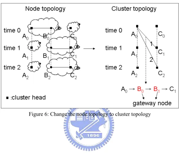
Figure 6: Change the node topology to cluster topology...6

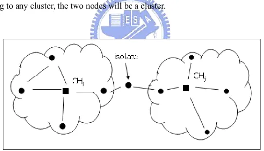
Figure 7: Becomes isolated because of the removing act ...10

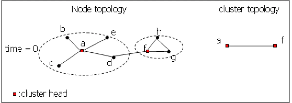
Figure 8: Links between clusters in space domain, case 1 ...11

Figure 9: Links between clusters in space domain, case 2 ...12

Figure 10: Links between clusters in time domain, case 1 and 2 ...13

Figure 11: Links between clusters in time domain, case 3 ...13

Figure 12: Links between clusters in time domain, case 4 ...14

Figure 13: Links between clusters in time domain, case 5 ...14

Figure 14: Links between clusters in time domain, case 6 ...15

Figure 15: Complexity of different t_ref ...22

Figure 16: Delivery delay of different t_ref...22

Figure 17: Diameter:250× node _number, time complexity...24

Figure 18: Diameter:250× node _number, delivery delay...24

Figure 19: Diameter:2500, time complexity...25

Figure 20: Diameter:2500, delivery delay ...26

Figure 21: Message size:10, delivery success rate in different value of α...28

Figure 22: Message size:15, delivery success rate in different value of α...28

Figure 23: Ratio ( node cluster # # ) in different value of α ...28

Figure 24: Message size:10, delivery success rate in different value of γ...29

Figure 25: Message size:15, delivery success rate in different value of γ...29

Figure 26: Ratio ( node cluster # # ) in different value of γ...30

Figure 27: Number of nodes is 50, delivery success rate. ...30

Figure 28: Number of nodes is 50, delivery delay. ...31

Figure 29: Number of nodes is 100, delivery success rate ...31

Figure 30: Number of nodes is 100, delivery delay...32

Figure 31: Time complexity...33

List of Equation

(

)

2 T N X = × Equation 1 ...16 T T n avg ref t total Y t ref i + × + − × =

∑

− = 2 1 _ 1 ) ( ) _ _ _ ( deg deg Equation 2 ...16

) ( ₂ 2 n N O Y X Z = = Equation 3...17 N deg N deg × = − × − + × = α α α ] 0 [ _ ] 1 [ _ _ 1 ) 1 ( ] [ _ i i i pri Node t accu load Node t pri Node Equation 4...18 ⎪ ⎪ ⎩ ⎪⎪ ⎨ ⎧ ∈ × + ∈ + =

∑

− = member node , # 1 head. cluster node , # 1 ] [ _ _{# 1} 0 member x x i i OutDeg OutDeg member member t load node ... Equation 5 ...19 0 ] 0 [ _ _ ] [ _ ) 1 ( ] 1 [ _ _ ] [ _ _ = + − × − = i i i i accu load Node t load Node t accu load Node t accui load Node γ ... Equation 6 ...20

List of Table

Table 1: Graph’s diameter :250× node _number, node’s average degree ...23

Table 2: Ratio of #cluster...23

Table 3: Diameter:250× node _number, the analysis of time complexity ...24

Table 4: Diameter:2500, the analysis of time complexity ...25

Table 5: Additional delay in different environments ...26

Chapter 1: Introduction

The conventional routing protocols applied to the wireless ad-hoc network

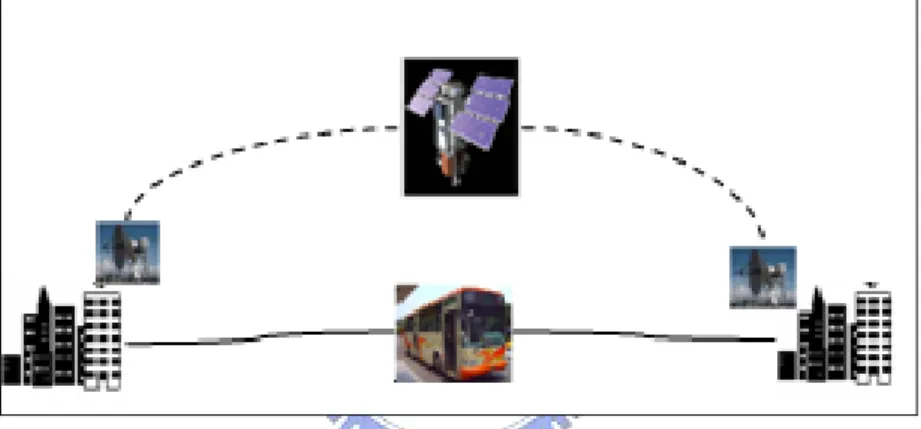
always assume that nodes are mostly connected with each other. But in some special environments, ex. Terrestrial mobile networks, as Figure 1, buses can be used to store

and forward messages, but the mobility of buses makes the network become intermittent connected; Exotic media networks, as in Figure 2, contain satellite

networks, long-distance wireless network, or underwater networks, hence we can predict this will result in intermittent connection, high delay, and broken cause of the

environment; Military Ad-Hoc Networks, routing in this kind of network may be in hostile environments where mobility, environmental factors, or intentional jamming

may cause for disconnection; Sensor network, these networks are frequently characterized by extremely limited end-node power, memory, and CPU capability. In

addition, they are envisioned to exist at tremendous scale, with possibly thousands or millions of nodes per network. Communication within these networks is often

scheduled to conserve power, and sets of nodes are frequently named only in aggregate. The challenges of routing in the network are high delivery delay,

intermittent connection, large queuing delay, and buffer limitations at intermediate nodes. This kind of network is the so-called delay tolerance network (DTN) [1][2].

Figure 1: Terrestrial mobile networks

Figure 2: Exotic media network

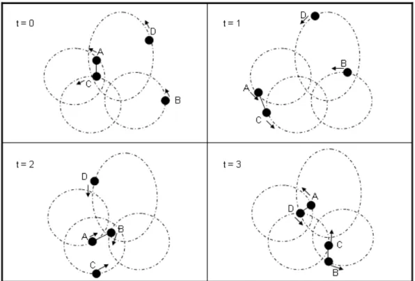
Although messages can be sent to the destination by storage and forwarding of relayed nodes, we cannot promise that messages will have the minimal delivery delay.

For example, Figure 3, messages from node A to node B are routed through node A at time=0, node C at time=0, node C at time=1, node C at time=2, node C at time=3,

finally node B at time=3. But the second path through node A to node B at time=2 has smaller delivery delay.

Figure 3: Can not promise that messages will have the minimal delivery delay

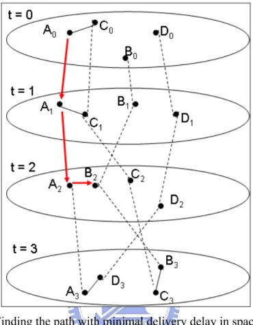
Hence, we use space and time information to generate graph with links in space

and time domain. And the links in the time domain are connections between the same nodes in different time intervals. For example, we transfer Figure 3 to Figure 4. In

Figure 4, the lines between nodes mean that the nodes are in the same transmission range in the same time interval. The dotted lines connect the same nodes in different

time intervals. The shortest path from node A to node B is A0 -> A1 -> A2 -> B2, so we

will adopt the second path in Figure 3 to send the message from node A to node B.

Routing in space and time can be applied to GPS (global positioning system); the information of dynamic position, time, speed, and schedule of the path to destination

can be known by GPS. The navigation center displays the trajectory of the vehicles’ mobility, and vehicles can also get the information needed from the navigation center,

for example, who data needed from other vehicles has to be relayed from whom. [3] proposes to find the path with minimal delivery delay with space and time

information. [4] also uses a knowledge oracle to obtain the connection between nodes.

Figure 4: Finding the path with minimal delivery delay in space and time

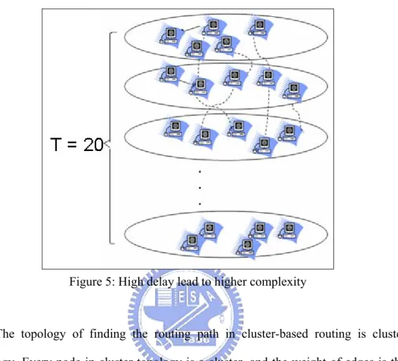
The complexity of applying the Dijkstra algorithm to find the routing path using

space and time information is where N is the number of nodes, T is total

time, and is the graph size. Hence, the complexity is proportional with the

number of nodes and the total time considered of finding the routing path. In DTN,

the high delay between nodes will lead to larger total time intervals needed by finding the routing path, so the complexity becomes large. For example,

2 ) (N×T

)

(

N

×

T

Figure 5 shows that

if the number of nodes is 50 and the total time intervals are 20, the complexity will be . Our purpose is to decrease the complexity of routing with space and time

information in DTN, we focus on reducing the topology by using cluster topology to get the routing path. We propose the cluster-based routing with space and time

2 ) 20 50 ( ×

information to group the nodes into clusters, thus the topology is reduced.

Figure 5: High delay lead to higher complexity

The topology of finding the routing path in cluster-based routing is cluster

topology. Every node in cluster topology is a cluster, and the weight of edges is the time cost by sending messages between two clusters, and the links between clusters

are formed by deploying the members of each cluster as the gateway node, like Figure 6, the links between clusters are A0 -> B0 -> B1 -> C1, and A0 -> B0 ->BB1 -> B2 -> C2.

B0B , B1 and B2 are gateway nodes. If we ignore the delay in the same time interval, we

can obtain that A₀C₁ =1, and A₀C₂ =2 in the cluster topology. Compared to the original topology, which uses all the nodes to find the routing path, cluster topology is

less complex. However, using cluster-based routing to decrease the complexity will lead to two problems. The first one is the additional space delay because messages

will be sent to cluster head first, but the space delay is much smaller compared to the total delivery delay in DTN, so it can be ignored. The second one is the heavier load

of cluster head, and we use load balance clustering by choosing nodes with lower loads to be cluster heads and gateway nodes to avoid congestion.

Chapter 2: Related Work

In terms of routing in DTN, we can divide it into two cases. The first one is the

deterministic case, which sends packets by predicting future connections. The second one is the stochastic case, which sends packets to any encountered node. We will

discuss the deterministic case and the stochastic case in the following two sections.

2.1 Deterministic case

In order to adapt the network with mobility, the space and time routing comes

into existence by using predictable mobility to find the routing path with minimal delivery delay[3]. This kind of algorithm involves links in time domain into graph,

and modifying Floyd-Warshall algorithm to find the routing path. The complexity is . In terms of predicting the path,

)

(_N3_{×T [4] mentions that a node’s mobility in DTN} can usually be predicted, and proposes using knowledge oracles to support the situations of nodes in the future. Exploiting the oracles derives five algorithms, and

the five algorithms individually use the oracle to predict the connection between nodes, the sending and receiving of buffer of nodes, and the flow in the network, and

then raise delivery success rate according to the oracles; [5] [6] assume that each node knows every node’s position at anytime completely, and builds the tree diagram to

search for the routing path. Therefore, it can build connections in wireless network and even in intermittent connected network.

2.2 Stochastic case

With “epidemic routing”, mentioned in [7][8], the source node broadcasts the messages continuously, and the node that receives the messages will also broadcast

the messages as the source node. The routing method also uses the timer mechanism to delete the messages to reduce the load of nodes. When messages are successfully

sent to the destination, “epidemic routing” uses a passive cure to remove the successfully relayed messages from the buffer of nodes which help relay the

messages.

“PROPHET”[9] defines the transmission probability between nodes and updates

the probability when nodes encounter each other. Using the probability to decide whether the packet needs to be relayed by encountered node or not can reduce the

load of network efficiently and can obtain acceptable delivery success rate.

“Message Ferrying” [10] [11] [12] [13] [14] [15] [16] uses gateway nodes

(which gather data at each area and exchange data with ferry nodes) and ferry nodes (which move around in every area and exchange data with gateway nodes) to transmit

data in different areas. [12] divides the decision of gateway node used to contact with ferry nodes into three cases: stochastic, proportional, and the node close to the source

node. The ways to transmit data between ferry nodes and gateway nodes are also divided into three types, outgoing first, incoming first, and round robin. It exploits

Chapter 3: Cluster-based Routing with Space and

Time Information

In order to find the routing path, we find the cluster which involves the source

node and the cluster which involves the destination node. Apply the Dijkstra algorithm with cluster topology to find the routing path between the two clusters.

Then, use the routing path between clusters to find the mapped path between nodes to get the complete path between the source node and the destination node. The routing

method is divided into two steps.

(1) Construct cluster: Exploit greedy method to find the node which covers the most

nodes to be the cluster head, and turn the covered nodes into a cluster.

(2) Links between clusters: Exploit the members of clusters to connect to other

clusters to form the links between clusters.

Detailed discussions are in the following two sections.

3.1 Construct cluster

We divide the cluster construction into two parts. One is that cluster will have two-hop member at most. The other is that connected nodes will be a cluster. Detail

discussion is as following two sections.

3.1.1 Two-hop cluster

Exploit greedy method to find the node which covers the most nodes to be the

cluster head, and the covered nodes become a cluster. Then, remove the nodes in the cluster from the graph. Keep finding the cluster head until all nodes are removed from

nodes. The isolated nodes may be unconnected with other nodes or originally connected with other nodes, but will become isolated because of the removing act, as

in Figure 7. So the isolated node will be checked to see if it is connected with any other cluster or not. If the isolate node is connected with another cluster, it will

become the member of a connected cluster. Otherwise, the isolated node will be formed to be a cluster itself because of the necessity of all nodes being deployed to

find the routing path. If the isolate node is not formed to be a cluster, it will not be considered in the cluster topology, and this will lead to the absence of some routing

paths. Therefore, the isolated node will also be formed to be a cluster. Hence, the members are at most two hops away from the cluster head. The members that are

three hops away will not exist because if there are two connected nodes which do not belong to any cluster, the two nodes will be a cluster.

Figure 7: Becomes isolated because of the removing act

3.1.2 Connected cluster

Exploit greedy method to find the node which covers the most nodes to be the

cluster head. Then make all connected node be involved into the cluster. Remove the nodes in the cluster from graph. Keep finding the cluster head until all nodes are

3.2 Links between clusters

Deploy the nodes of each cluster to connect to other clusters. Links in the space

domain are only in the same time interval, and links in the time domain are deploying clusters of nodes to check if any cluster can be connected in other time intervals, and

the number of time intervals being checked is t_ref. Here we set the value of t_ref to be 2 to discuss links in space and time in the following two sections.

3.2.1 Links between clusters in space domain

Deploy the members of each cluster to connect to other clusters in the same time interval. There are two cases. The first one is that if a member’s neighbor is a cluster

head, the two clusters are connected, as in Figure 8, node d is cluster a’s member, and node f is node d’s neighbor, so clusters a and f are connected by node d. The second

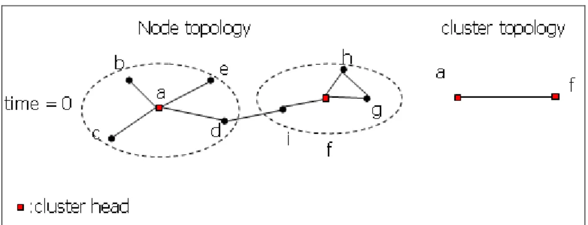
one is that if the member’s neighbor belongs to other clusters, the two clusters are connected, like Figure 9, node d is cluster a’s member, and node d’s neighbor, node i,

is cluster f’s member, so clusters a and f are connected by node d and node i.

Figure 9: Links between clusters in space domain, case 2

3.2.2 Links between clusters in time domain

Connect the clusters in time domain to make a message that can not only route in space but also in time. Six situations will be discussed as following.

The first two cases are deploying cluster head to build the links, and the first one is that the node is a cluster head now and is also a cluster head in the next time

interval. The second one is that the node is a cluster head now but is not a cluster head in the next time interval. In the first case, we can directly connect two nodes and set

the weight to be the time as an interval. In the second case, we need to check which cluster the node belongs to in order to connect them. For example, in Figure 10, the

first case is that node f is cluster head at time=0 and time=1, directly connect the two clusters, cluster f at time=0 and cluster f at time=1, and the weight is 1. The second

case is that node a is a cluster head at time=0, but it’s not a cluster head at time=1, connect cluster a at time=0 to cluster c at time=1 which contains node a.

Figure 10: Links between clusters in time domain, case 1 and 2

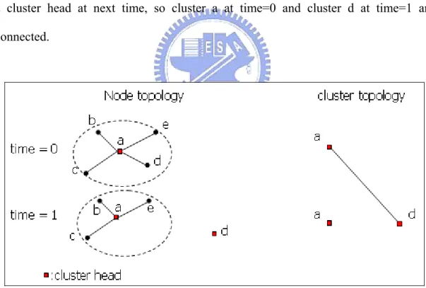
The third case is that if a member is a cluster head in the next time interval, the

two clusters are connected, as in Figure 11, node d belongs to cluster a, and node d is a cluster head at next time, so cluster a at time=0 and cluster d at time=1 are

connected.

Figure 11: Links between clusters in time domain, case 3

The fourth case is that if a member belongs to another cluster in the next time

interval, the two clusters are connected, as in Figure 12, node d belongs to cluster a at time=0 and belongs to cluster f at time=1, so cluster a at time=0 and cluster f at

time=1 are connected by node d.

Figure 12: Links between clusters in time domain, case 4

The fifth case is that if a member’s neighbor is a cluster head in the next time

interval, the two clusters are connected, as in Figure 13, node d belongs to cluster a at time=0 and node d’s neighbor, node f, is a cluster head at time=1, so cluster a at

time=0 and cluster f at time=1 are connected by node d.

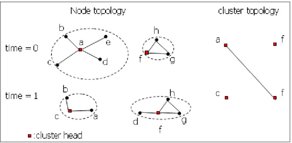
next time interval, the two clusters are connected, as in Figure 14, node d belongs to cluster a at time=0, and the neighbor of node d, node h, belongs to cluster f at time=1,

so cluster a at time=0 and cluster f at time=1 are connected by node d and node h.

Chapter 4: Complexity analysis

The graph size without clustering is the number of nodes plus the total time intervals, #node×T(T: total time intervals), and the complexity of finding the shortest path by Dijkstra algorithm is , so the complexity of finding the

routing path with space and time without clustering is X, as in 2 ) (totalnodes Equation 1.

(

2 T N X = ×

)

Equation 1

The meanings of the mathematical symbols in Equation 1 are as follows:

1. N: The number of nodes 2. T: Total time intervals

3. N×T : Graph size in non-clustering

The total complexity of finding the routing path with cluster-based routing is Y, as in Equation 2. T T n avg ref t total Y t ref i + × + − × =

∑

− = 2 1 _ 1 ) ( ) _ _ _

( deg deg Equation 2

The meanings of the mathematical symbols in Equation 2 are as follows: 1. n : Number of clusters

2. T : Total time intervals

3. total_deg : Sum of every node’s degree

4. avg_deg :

T total_deg

5. n×T : Graph size in clustering

ref t

total_deg× _ comes from the fact that nodes will check all of their

neighbors in the time intervals, t_ref. And

∑

means that when a node is

−1 _ _ ref t avg deg

at the time=t, the node does not need to check the time interval, t+t_ref −1 if the time is larger than T. The complexity of applying Dijkstra to find the

routing path is , where T is result from the destination node belongs to

different clusters in different time intervals. 1 _ − +t ref t T T n× ₎2+ (

The analysis of the complexity in the two methods of non-clustering and clustering is as Equation 3. ) ( ₂ 2 n N O Y X Z = = Equation 3

The cluster topology is smaller than node topology because n< , so Z will be N

larger than 1. It means that topology with clustering will reduce the complexity of

Chapter 5: Load Balance Clustering Method

Cluster-based routing will lead to a heavy load of the cluster head, so we propose

load balance clustering to avoid congestion of nodes with heavy load. Load balance clustering is divided into two steps: choosing nodes with lower load to be cluster

heads and choosing nodes with lower load gateway nodes. We discuss the two aspects as following.

5.1 Choosing a proper cluster head

Change the decision of choosing cluster head from only caring about the node’s degree to also take the past load into consideration. The purpose here is to choose the

node with a higher degree and lower load. Higher degree will lead to less number of clusters because chosen nodes will cover more nodes, and lower load will decrease

the load of cluster head. Therefore, we use a priority function to choose the node with a higher degree and lower load to be cluster head. The priority of being chosen to be

the cluster head is shown in Equation 4. The higher the priority, the higher the degree and the lower the load in the past, hence, it can decrease congestion in the

network. N deg N deg × = − × − + × = α α α ] 0 [ _ ] 1 [ _ _ 1 ) 1 ( ] [ _ i i i pri Node t accu load Node t pri Node Equation 4

The meanings of the mathematical symbols in Equation 4 are as followes: 1．α : Ratio of degree and load

3．N : The number of nodess

The value of α affects the proportion of degree and load. If α is too high,

nodes may congest easily, and it will lead to a lower delivery success rate because

messages will be delayed in heavy load nodes and miss the possible routing path. If α is too low, it will lead to more clusters because the range covered by a cluster

becomes small. We discuss the value in our simulation. And the load’s definition is as Equation 5, ⎪ ⎪ ⎩ ⎪⎪ ⎨ ⎧ ∈ × + ∈ + =

∑

− = member node , # 1 head. cluster node , # 1 ] [ _ _{# 1} 0 member x x i i OutDeg OutDeg member member t load node Equation 5

The meanings of the mathematical symbols in Equation 5 are as follows: 1．#member ：The number of members in the cluster

2．OutDeg ：The degree of nodes excluding the members of the self cluster

Because messages will be sent to the cluster head first, the load of cluster head involves the member of self cluster and itself. The load of member takes how many

nodes will transmit messages from itself into consideration. Therefore, if the out degree ( the degree of nodes excluding the member of self cluster ) of the node is

large, the probability of helping relay data will also increase, and the load becomes high. And the load of nodes will be accumulated and also will decay with time, the

0 ] 0 [ _ _ ] [ _ ) 1 ( ] 1 [ _ _ ] [ _ _ = + − × − = i i i i accu load Node t load Node t accu load Node t accui load Node γ Equation 6

The meanings of the mathematical symbols in Equation 6 are as follows: γ ：Decay ratio

The value of γ will effect decay of the load, if γ is high, it means messages

will be sent quickly and load will decay right away. And we will discuss the value of γ in our simulation.

5.2 Choosing a proper gateway node

The main purpose is to choose a node with a lower load to help relay in order to avoid congestion. We assume that if a node is often chosen to be gateway node, it will

have a higher load. Therefore, if the node is often chosen to be a gateway node, it is not proper to be the gateway node between clusters. It means that if two more nodes

can be used to connect the two clusters, we choose the node which is seldom chosen to help relay to be the gateway node between two clusters in order to decrease the

Chapter 6: Simulation

Because of the difficulty of developing a delay tolerance network, the experiments are made through simulation, and deploy ns2 network simulation

environment to generate patterns of the connections between nodes. The mobility model uses a random method. The sparse nodes and movement with high speed are

used to simulate an intermittent connected and rapid varying network.

The DTN simulator is an event-driven simulator written in C and links are

attached to nodes by patterns with finite propagation delay and finite bandwidth. Its main purpose is to simulate DTN-like store and forwarding of messages over long

period of time.

“Cluster-based routing space and time with space and time”, additional space

delay, and “Load balance clustering” are simulated in the following.

6.1 Cluster-based routing with space and time information

We use simulation to compare the performance of the algorithms with two-hop

clustering, connected clustering and without clustering in different environments and discuss with the three merits, time complexity, average delivery delay, and path not

found. In order to observe the difference of delivery delay obviously, the weight of space link is set to be 0.1. Before the discussion of different algorithms, we need to

know the influence of the parameter, t_ref, which is the time interval checked when exploit members to find the routing path between clusters in our simulator. The

influence of t_ref and the performance of cluster-based routing are discussed in the following two sections.

6.1.1 Influence of t_ref

Figure 15 shows that the complexity will increase with the value of t_ref

increasing. It’s because the more time intervals are checked, the more edges be found in the cluster topology. Figure 16 shows that the delivery delay is almost the same in

different value of t_ref except for the value of t_ref is 1. If the value of t_ref is 1, this means that members only find the neighbors in space with a lack of time, so the

delivery delay will become higher. Hence, we use 3 to be the value of t_ref.

0 20 40 60 80 100 120 10 20 30 40 50 60 70 80 90 100 node number co st t im e( m s) t_ref=1 t_ref=2 t_ref=5 t_ref=10 t_ref=15

Figure 15: Complexity of different t_ref

0 0.5 1 1.5 2 2.5 3 3.5 4 10 20 30 40 50 60 70 80 90 100 node number de live ry delay (s) t_ref=1 t_ref=2 t_ref=5 t_ref=10 t_ref=15

6.1.2 Performance of cluster-based routing

The simulation is performed with two scenarios, static node density and static

graph diameter. In the scenario of the static node density, the graph’s diameter is set to

be 250× node _number, and the node degree is like Table 1 which shows that every node has about 4 to 6 links. The number of clusters is 20% of the number of

nodes in two-hop clustering and 10% of the number of nodes in connected clustering as Table 2. Therefore, the time complexity of two-hop clustering and connected

clustering should be (0.2)2 = 4% and (0.1)2 = 1% of non-clustering’s theoretically. Figure 17 and Table 3 show that the complexity of two-hop clustering and connected

clustering are individually almost 4% and 1% of non-clustering’s and the result matches to the theoretical value. Also, the delivery delay of clustering is increased

slightly as Figure 18. And all paths can be found in the scenario by using the three algorithms.

#node 10 20 30 40 50 60 70 80 90 100

Degree 4.6 4.26 4.75 5.62 5.96 6.08 6.08 6.27 6.73 6.35

Table 1: Graph’s diameter :250× node _number, node’s average degree

Algo#node 10 20 30 40 50 60 70 80 90 100

two-hop 2.1 4.85 7.35 9.15 11.4 13.15 15.4 18.1 20.45 22.25 Connect 1.75 2.85 4.15 4.55 6.1 6.3 7.2 9 10.3 10.55

0 500 1000 1500 2000 10 20 30 40 50 60 70 80 90 100 node number co st tim e( m s) ori two-hop connect

Figure 17: Diameter:250× node _number, time complexity

Algo#node 10 20 30 40 50 60 70 80 90 100 Original 0 10 46 108 202 354 586 858 1170 1712 Two-hop 0 1 3 4 6 19 28 41 53 81 Ratio 0 10.0 15.3 27.0 33.7 18.6 20.9 20.9 22.1 21.1 Connect 0 1 2 2 2 4 4 6 6 9 Ratio 0 10.0 23.0 54.0 101.0 88.5 83.7 107.3 117.0 114.1

Table 3: Diameter:250× node _number, the analysis of time complexity

1.00 2.00 3.00 4.00 5.00 6.00 10 20 30 40 50 60 70 80 90 100 node number de live ry de la y( s) ori two-hop connect

In the scenario of the static graph diameter, the graph diameter is set to be 2500. Time complexity, average delivery delay, and path not found are discussed. Figure 19

shows that the complexity of clustering is smaller than the non-clustering’s and the ratio is as shown in Table 4. The delivery delay of clustering is increased slightly as in

Figure 20. 0 500 1000 1500 2000 10 20 30 40 50 60 70 80 90 100 node number co st ti m e( ms 0 ori two-hop connect

Figure 19: Diameter:2500, time complexity

Algo #node 10 20 30 40 50 60 70 80 90 100 Original 0 10 16 38 122 228 454 764 1154 1730 Two-hop 0 1 4 6 18 20 34 50 56 90 Ratio 0.00 3.33 4.00 6.33 6.78 11.40 13.35 15.28 20.61 19.22 Connect 0 1 4 4 12 14 14 14 14 16 Ratio 0.00 5.00 4.00 9.50 10.17 16.29 32.43 54.57 82.43 108.13 Table 4: Diameter:2500, the analysis of time complexity

4 6 8 10 12 14 10 20 30 40 50 60 70 80 90 100 node number de liv er y de la y( s0 ori two-hop connect

Figure 20: Diameter:2500, delivery delay

6.2 Additional delay

The graph diameter is 250× node _number for the same node density, data rate is 54 M bit as the max data rate in 802.11a and packet size is 2304 octets as the maximum packet size in 802.11. Table 5 shows that The ratio

(_complexitycomplexity_ofof_originalcluster ) is ranged from 0.012% to 0.024%, the additional space

delay results from cluster-based routing can be ignored because the total delivery delay is larger than it.

Algo node 10 20 30 40 50 60 70 80 90 100 Cluster 1.7789 2.6933 3.2844 2.9249 3.2552 3.1383 2.9036 3.2452 3.7254 2.4778 Original 1.7786 2.6929 3.2840 2.9244 3.2547 3.1377 2.9031 3.2446 3.7247 2.4772 Ratio 0.019% 0.012% 0.013% 0.016% 0.016% 0.017% 0.018% 0.018% 0.020% 0.024% Table 5: Additional delay in different environments

balancing (cluster), improving choosing the cluster head (imp_CH), improving choosing the gateway node (imp_gate), and improving both (combine) are deployed

in the DTN-simulator. And when node wants to send a message, it will send a request and then send the message until it receives a reply. The request size is 1Kb, reply

message size is 1Kb, and message size is 10Kb. The queue size is infinite here. The data rate is 1Mb and the connection in every time interval will exist for half an

interval. We define delivery success rate of a routing algorithm as the ratio of the number of messages that are successfully delivered to the total number of messages

that are forwarded. The discussion of the simulation is divided into three parts as the influence of the parameters used in the load balance clustering, the improvement of

delivery success rate, and the influence of the cluster head’s rise by load balance clustering.

6.3.1 Influence of the parameters in load balance clustering

The simulation here will fix the value of α and γ individually to see the

influences of the two values. The graph diameter is250× node _number , the number of nodes is 50, messages are sent from every node to every other node, and γ is fixed to be 0.5 to see the influence of α with different loads. Figure 23 shows that the influence of α to the ratio of clusters is below 5%. Figure 21 and Figure 22

show that if α is 1, the delivery success rate is the lowest at different message sizes. This is because the load is not taken into consideration when choosing the cluster

93.00% 94.00% 95.00% 96.00% 97.00% 98.00% 99.00% 100.00% 101.00% 0.1 0.2 0.3 0.4 0.5 0.6 0.7 0.8 0.9 1 α delivery succes s rate

Figure 21: Message size:10, delivery success rate in different value of α

75.00% 80.00% 85.00% 90.00% 95.00% 0.1 0.2 0.3 0.4 0.5 0.6 0.7 0.8 0.9 1 α

de

liv

er

y

su

cces

s r

ate

Figure 22: Message size:15, delivery success rate in different value of α

0.00% 10.00% 20.00% 30.00% 40.00% 0.1 0.2 0.3 0.4 0.5 0.6 0.7 0.8 0.9 1 α rati o of #C H Figure 23: Ratio ( node cluster # # ) in different value of α

Fix α to be 0.7 to see the influence of γ with different loads (The number of message every node send to any other node). Figure 26 shows that the influence of γ

to the ratio of clusters is below 5%. Figure 24 and Figure 25 show that if γ is 1, the performance is the worst with different loads. This is because when γ is 1, just

consider the load at a previous time instead of the load in the past while choosing the cluster head. Therefore, we set γ to be 0.5 to be performed in our DTN simulator.

94.00% 95.00% 96.00% 97.00% 98.00% 99.00% 100.00% 101.00% 0.1 0.2 0.3 0.4 0.5 0.6 0.7 0.8 0.9 1 γ del iv er y success rat e

Figure 24: Message size:10, delivery success rate in different value of γ

10.00% 15.00% 20.00% 25.00% 30.00% 0.1 0.2 0.3 0.4 0.5 0.6 0.7 0.8 0.9 1 γ rat io of #C H Figure 26: Ratio ( node cluster # # ) in different value of γ

6.3.2 Improvement of delivery success rate

We observe the improvement with different loads in the scenario of the static

node density (graph’s diameter is 250* node _number) and static number of nodes.

When the number of nodes is 50 and messages are sent from every node to every

other node, Figure 27 shows that improving choosing cluster head and gateway node can improve the delivery success rate about 5% to 10 %. Also, the delivery delay is

increased slightly as shown in Figure 28.

50.00% 60.00% 70.00% 80.00% 90.00% 100.00% 10 12 14 16 18 20 message size delivery s uc ce ss rate _cluster imp_gate imp_CH combine

8 8.5 9 9.5 10 10.5 11 11.5 10 12 14 16 18 20 message size delivery delay(s) cluster imp_gate imp_CH combine

Figure 28: Number of nodes is 50, delivery delay.

When the number of nodes is 100 and messages are sent from half nodes to other

half nodes, Figure 29 shows that improving the choosing of the cluster head and gateway node can improve the delivery success rate by about 5% to 10 %. Also, the

delivery delay is increased slightly as shown in Figure 30.

40.00% 50.00% 60.00% 70.00% 80.00% 90.00% 100.00% 10 12 14 16 18 20 message size deliver r ate cluster imp_gate imp_CH combine

9 9.5 10 10.5 11 11.5 10 12 14 16 18 20 message size delivery delay(s) cluster imp_gate imp_CH combine

Figure 30: Number of nodes is 100, delivery delay

6.3.3 Influence of the number of clusters after improving cluster choosing

We observe the influence in the scenario of the static node density ( the graph’s

diameter is 250* node _number ). Improving cluster choosing will lead to the

increase of clusters as Table 6, so the time complexity will also increase. Figure 31

shows that the influence is slight, and the result matches to the theoretical value as Figure 32 counted by the number of clusters and the number of

nodes . 2 ) (n×T 2 ) (N×T Algo#node 10 20 30 40 50 60 70 80 90 100 CH 2.1 4.9 7.4 9.2 11.4 13.2 15.4 18.1 20.5 22.3 Imp_CH 2.3 5.0 8.0 10.0 12.9 14.8 18.7 21.5 24.0 26.3 Table 6: Average number of clusters in each time interval

0 200 400 600 800 1000 1200 1400 1600 1800 10 20 30 40 50 60 70 80 90 100 node number cost time(ms) cluster imp cluster original

Figure 31: Time complexity

0 2000 4000 6000 8000 10000 12000 10 20 30 40 50 60 70 80 90 100 node number complexity cluster imp cluster original

Chapter 7: Conclusion

In this thesis, because messages delivered by storing and forwarding can’t have minimal delay, we adopt the method of predictable mobility to find the routing path.

We focus on reducing the topology by using cluster-based routing. Using the cluster topology will reduce the graph needed by finding the routing path, and this will lead

to lower complexity. The first one of the extended problems is the additional space delay because messages will be sent to cluster head first, but the additional space

delay is much smaller compared to the total delivery delay. And the second one of the extended problems is the heavy load of cluster heads. It is improved by load balance

clustering, and simulation shows that load balance clustering can improve the delivery success rate.

Reference

[1] Delay-tolerant networking research group. http://dtnrg.org

[2] Kevin Fall, “A Delay-Tolerant Network Architecture for Challenged Internets”,

in Proceedings of ACM SIGCOMM’03, August 2003.

[3] Shashidhar Merugu, Mostafa Ammar, Ellen Zegura, “Routing in Space and Time

in Networks with Predictable Mobility”, Technical Report GIT-CC-04-7, Georgia Institute of Technology, 2004.

[4] Sushant Jain, Mostafa Ammar, Ellen Zegura, “Routing in a Delay Tolerant Network”, in Proceedings of ACM SIGCOMM’04, August 2004.

[5] Radu Handorean, Christopher Gill and Gruia-Catalin Roman, “Accommodating Transient Connectivity in Ad Hoc and Mobile Settings”, Lecture Notes in

Computer Science, 2004.

[6] A. Ferreira, “Building a reference combinatorial model for MANETs”, IEEE

Network, October 2004.

[7] A. Vahdat and D. Becker, “Epidemic routing for partially connected ad hoc

networks”, Tech Report CS-2000-06, Duke University, July 2000.

[8] T. Small and Z. J. Haas, “The Shared Wireless Infostation Model - A New Ad

Hoc Networking Paradigm (or Where there is a Whale, there is a Way)”, in Proceedings of Mobihoc 2003, June 2003.

[9] Anders Lindgren, Avri Doria, and Olov Schelén, “ Probabilistic routing in intermittently connected networks”, ACM SIGMOBILE Mobile Computing and

[10] W. Zhao , M. Ammar , E. Zegura, “A Message Ferrying Approach for Data Delivery in Sparse Mobile Ad Hoc Networks”, in Proceedings of the 5th ACM

international symposium on Mobile ad hoc networking and computing, May 2004.

[11] S. Dolev, S. Gilbert, N. Lynch, E. Schiller, A. Shvartsman, and J. L. Welch, “Virtual Mobile Nodes for Mobile Ad Hoc Networks”, in Proceedings of 18th

International Symposium on Distributed Computing (DISC), 2004.

[12] Yang Chen, Wenrui Zhao, Mostafa Ammar and Ellen Zegura, “Hybrid Routing

in Clustered DTNs with Message Ferrying”, in Proceedings of ACM SIGMOBILE Mobile Opportunistic Networking (MobiOpp), 2007.

[13] D. Nain, N. Petigara, and H. Balakrishnan, “Integrated Routing and Storage for Messaging Applications in Mobile Ad Hoc Networks”, in Proceedings of WiOpt,

March 2003.

[14] F. Tchakountio and R. Ramanathan, “Tracking highly mobile endpoints”, In

Proceedings of ACM Workshop on Wireless Mobile Multimedia (WoWMoM), July 2001.

[15] R. C. Shah, S. Roy, S. Jain, and W. Brunette, “Data MULEs: Modeling a Three-tier Architecture for Sparse Sensor Networks”, in Proceedings of IEEE

Workshop on Sensor Network Protocols and Applications (SNPA), May 2003.

[16] C. Shen, G. Borkar, S. Rajagopalan, and C. Jaikaeo, “Interrogation-based relay

routing for ad hoc satellite networks”, in Proceedings of IEEE Globecom, November 2002.