實現感應電動車最大加速性能與最高效率之控制設計與切換策略

國立交通大學

電機與控制工程學系

碩士論文

實現感應電動車最大加速性能與最高效率之

控制設計與切換策略

研 究 生：郭志瀚

指導教授：徐保羅 博士

中 華 民 國 一 百 零 一 年 七 月

The Control Design and Switching Strategy for Maximizing Acceleration

and Efficiency of the Induction Machine on Electric Vehicles

研 究 生：郭志瀚

Student : Chih-Han, Kuo

指導教授：徐保羅 博士

Advisor : Dr. Pau-Lo Hsu

國立交通大學

電機與控制工程學系

碩士論文

A Thesis

Submitted to Institute of Electrical Control Engineering College of Electrical and Computer Engineering

National Chiao Tung University in Partial Fulfillment of the Requirements

for the Degree of Master in

Electrical Control Engineering July 2012

Hsinchu, Taiwan, Republic of China

中 華 民 國 一 百 零 一 年 七 月

實現感應電動車最大加速性能與最高效率之控制設計與切換策略

The Control Design and Switching Strategy for Maximizing Acceleration and

Efficiency of the Induction Machine on Electric Vehicles

實現感應電動車最大加速性能與最高效率之控制設計與切換策略

研究生: 郭志瀚 指導教授: 徐保羅 博士

國立交通大學電控工程研究所

中文摘要

隨著近年來電動車技術以提高效率與扭力性能為目標發展，採用永磁馬達的 高功率密度與高扭力密度的表現固然較佳，但感應馬達低成本、高耐用度與廣域 操作速度的特性，為永磁馬達所不及之優勢；且在輕型電動車輛之應用上，更能 突顯小功率感應馬達在高過負載能力的優勢。但欲達成感應馬達車用動力之高扭 力與高效率的訴求，在控制技術上仍屬一大挑戰。因此，本研究致力於發展感應 馬達之精密伺服控制，成功以德州儀器TMS320F28335 DSP晶片實現電動車兼具 最大扭力與最高效率之自動切換控制策略。 在間接向量控制的實現中，為了達成磁場與扭力的動態控制，需進行感應馬 達同步電氣角的估測，其計算乃建立在轉子時間常數(rotor time constant)的基礎 上，此參數量測準確與否將影響控制的性能。有鑑於傳統轉子時間常數的量測方 式實現困難，本研究發展以加速度為判斷依據的鑑別方法，不僅量測結果具有高 準確度，且可直接在車輛上量測而更加容易實現；此外，為了達到單位電流最大 扭力(maximum torque per amperage, MTPA)的控制特性，通常是將磁場電流 (flux-producing current)與扭力電流(torque-producing current)設置於相同大小，但 此方法在電動車的應用上造成了嚴重的磁飽和現象，使扭力輸出不如預期。本研 究建立一套實驗標準程序，建立磁場操作電流與車輛加速度的關係，並選用額定 激磁操作達成車輛的最大加速性能。 雖然MTPA擁有最大的加速表現，但在等速操作時效率較差。普遍的做法是 在車輛加速過程後，藉由調整磁場電流達成效率的提升，但在電流切換時將造成 車輛駕駛不平順的現象。本研究提出一套新式的切換控制策略，所定義之滑差因 素(slip factor)將根據駕駛情況自動調整，在車輛低速時保有最大加速性能、在高 速的情況則有最高的效率輸出，且實驗結果證明此方法在切換過程中具有更平順 的電流操作；相較將磁場電流與扭力電流設為相同的方法，本控制策略在加速性、 效率與車輛尾速部分可分別改善67%、273.6%與111.8%。因此，本研究成功實現 了更適合電動車控制、且兼具高扭力效能及低耗電效率的感應馬達控制策略。

The Control Design and Switching Strategy for Maximizing

Acceleration and Efficiency of the Induction Machine on Electric

Vehicles

Student: Chih-Han, Kuo Advisor: Dr. Pau-Lo, Hsu

Institute of Electrical Control Engineering National Chiao Tung University

Abstract

As the environmental crises become more significant, electric vehicles have drawn more attentions and have been rapidly developed in recent years. Even though permenant magnetic motors (PM) are usually preferred due to their inherent characteritics of high torque and power density, induction motors (IM) behave better on the aspects of cost, reliability, and with a wider operational speed range. Particularly, IMs dominate PMs with higher overload capability on applications of low-powered electric vehicle. However, control techniques of IMs are still chanllenging to meet high-torque and high-efficiency vehicle performance. Therefore, this study is dedicated to developing a DSP-based precise servo control with maximizing torque and efficiency for the IM implemented on electric vehicles, and the developed automatic control strategy is successfully implemented on the TMS320F28335 DSP microcontroller.

The indirect vector control is commonly exploited for high performance servo control of the IM. To achieve control of the flux and torque, precise synchronous angle estimation based on the rotor time constant is crucial for stator current decoupling, and thus control performance is highly dependent on the accuracy of parameters. Due to the fact that conventional identification approaches are suffered from difficulty of implementation, an acceleration-based identification process which can be directly performed on the vehicle with satisfactory accuracy is developed in this thesis. In addition, the maximum torque per amperage (MTPA) operation is considerably important to provide desirable acceleration of the vehicle. It has been already recognized that by dividing the stator current equally into the flux-producing component and the torque-producing component, the MTPA can be thus obtained.

Nevertheless, such arrangement causes severe flux saturation and the desirable operation is usually lost. In this Thesis, a standard experimental process is developed to find proper setting of the flux-producing current so that the maximum acceleration can be fulfilled.

Despite of the maximum acceleration performance of the electric vehicle obtained by the MTPA operation, its operating efficiency is still comparatively low. In general, the efficiency can be improved by adjusting the flux-producing current. A novel switching control strategy where the defined slip factor can be automatically adjusted according to driving conditions is developed for achieving both the maximum acceleration and the highest efficiency, and experimental results show that it is more suitable to traction control of the electric vehicle because of its smooth operating performance. It has been also verified that all the acceleration, efficiency coefficient, and final vehicle speed can be improved by 67%, 273.6%, and 111.8%, respectively, when the system is fed by the maximum stator current compared with those of the conventional control approach by applying equal d-q current command.

Keywords: electric vehicle, induction motor, maximum torque per amperage, efficiency, rotor time constant identification, slip factor.

Acknowledgement

首先，我要由衷地感謝指導教授徐保羅老師在我這兩年研究生活的耐心指導 與建議，不論在研究或為人處事上培養我嚴謹的邏輯、正確的態度與問題解決的 能力，皆使我獲益良多，並順利地完成碩士學位。此外，感謝口試委員陳鴻祺老 師與葉賜旭老師對於本論文寶貴的建議與指正，使本論文更加完善。 感謝在實驗室裡陪伴在我身邊的學長、同學與學弟們：博士班賴建良學長、 黃煒生學長、謝鎮州學長與碩士班廖子期學長、葉釗甫學長、蔡政宏學長、林軒 正學長、黃思翰學長平時給我的指導與幫助；信佑、振文、誌緯、晟傑、琮昇在 學業上的討論與指教，以及一同度過研究所的時光，不論是研究上的切磋砥礪或 生活上的經驗分享，都是我碩士班生活不可或缺的美好回憶；另外，也非常感謝 實驗室助理慧霖，總是熱心地協助我們辦理各項事務，讓我們得以心無旁騖地進 行研究。在此特別感謝振文與誌緯，在研究與實驗上大力地幫忙，獻上我最誠摯 的感謝。 最後，我要感謝關心我的父母、妹妹以及女友題帆，長久以來在生活上的陪 伴與支持，讓我在遭遇挫折與難關時能更有信心與動力去克服，而得以完成碩士 學位。再次感謝求學歷程中所有幫助我、支持我與鼓勵我的師長與朋友，願將此 喜悅與榮耀與你們一同分享。

Contents

Abstract (Chinese) ... I Abstract (English) ... III Acknowledgement ... V Contents ... VI List of Figures ... VIII List of Tables ... XIII

Chapter 1 ... 1

1.1 Motivation and Purposes... 1

1.2 Problem Statements ... 4

1.3 Proposed Approaches ... 5

1.4 Organization of the Thesis ... 6

Chapter 2 ... 7

2.1 Transformation of Reference Frame ... 7

2.2 Dynamic Charactersitics of an Induction Machine ... 8

2.3 Indirect Vector Control ... 12

2.3.1 Principles of indirect vector control ... 12

2.3.2 Implementation of indirect vector control ... 13

2.3.3 Dynamic model of an indirect vector-controlled induction motor ... 15

2.4 Operation Region of an Induction Machine... 17

2.4.1 Voltage and current constraints on induction machine control ... 17

2.4.2 Capability curve of an induction machine ... 20

2.5 System Structure ... 21

2.5.1 Mechanical layout of the electric vehicle ... 21

2.5.2 Control program of the system ... 27

Chapter 3 ... 40

3.1 Identification Process of the Rotor Time Constant ... 40

3.1.2 Identification of the rotor time constant ... 43

3.2 Maximum Torque per Amperage Control ... 47

3.2.1 Approach of the equal d-q current command ... 47

3.2.2 Approach of the rated flux excitation ... 49

3.2.3 Experimental verification of the MTPA ... 55

3.3 The Highest Efficiency Operation ... 56

3.4 Summary ... 59

Chapter 4 Design of the Optimal Switching Mechanism ... 61

4.1 Slip Factor Adjustment (γ-Adjustment) ... 61

4.2 Comparison between the γ-Adjustment and the ids*-Adjustment... 66

4.3 Switching Strategy for Both the MTPA and the HE Operation ... 70

4.3.1 Design of the switching strategy ... 70

4.3.2 Experimental verification of the designed strategy ... 75

4.4 Summary ... 83

Chapter 5 Conclusion ... 85

List of Figures

Fig. 1-1 Current circumstances of electric machine selections for electric vehicles ... 2

Fig. 1-2 Illustration of research in this Thesis ... 3

Fig. 2-1 Relationship between reference frames ... 7

Fig. 2-2 Three-phase axis of the stator and rotor ... 9

Fig. 2-3 Equivalent circuit of the squirrel-cage induction motor... 12

Fig. 2-4 Illustration of stator current decoupling ... 14

Fig. 2-5 Block diagram of indirect vector control ... 14

Fig. 2-6 Dynamic model of the indirect vector-controlled induction motor ... 16

Fig. 2-7 Voltage constraint ellipses at different operation speed ... 18

Fig. 2-8 Circle of current constraint ... 18

Fig. 2-9 Parabolic curves of torque ... 19

Fig. 2-10 Possible operation points considering both voltage and current constraint ... 19

Fig. 2-11 Locus of voltage ellipse, current circle, and torque in different operation regions ... 20

Fig. 2-12 Capability Curve of an induction motor ... 21

Fig. 2-13 Overall structure of the experimental electric vehicle ... 22

Fig. 2-14 The lead-acid batteries ... 23

Fig. 2-16 The induction motor drive ... 24

Fig. 2-17 Illustration of the induction motor drive ... 24

Fig. 2-18 The 0.75-kW induction motor adopted in this study ... 25

Fig. 2-19 Gear ratio 10:52 of the gearbox... 26

Fig. 2-20 Mechanism of the accelerator ... 26

Fig. 2-21 The braking mechanism ... 27

Fig. 2-22 Control scheme implemented on the DSP controller ... 27

Fig. 2-23 Flow chart of the control program ... 29

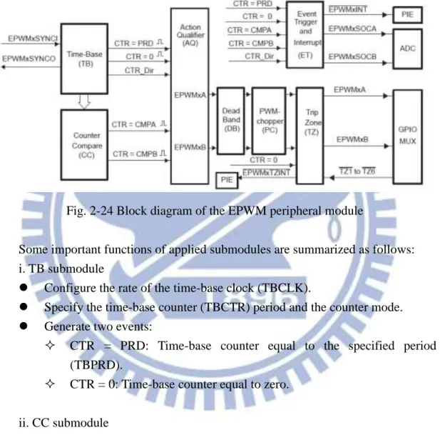
Fig. 2-24 Block diagram of the EPWM peripheral module ... 30

Fig. 2-25 Control signals for ideal switches ... 32

Fig. 2-26 Illustration of control signals of power switches ... 32

Fig. 2-27 Complete operation of the configured EPWM peripheral module ... 33

Fig. 2-28 Block diagram of the ADC peripheral module ... 34

Fig. 2-29 An example of the oversampling and the medium filter processing ... 35

Fig. 2-30 Input-output relationship of the system hardware ... 36

Fig. 2-31 Experimental reults of phase current signal recovery ... 36

Fig. 2-32 Block diagram of the EQEP peripheral module ... 37

Fig. 2-33 Output signals of an encoder with forward rotation ... 37

Fig. 2-35 Illustration of Capture unit operation ... 39

Fig. 3-1 Relationship between the estimated and actual d-q axis currents ... 42

Fig. 3-2 Control diagram of the rotor time constant identification process ... 43

Fig. 3-3 Responses with τˆ_r 0.08sandi_ds* i*_qs 0.4pu ... 44

Fig. 3-4 Experimental setup of rotor time constant identification without load ... 45

Fig. 3-5 Experimental results with different ˆ at no-load condition ... 46 _r Fig. 3-6 Experimental setup of rotor time constant identification performed directly on the vehicle ... 47

Fig. 3-7 Experimental results with different ˆ performed on the vehicle ... 47 _r Fig. 3-8 Speed response of practical driving ... 48

Fig. 3-9 Control diagram of obtaining the rotor flux linkage ... 51

Fig. 3-10 Experimental results of the d-axis current command 0.6 pu ... 52

Fig. 3-11 Experimental results of obtaining the rotor flux linkage ... 53

Fig. 3-12 Speed responses with the rated flux excitation ... 54

Fig. 3-13 Comparison of acceleration of the rated flux excitation and the equal d-q current command ... 54

Fig. 3-14 Setup of the standard experimental process ... 55

Fig. 3-15 Acceleration with different operated ids* ... 56

Fig. 3-16 Illustration of the input power of the inverter ... 57

Fig. 3-18 Speed response of the vehicle when ids* = 0.42 pu and 0.82 pu ... 59

Fig. 4-1 Relationship between the estimated and actual d-q axis currents ... 62

Fig. 4-2 Acceleration with different γ (ids* = 0.62 pu) ... 63

Fig. 4-3 Efficiency coefficient with different γ (ids* = 0.62 pu) ... 63

Fig. 4-4 Comparison of the speed response obtained bythe ids*-adjustment and the γ-adjustment ... 65

Fig. 4-5 Three stator current commands applied for the verification of torque ripples ... 66

Fig. 4-6 Comparison of the vehicular speed response operated at the maximum torque per amperage by the ids*-adjustment and the γ-adjustment ... 68

Fig. 4-7 Patterns of the testing switching process between the MTPA and the HE ... 69

Fig. 4-8 Results of the testing switching process obtained by the ids*-adjustment and the γ-adjustment ... 69

Fig. 4-9 Illustration of the designed switching strategy for γ ... 71

Fig. 4-10 Illustration of driving-condition checking of the switching strategy ... 71

Fig. 4-11 Classification of actions applied in operation 2 ... 73

Fig. 4-12 Flow chart of overall control program including the switching strategy ... 74

Fig. 4-13 Block diagram of overall control program implemented on the DSP controller ... 75

Fig. 4-14 Experimental results of operation with the MTPA, the HE, and the switching strategy ... 76

Fig. 4-16 Experimental results of control schemes with the switching strategy ... 80

Fig. 4-17 Speed responses obtained with different control strategies ... 81

Fig. 4-18 View of the inclined road for testing uphill climbing ability ... 82

List of Tables

Table 1-1 Performance comparison of different motors ... 1

Table 2-1 Datasheet of the lead-acid battery ... 23

Table 2-2 Datasheet of the power converter ... 23

Table 2-3 Nameplate of the induction machine ... 25

Table 2-4 Turn-off time of the power switches ... 33

Table 2-5 ADC channels in the control system board ... 34

Table 3-1 Experimental results of obtaining the rotor flux linkage ... 52

Table 3-2 Comparison of operations with ids* = 0.42 and 0.82 pu ... 58

Table 3-3 Comparison of the equal d-q current command and the rated flux excitation ... 60

Table 3-4 Comparison of the rated flux excitation and the highest efficiency operation ... 60

Table 4-1 Comparison of acceleration and efficiency ... 64

Table 4-2 Comparison of the ids*-adjustment and the γ-adjustment ... 65

Table 4-3 Definition of three operations in the switching strategy ... 71

Table 4-4 Comparison of with the MTPA, the HE, and the switching strategy ... 76

Chapter 1

Introduction

1.1 Motivation and Purposes

As the environmental quality is severely deteriorated by air pollution emitted from urban transportation as well as crude oil of the earth will be soon exhausted, electric vehicles have become major solutions for these crises and have been rapidly developed in recent years [1]-[2]. Among all components, the propulsion systems including electric machines and drives, are keys to electric vehicle design [3, 8].

It has been widely investigated in literatures [4]-[7] to indicate that the most commonly used types of machines are direct current motors (DCMs), permenant magnetic motors (PMs), and induction motors (IMs). Comparisons of their performance are listed in Table 1-1 [5]. Desite of fast response and control simplicity, DCMs have drawbacks such as low efficiency, low reliability, and frequent requests of maintenance due to the presence of machanical commutators and brushes, and thus their applications for electric vehicle are limited. Thanks to the recent development of electronics and control technologies, it is increasingly practical to introduce PMs and IMs to replace DCMs in traction applications. In fact, they are more attractive and desirable with high reliability and maintenance-free operations, which are prime considerations for electric propulsion sysytems.

Table 1-1 Performance comparison of different motors [5]

DCMs IMs PMs Power density ◎◎ ⊙ ⊕⊕ Efficiency ◎ ⊕ ⊕⊕ Costs ⊕ ⊕⊕ ◎ Reliability ◎ ⊕ ⊙ Technical maturity ⊕ ⊕ ⊙ ⊕⊕ ： Excellent ⊕ ： Good ⊙ ： Neutral ◎ ： Bad ◎◎ ： Unsatisfactory

The merits of the PMs are mainly in the inherent characteristics of high torque and power density. However, they are suffered from a limited speed operation range, lower overload capacity, and higher cost. Magnet corrosion and demagnetization are also potential problems for these motors. On the other hand, IMs are robust and capable of a wide speed range operation with reasonable cost in spite of comparatively low efficiency. As far as the current circumstances of electric machine selections for electric vehicles are concerned, PMs are chiefly preferred for their high torque and power density while IMs are mostly applied to high-power traction application as shown in Fig. 1-1 [22]-[23]. Yet, as the production of rare-earth metals uesd for manufacturing of permenant magnets becomes less in the future, the importance of IMs will increase in traction applications [24]-[25]. Therefore, a 0.75-kW IM is selected to propel an experimental electric vehicle in this Thesis, and the design of the traction control implemented on the DSP microcontroller to drive the electric machine and vehicle will be studied.

The field-oriented control or vector control scheme, which can obtain high dynamic performance servo control of IMs, has become an industrial standard for electric vehicle traction control [9]. It employs coordinate trasformation according to the position of the rotor flux linkage in order to realize independent dynamic control of the flux and torque of the machine. Based on the approach accessing the flux angle or the synchronous angle, vector control can be classified as the direct method and the indirect method [10]-[11]. In the former one, Hall sensors or flux sensing coils should be applied for the measurement. However, installing sensors around the air-gap is not preferred owing to the noise, armature reaction, space limitation, etc. A more reasonable way to identify the flux angle is via electical equations with voltage and current measurements. Nevertheless, it is still not reliable since the integration involved in the computation is difficult to implement with the fact that DC offsets are Fig. 1-1 Current circumstances of electric machine selections for electric vehicles [22]

DCMs IMs PMs Efficiency Power 1 kW 100 kW

inevitably present in voltage and current signals, especially at low rotational speed of the machine.

The indirect method, on the other hand, obtains the flux angle by exploiting the slip frequency calculated from the IM dynamic model and the motor shaft speed measured from encoders or resolvers. Such a method has become dominant in commercialized IM drive systems because performance of the instantaneous torque control is reliable from the start-up to the maximum speed of the machine. However, it is still challenging with pure indirect vector control to fulfill main requirements of traction performance such as large output torque and high operating efficiency for IM control [4, 15].

Hence, it is strongly motivated in this study to design and implement a DSP-based precise servo control of an IM which can maximize torque and efficiency and obtain smooth driving operation for an electric vehicle, as illustrated in Fig. 1-2. With such work, we expect that IMs become much more competitive in low-power traction applications.

Fig. 1-2 Illustration of research in this Thesis

Induction Motor Drive

Control strategy design:

(1) Maximum acceleration (2) Maximum efficiency (3) Driving smoothness Implementation DSP core: TMS320F28335

Induction Motor with 0.75kW Control Propulsion

1.2 Problem Statements

1. The key parameter of the IM involved in the implementation of servo control scheme is unknown

In order to obtain dynamic control of the flux and torque in the indirect vector control method, the rotor time constant is taken for the calculation of the slip frequency, on which the synchronous angle estimation is based. Thus, the decoupling of the stator current into flux and torque components is dependent on the rotor time constant [26]-[28]. Unfortunately, this parameter may not be accurately provided by the machine manufacturer. Without knowledge of the rotor time constant, the indirect vector control is unable to be implemented so that dynamic servo control of IM cannot be obtained.

2. Significant rolling resistance of the vehicle causes unsatisfactory acceleration

Total weight of the system that includes the driver and the vehicle is approximately 145 kg, and it leads to the 0.75-kW IM overloaded during the start-up period. If it is not properly operated, the generated torque will not be sufficient to provide satisfactory acceleration. Particularly, when the vehicle is driven on an inclined road, it may fail to complete uphill climbing and thus get trapped on the way or even slide backwards. To overcome this problem, the maximum torque per amperage (MTPA) control is to be introduced.

3. Operating efficiency and vehicle speed are limited with the MTPA operation

Although the torque can be maximally developed with the MTPA operation, it poses limitation on both operating efficiency and final speed of the vehicle due to strong excitation of the rotor flux linkage. When driven along a given route and distance, the vehicle with MTPA operation will consume more energy and take a longer time to complete the driving test.

4. Switching between operations results in uncomfortable driving experience

A control strategy by which operations can be adjusted according to driving requirements is encouraged to obtain both the MTPA and high efficiency operations. It can be achieved by altering operating flux of IM. However, it may cause unsteady driving operations with abrupt changes of the vehicle speed. Such phenomenon is undesirable for the real vehicle driving.

1.3 Proposed Approaches

1. An acceleration-based identification process directly performed on the vehicle is

developed to accurately obtain the rotor time constant

In general, the rotor time constant can be identified by a traditional identification approach including the no-load and locked-rotor tests [12]. However, extra instruments are required for power measurement and rotor locking in the process, and it is too difficult to realize them directly on the vehicle. On the other hand, we develop an alternative approach based on the acceleration information to obtain the rotor time constant in this study. The proposed identification process benefits from reasonable accuracy and simplicity of implementation on the vehicle.

2. Rated flux excitation is adopted for providing the MTPA operation

Basically, the MTPA operation indicates that the maximum torque can be produced at a given supplied stator phase current. It has been already recognized that by dividing the stator current equally into the flux-producing component and the torque-producing component, the MTPA operation can thus be obtained [13]. Yet, it is not suitable to the application in this study since severe flux saturation occurs and the desirable MTPA operation is lost. Another common suggestion is that the rotor flux linkage is excited at its rated level [10, 14]. The determination of the operating flux current corresponding to the rated rotor flux linkage is first derived based on the IM dynamic model. Then, a standard experimental process used for testing vehicle acceleration is established for the verification. Results show that the MTPA operation can be obtained by the rated flux excitation.

3. The standard experimental process testing efficiency is employed to find the highest efficieny (HE) operation

By regulating the rotor flux linkage at an appropriate level, the highest operating efficiency of the IM can be obtained [16]-[17]. We utilize the developed experimental process to test efficiency with different settings of the flux current. It is verified from the experimental results that the HE operation can be obtained by operating the IM at a smaller flux level.

4. A smooth switching strategy based on the proposed slip factor adjustment

(γ-adjustment) is designed to achieve both the MTPA and the HE operation As previously described, both operating efficiency and final speed of the

vehicle is limited with MTPA operation. Apparently, it is unfavorable to always be regulated at this operation for traction applications of IM. Firstly, we propose a novel control method by adjusting the defined slip factor γ, and both the MTPA as well as the HE operation can thus be obtained. Then, a switching strategy with which the MTPA operation is applied at a low speed for the maximum acceleration while the HE operation is applied to the high speed for improved operating efficiency and vehicle speed is designed based on the γ-adjustment. It has also been proved that the designed strategy can obtain smooth driving operations, and thus it is more suitable to traction control of electric vehicles.

1.4 Organization of the Thesis

The thesis is arranged as follows. Chapter 1 describes main purposes and goals of the research as well as general review of technical development. Research problems and their corresponding solutions are stated in this chapter as well; Chapter 2 examines relevant technical background, including modeling, analysis, and dynamic control of an induction machine. Then, the experimental system applied in the research is introduced; Chapter 3 presents the servo control of the induction machine used for the traction application. Rotor time constant identification, maximum torque per amperage control, and operating efficiency are involved in the investigation; Chapter 4 demonstrates an automatic switching strategy fulfilling both requirements of the maximum acceleration and the highest operating efficiency. Novel γ-adjustment control method developed for smooth driving performance is also described and verified in this chapter. Finally, achievements and contributions of the thesis are summarized in Chapter 5.

Chapter 2

Technical Background and System

Structure

Although operating principles of an induction machine are similar to those of a transformer, its analysis and modeling become more complicated due to rotation of the secondary winding, i.e. the rotor of the machine. This is primarily because the inductances vary at different rotor position, and the electrical differential equations are time-varying as long as the rotor rotates. Theory of the reference frame transformation has been developed to transform the time-varing equations into the time-invariant ones to simplify the mathematical analysis of an induction motor. Then, high performance vector control was formulated for servo control of an induction motor based on its dynamic model. In this chapter, technical background with respect to modeling, analysis, and dynamic control of an induction machine will be introduced, followed by the system layout of the experimental electric vehicle driven with a single induction motor.

2.1 Transformation of Reference Frame

The illustration of a three-phase a-b-c axis, a stationary refernce frame d-q axis (superscripted as s), and a rotating reference frame d-q axis (superscripted as ω) with arbitraty speed, ω, is shown in Fig. 2-1.

Fig. 2-1 Relationship between reference frames

a (Realaxis) s d 

q



 b c axis) (Imaginary s q 

d

abc f

An arbitrary space vector in the three-phase system can be defined as ) ( 3 2 2/3 j2/3 cs j bs as abc f f e f e f     (2-1)

Refered to the stationary reference frame, it can expressed as

abc s qs s ds s dq f jf f f     (2-2) Thus, the transformation matrix converting a variable in the three-phase axis into the stationary frame can be derived as

                               2 3 2 3 0 2 1 2 1 1 3 2 3 2 sin ) 3 2 sin( 0 3 2 cos ) 3 2 cos( 1 3 2     C (2-3) such that                    cs bs as s qs s ds f f f f f C (2-4)

Since the instantaneous angle between the d axis of the rotating reference frame and the stationary real axis is θ as illustrated in Fig. 2-1, the variable in the equation (2-1) can be further referred to the rotating reference frame as

    s j dq qs ds dq f jf f e f      (2-5) Then, the relationship of its components expressed in these two reference frames are given by                      qs ds qs ds f f f f P (2-6)

where P is the transformation matrix, which can be represented as

            cos sin sin cos P (2-7)

2.2 Dynamic Charactersitics of an Induction Machine

Three-phase axis of the stator (as-bs-cs) and rotor (ar-br-cr) of an induction motor is shown in Fig. 2-2. The ar-br-cr axis rotates with electrical speed, ωr, as

the machine is P, the relationship between the mechanical speed and the electrical speed is given by m r P_  2  (2-8) as derived from m r P_  2  (2-9)

Therefore, the stator and rotor electical equations can be written in vector form as

abcs abcs s abcs R I pλ V   (2-10) abcr abcr r abcr RI pλ V   (2-11)

where p stands for a differential operator, Rs is the stator winding resistance, Rr is the

rotor winding resistance referred to the stator side, and each vector term is given by





T cs bs as abcs  V V V V (2-12)





T cs bs as abcs  i i i I (2-13)





T cs bs as abcs    λ (2-14)





T cr br ar abcr  V V V V (2-15)





T cr br ar abcr  i i i I (2-16)





T cr br ar abcr     λ (2-17) Fig. 2-2 Three-phase axis of the stator and rotor

as bs cs ar br cr r



r



The flux linkages for the stator and rotor can be expressed as                    abcr abcs r T sr sr s abcr abcs I I L L L L λ λ (2-18) where                           ms ls ms ms ms ms ls ms ms ms ms ls s L L L L L L L L L L L L 2 1 2 1 2 1 2 1 2 1 2 1 L (2-19)                           mr lr mr mr mr mr lr mr mr mr mr lr r L L L L L L L L L L L L 2 1 2 1 2 1 2 1 2 1 2 1 L (2-20)                        r r r r r r r r r sr sr L                cos ) 3 2 cos( ) 3 2 cos( ) 3 2 cos( cos ) 3 2 cos( ) 3 2 cos( ) 3 2 cos( cos L (2-21)

In the equation (2-19) ~ (2-21), Lls is the leakage inductance of the stator

winding, Llr stands for the leakage inductance of the rotor winding, and Lms and Lmr is

the mutual inductance of the stator and the rotor, respectively. Lsr means the mutual

inductance between the a-phase stator winding and the a-phase rotor winding when θr

is zero. As seen from (2-10) ~ (2-21), the equations describing the dynamic characteritics of the induction motor are time-varying. Obviously, it is considerably difficult to solve such sophisticated differential equations analytically. However, if the coordinate transformation by which the three-phase variables are transformed into d-q variables as described in Section 2.1, electrical equations with time-invariant form can be obtained, and thus the induction machine becomes simple to analyze. The deduction from time-varying equations to time-invariant ones in detail is described in [10].

The d-q stator and rotor voltage equations at reference frame with arbitrary rotational speed can be expressed as

    _{ } qs ds ds s ds R i p V    (2-22)

    _{ } ds qs qs s qs R i p V    (2-23)     _{   } qr r dr dr r dr R i p V   (  ) (2-24)     _{   } dr r qr qr r qr R i p V   (  ) (2-25) where the electrical speed of the rotor’s rotation is ωr. Particularly, the rotor voltage is

zero in the case of squirrel-cage induction motor, i.e. singly-fed induction motor, since the rotor is short-circuited by the end ring. As a consequence, (2-24) and (2-25) become    _{   } qr r dr dr ri p R ( ) 0    (2-26)    _{   } dr r qr qr ri p R ( ) 0    (2-27) The flux linkage of the stator and rotor can also be represented in terms of d-q variables as    _ds L_si_ds L_mi_dr (2-28)    _qs L_si_qs L_mi_qr (2-29)    _dr L_mi_dsL_ri_dr (2-30)    _qr L_mi_qsL_ri_qr (2-31) where L_m  L_ms,L_s L_m L_ls,L_r L_m L_lr 2 3

. Finally, the electromagnetic torque can be represented as ) ( 2 2 3 _{   } ds qr qs dr r m e i i L L P T   (2-32)

Based on the equation (2-22)-(2-31), the equivalent circuit of the squirrel-cage induction machine at an arbitrary speed rotating d-q reference frame can be depicted as Fig. 2-3. (a) d-axis  ds V   s R L_ls m L lr L  ds i r R  ds     r) dr (   dr i 0   dr V     ds _dr          

2.3 Indirect Vector Control

2.3.1 Principles of indirect vector control

The electrical equations at the synchronously rotating d-q reference frame can be derived by subsituting ω = ωe in (2-22), (2-23), (2-26), and (2-27), and all the

superscipts, ω, in the equations are omitted for expression at the synchronous reference frame. Then, the dynamic charateristics at the synchronous reference frame can be expressed as qs e ds ds s ds Ri p V      (2-33) ds e qs qs s qs Ri p V      (2-34) qr r e dr dr ri p R  (  ) 0    (2-35) dr r e qr qr ri p R  (  ) 0    (2-36)

where the flux linkage terms are given by

dr m ds s ds L i L i  (2-37) qr m qs s qs L i L i  (2-38) dr r ds m dr L i Li  (2-39) qr r qs m qr L i L i  (2-40) Indirect vector control is performed based on the assumption that the rotor flux linkage only exists on the d axis. In other words,

e qr e qr p  0 (2-41) (b) q-axis

Fig. 2-3 Equivalent circuit of the squirrel-cage induction motor

 qs V   s R L_ls m L lr L  qs i r R  ds  _{  } qr r) (   qr i 0   qr V     qs _qr          

By substituting (2-41) into (2-35), (2-36), and (2-40), we can obtain the following equations respectively. r dr dr R p i   (2-42) dr qr r r e slip i R        (2-43) qs r m qr i L L i  (2-44) The rotor flux linkage in s-domain can be derived by substituting (2-42) into (2-39) with Laplace transform as

s i L r ds m dr _    1 (2-45) where_r L /_r R_rdenotes the rotor time constant. Then, we subsitute (2-44) and (2-45) into (2-43), the slip angular frequency can be expressed in terms of the d-axis current and the q-axis current as

ds qs r r slip i i s    1 (2-46) Finally, the electromagnetic torque can be simplified with the absent q-axis rotor flux linkage as qs dr r m e i L L P T  2 2 3  (2-47) Hence, the torque is directly proportional to the q-axis current under the condition that the rotor flux linkage is constant. Furthermore, the rotor flux linkage is excited solely by the d-axis current as seen from (2-45). Therefore, the d-axis current is also named as the flux-producing current and the q-axis current is called the torque-producing current. Obviously, the behavior of the indiect vector-controlled induction motor is quite similar to that of a separately excited DC machine, and thus the dynamic response of the induction machine can be controlled.

2.3.2 Implementation of indirect vector control

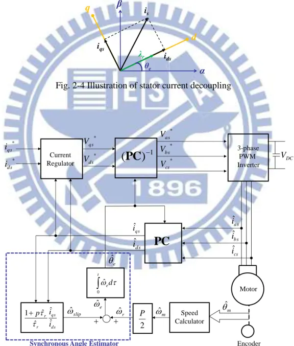
In order to implement the described control process, the knowledge of angular position of the rotor flux linkage is essential since the d axis is supposed to be aligned with it so that the stator phase current can be divided into the flux-producing and torque-producing components as illustrated in Fig. 2-4. The angular position of the rotor flux, i.e. the synchronous angle, can be estimated indirectly by integrating the

calculated electrical angular frequency as





   t _e t _{r slip} e d d 0 0 ) ˆ ˆ ( ˆ ˆ _{    }  (2-48)

Obviously, the slip frequency is involved and summed with the angular rotor shaft speed in electrical angle, ˆ . Thus, the rotor time constant of the machine must be _r known, and the performance is highly dependent on this parameter. The control block diagram of indirect vector control of an induction motor is shown in Fig. 2-5.

Fig. 2-4 Illustration of stator current decoupling

α β i_s i_ds i_qs λ_r d q θ_e

Fig. 2-5 Block diagram of indirect vector control

* ds i * qs i 3-phase PWM Inverter Motor Encoder Speed Calculator m ˆ * as V * bs V * cs V 1

)

(

PC

 VDC as iˆ bs iˆ cs iˆ

PC

ds qs r r i i p ˆ ˆ ˆ ˆ 1     d t e



0 ˆ m ˆ slip ˆ ˆe e ˆ   ds iˆ qs iˆ Current Regulator * qs V * ds V

Synchronous Angle Estimator 2

P r ˆ

As seen from Fig. 2-5, a current-regulated pulse width modulation (PWM) inverter is applied to control the d-q components current of the motor. In particular, the block with the notation PC is the coordinate transformation from the three-phase system to the synchronous reference frame, employing the transformation matrix which is the multiplication of P and C as presented in (2-3) and (2-7). On the other

hand, the block with the notation (PC)-1 indicates the inverse coordinate

transformation transforming the variables in the synchronous reference frame back to those in the three-phase coordinate. Finally, the synchronous angle estimator, which is composed of the slip frequency estimation and the integration of the synchronously rotating speed, is responsible for providing the synchronous angle for the coordinate transformation.

2.3.3 Dynamic model of an indirect vector-controlled induction motor

The d-q stator voltage can be expressed in terms of the stator current and rotor flux linkage based on the rotor flux linkage orientation of the vector control as

qs s e dr r m ds s ds s ds L i dt d L L dt di L i R V      (2-49) ds s e dr e r m qs s qs s qs Li L L dt di L i R V       (2-50) where r s m L L L2 1 

 stands for the total leakage factor. In (2-50), the terms

) ( _{dr s ds} r m e ds s e dr e r m i L L L i L L L           (2-51) ) ( m dr s dr r m e L L L L       (2-52) dr m s e L L   ( )  dr m s slip m L L P_{  } ) )( 2 (   dr m s slip dr m s m L L L L P_{   } ) ( ) ( 2   (2-53)

If the variation of the flux linkage is sufficiently slow compared with the rotor time constant, it can be obtained by substituting p=0 in (2-45) as

ds m dr L i

 (2-54) for deriving (2-52) from (2-51). Similarly, the slip frequency can be written as

ds qs r slip i i    1 (2-55) Therefore, the equation (2-56) can be derived by substituting (2-55) into (2-53) as

qs r r s dr m m s ds s e dr e r m i R L L L L P i L L L        2 (2-56)

Substitute (2-56) into (2-50) and take the Laplace transform on the both side of the equal sign, and we can derive

) ( 1 _{e dr e s ds} r m qs s s qs Li L L V R s L i         ) 2 ( 1 _{r qs} r s dr m m s qs s s i R L L L L P V R s L        ) 2 ( ) ( 1 _{m dr} m s qs r r s s s L L P V R L L R s L        (2-57)

where the term _{m dr}

m s

L L P _{ }

2 indicates the back electromagnetic force (back-emf), Vb.

In general, the machanical dynamics of an induction motor can be expressed as

m m L e B dt d J T T      (2-58)

where TL is the applied mechanical load, J stands for the inertia, and B indicates the

viscous friction coefficient. Thus, based on (2-47), (2-57), and (2-58) the dynamic model of the indirect vector-controlled induction motor can be depicted as Fig. 2-6.

The torque and back-emf constant of the induction motor can be defined as Kt

and Ke, respectively, such that dr r m t qs t e L L P K i K T  4 3 ,   (2-59) dr m s e m e b L L P K K V   2 ,   (2-60) Fig. 2-6 Dynamic model of the indirect vector-controlled induction motor

) ( 1 r r s s s R L L R s L    qs V e T B Js 1 m L T  dr r m L L P _ 4 3 qs i dr m s L L P _ 2

Consequently, performance of the induction machine is determined by the condition of the rotor flux linkage. It is also the major concern of this study and it will be discussed and verified in detail in next chapter.

2.4 Operation Region of an Induction Machine

2.4.1 Voltage and current constraints on induction machine control

Due to components and input voltage of the power inverter, the electric power delivering to the machine is limited by the voltage and current ratings. Even though the inverter has sufficiently large ratings, the machine itself has constraints owing to insulation and thermal limit. In control of the induction machine, both the voltage and current constraints must be considered.

The maximum phase voltage of the motor, Vsmax, is determined by the DC-bus

voltage of the inverter while the maximum current flowing into the machine, Ismax, is

limited by the thermal rating of the inverter or the machine itself. Thus, the following two constraints must be hold:

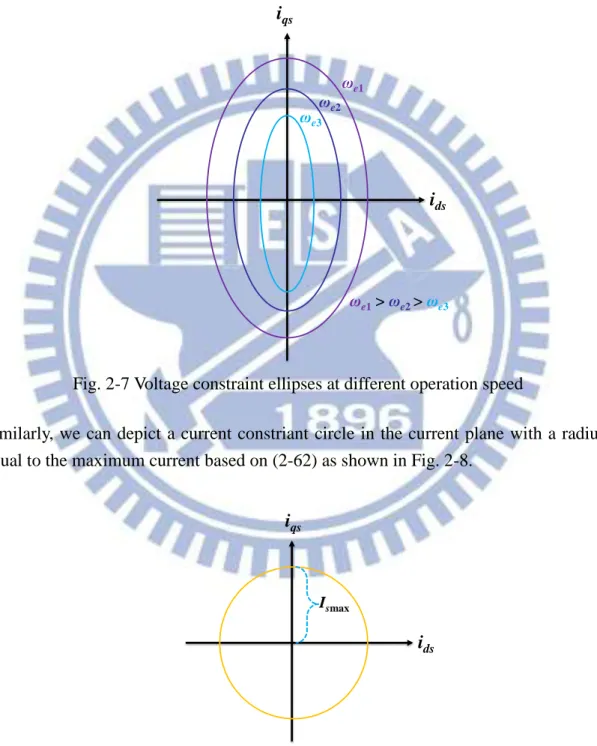
max 2 2 2 s s qs ds V V V V    (2-61) max 2 2 2 s s qs ds i i I i    (2-62) The equations (2-49) and (2-50) can be simplified as (2-61) and (2-62) under the steady-state operation. qs s e ds s ds Ri Li V    (2-63) ds s e qs s qs Ri Li V   (2-64) A further simplification can be obtained by neglecting the voltage drop over the stator resistance as qs s e ds L i V  (2-65) ds s e qs L i V  (2-66) By substituting (2-63) and (2-64) into the voltage constraint shown in (2-61), an ineqality representing an ellipse in the synchronous reference current plane can be obtained as follows.

1 ) ( ) ( max 2 2 2 max 2   s e s qs s e s ds L V i L V i    (2-67)

Since σ is typically equal to 0.1, the major axis lies on the iqs-axis while the minor

axis lies on the ids-axis. Fig. 2-7 illustrates ellipses of the voltage constraint at

different operation speed.

Similarly, we can depict a current constriant circle in the current plane with a radius equal to the maximum current based on (2-62) as shown in Fig. 2-8.

Fig. 2-7 Voltage constraint ellipses at different operation speed

i_ds i_qs ω_e1 ω_e2 ω_e3 ω_e1>ω_e2 >ω_e3

Fig. 2-8 Circle of current constraint

i_ds i_qs

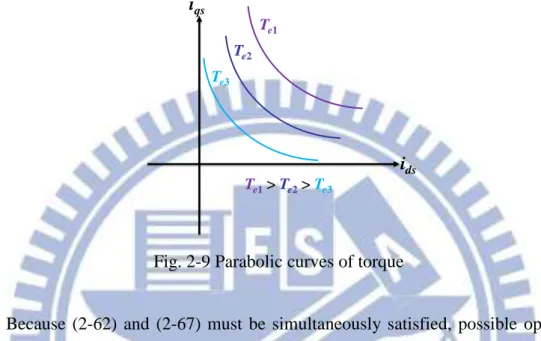
The torque shown in (2-47) can be derived as qs ds r m e i i L L P T 2 2 2 3  (2-68) Hence, the developed torque of the induction machine can also be plotted in the current plane and it appears as a parabolic curve. The illustration is shown in Fig. 2-9.

Because (2-62) and (2-67) must be simultaneously satisfied, possible operating point lies in the cross secrion of the voltage constraint ellipse and the current constraint circle, as the shaded area shown in Fig. 2-10. The torque at a specific operation point is determined by the product of the d-axis and q-axis components current.

Fig. 2-9 Parabolic curves of torque

i_ds i_qs T_e1 T_e2 T_e3 Te1>Te2>Te3

Fig. 2-10 Possible operation points considering both voltage and current constraint

ids i_qs qs ds r m e i i L L P T 2 2 2 3 

2.4.2 Capability curve of an induction machine

The operation region of an induction machine can be basically categorized into three regions. The first region, indicating the frequency from zero to the base frequency, is called the constant torque region. In this region, the maximum torque is limited by the maximum stator current, which is determined by Ismax. At the base

frequency, the terminal voltage of the motor reaches the voltage limit.

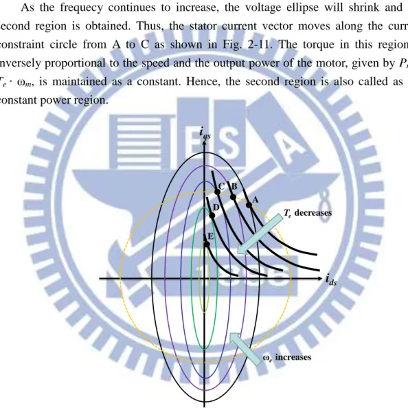
As the frequecy continues to increase, the voltage ellipse will shrink and the second region is obtained. Thus, the stator current vector moves along the current constraint circle from A to C as shown in Fig. 2-11. The torque in this region is

inversely proportional to the speed and the output power of the motor, given by Pm =

Te ∙ ωm, is maintained as a constant. Hence, the second region is also called as the

constant power region.

If the operating frequency further increases above point C, the volatge ellipse will shrink inside the current limit circle to enter the third region, and there is no crossing point between the ellipse and the circle as E and F shown in Fig. 2-11. In this case, the operation is completely limited by the voltage constriant. Since the current

Fig. 2-11 Locus of voltage ellipse, current circle, and torque in different operation regions

i_ds i_qs A B C D E ω_e increases Te decreases

also decreases as the frequency increases, the torque decreases inversely proportional to the square of ωe. This region is called as the characteritic region of the induction

motor.

The torque, stator volatge, and stator current can be plotted versus the electrical frequency to specify these three operation region as shown in Fig. 2-12. The curve is also known as the capability curve or the characteristic curve of the induction machine.

2.5 System Structure

2.5.1 Mechanical layout of the electric vehicle

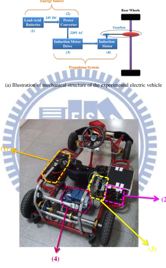
The overall mechanical scheme of the electric vehicle adopted in this study is shown in Fig. 2-13. The components corresponding to the number marked in Fig. 2-13 are described as below.

Fig. 2-12 Capability Curve of an induction motor

Constant torque region Constant power region T_e Vs ω_e ω_b Characteristic region I_s e e T  1  2 1 e e T   Ismax V_smax

(b) The experimental electric vehicle

Fig. 2-13 Overall structure of the experimental electric vehicle

(1)

(2)

(3)

(4)

(a) Illustration of mechanical structure of the experimental electric vehicle

Lead-Acid Batteries 24V DC Power Converter Induction Motor Drive 220V AC Induction Motor Gearbox (1) (2) (3) (4) Rear Wheels Energy Source Propulsion System

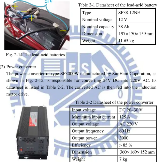
(1) Lead-acid batteries

Energy source is provided by two lead-acid batteries in series connection manufactured by Tinshfom Coporation. The voltage is 24V in total as shown in Fig. 2-14. The datasheet of the battery is listed in Table 2-1.

(2) Power converter

The power converter of type SP3000W manufactured by SunHam Coporation, as shown in Fig. 2-15, is responsible for converting 24V DC into 220V AC. Its datasheet is listed in Table 2-2. The converted AC is then fed into the induction motor drive.

(3) Induction motor drive

The induction motor drive is composed of a power stage module and a control system module, as shown in Fig. 2-16. Basically, the power stage module can be divided into two parts: a three-phase bridge rectifier and a three-phase inverter. The former one rectifies AC input to a DC, providing electromotive force for the DC-bus. Then, three legs of IGBTs (Insulated Gate Bipolar Transistor) are Fig. 2-15 The power converter

Fig. 2-14 The lead-acid batteries

＋

－

＋

－

24 V

Table 2-2 Datasheet of the power converter

Input voltage DC 20~30 V

Maximum input current 125 A

Output voltage AC 220 V Output frequency 60 Hz Output power 3000 Efficiency > 85 % Dimension 360169152mm Weight 7 kg

Table 2-1 Datasheet of the lead-acid battery

Type SP38-12NE

Nominal voltage 12 V

Nominal capacity 38 Ah

Dimension 197130159mm

controlled by the control system module to generate proper AC for the motor. The illustration of the induction motor drive is shown in Fig. 2-17.

Fig. 2-17 Illustration of the induction motor drive

AC power source

AC-to-DC DC-to-AC

Power stage module

Control system module

I/O signals

Encoder signals

Induction Motor Drive

Motor dc V 1 Q 2 Q 3 Q 4 Q 5 Q 6 Q U V W

Fig. 2-16 The induction motor drive

Induction Motor Drive

Control System Module

The power stage module is manufactured by Long-Shenq Electronic Corporation, whose product type is LS800-22K2-TD, while the control system module is developed by Syntec Incorporation. The DSP controller of type TMS320F28335 manufactured by the Texas Instruments is the processing core. Its detailed features and functions can be found in [18].

(4) Induction machine

A three-phase squirrel-cage induction motor with 0.75 kW as shown in Fig. 2-18 is applied to the propulsion of the vehicle. Its nameplate is shown in Table 2-3.

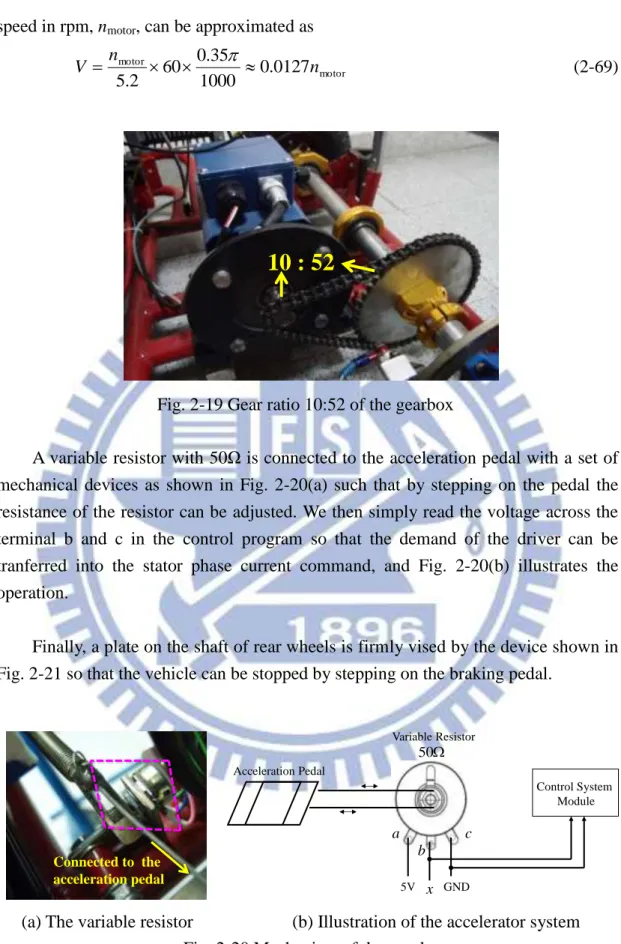
The mechanical power is transmitted from the induction motor to the rear wheels with a gear ratio at 10:52, as shown in Fig. 2-19. Because the diameter of the rear wheel is around 35 cm, the speed of the vehicle in km/hr, V, at given motor rotational

Table 2-3 Nameplate of the induction machine

Manufacturer Cheng-Chang Machine Eletronic Corporation

Type SVM-80SS Rated power 0.75 kW Rated frequency 51.5 Hz Rated slip 45 rpm Rated speed 1500 rpm Rated torque 4.7 N-m

Rated line Voltage Y connection 380 V

Δ connection 220 V

Rated line Current Y connection 1.9 A

Δ connection 3.3 A

Weight 13.56 kg

Encoder resolution 1024 pulses per revolution (ppr)

speed in rpm, nmotor, can be approximated as motor motor 0127 . 0 1000 35 . 0 60 2 . 5 n n V      (2-69)

A variable resistor with 50Ω is connected to the acceleration pedal with a set of mechanical devices as shown in Fig. 2-20(a) such that by stepping on the pedal the resistance of the resistor can be adjusted. We then simply read the voltage across the terminal b and c in the control program so that the demand of the driver can be tranferred into the stator phase current command, and Fig. 2-20(b) illustrates the operation.

Finally, a plate on the shaft of rear wheels is firmly vised by the device shown in Fig. 2-21 so that the vehicle can be stopped by stepping on the braking pedal.

Fig. 2-19 Gear ratio 10:52 of the gearbox

10 : 52

(a) The variable resistor (b) Illustration of the accelerator system Fig. 2-20 Mechanism of the accelerator

Connected to the acceleration pedal Variable Resistor Acceleration Pedal  50 5V _x GND Control System Module a b c

2.5.2 Control program of the system

The indirect vector control is exploited as the traction control of the electric vehicle in this study, which is fully digitized and implemented on the DSP controller. The block diagram of the control scheme is shown in Fig. 2-22.

Fig. 2-21 The braking mechanism

Connected to the braking pedal Vising for brake

Fig. 2-22 Control scheme implemented on the DSP controller

PI * ds i PI * qs i Inverse Coordinate Transformation Synchronous Angle Estimator Coordinate Transformation ADC Peripheral EQEP Peripheral SVPWM EPWM Peripheral 3-phase Inverter Motor Encoder Control signals Speed Calculator e ˆ qs iˆ ds iˆ m ˆ ph s iˆ_3 3 1~ S S m ˆ Accelerator Signal Driver’s Demand * ds V * qs V * 3 ph s V  lim  s i Component Assignment * s i Sampling frequency：15 kHz

As illustrated in Fig. 2-22, the driver’s demand is transferred into the stator current command followed by the component assignment, which is functional as dividing the given stator current command into d-q current commands. The d-axis current command is normally selected as a constant value. Then, the q-axis current command is determined by 2 * 2 * * ds s qs i i i   (2-70) Particularly, a switch connected to 5V-source is used for specifying forward or backward driving. The vehicle is operated at forward driving mode when the switch is off, and the q-axis current command is set as (2-70). When the switch is on, the q-axis current command is set as negative for reverse rotation of the machine. Since the maximum stator current is determined by the thermal rating of the motor and the inverter as discussed in Section 2.4.1, the stator current command is limited by is-lim,

2.576 pu (1 pu stands for 3.3 A in the system).

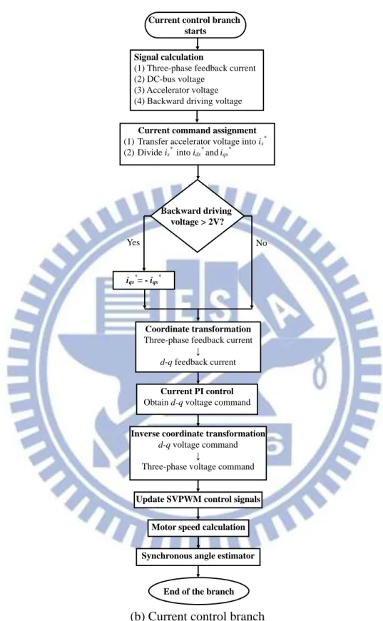
Two PI controllers are presented for current regulation, generating d-q voltage commands. Then, transformation between the three-phase system and the synchronous reference frame is managed by the blocks of coordinate transformation and inverse coordinate transformation, which is based on the estimated synchronous angle provided by the synchronous angle estimator, as discussed in Section 2.3.2. Finally, to generate appropriate control signals according to the three-phase voltage commands for the inverter, the space vector pulse width modulation (SVPWM) approach is applied. The flow chart of the control program is illustrated in Fig. 2-23, and the sampling frequency of the system is 15 kHz.

(a) Main program

Program starts

System initialization

(1) Variable declaration

(2) Configure and enable peripheral module

Interrupt request received?

Current control branch

No

Fig. 2-23 Flow chart of the control program

There are three processing modules, i.e. EPWM, ADC, and EQEP peripherals, of the DSP controller that play an important role in the control scheme. Their functions and relevant configurations are briefly described as below.

(b) Current control branch

Current control branch starts

Signal calculation

(1) Three-phase feedback current (2) DC-bus voltage

(3) Accelerator voltage (4) Backward driving voltage

Current command assignment

(1) Transfer accelerator voltage into is* (2) Divide is* into ids* and iqs*

Backward driving voltage > 2V?

iqs*= - iqs*

Yes No

Coordinate transformation

Three-phase feedback current ↓

d-q feedback current

Current PI control

Obtain d-q voltage command

Inverse coordinate transformation

d-q voltage command ↓

Three-phase voltage command

Update SVPWM control signals Motor speed calculation

Synchronous angle estimator