具關連性多輸入多輸出系統之位元分配與傳送器設計

國

立

交

通

大

學

電控工程研究所

碩

士

論

文

具關連性多輸入多輸出系統之位元分配與傳送器設計

Joint Design of Statistical Precoder and Statistical Bit Allocation for Correlated MIMO Channels

研 究 生：蕭君維

指導教授：林源倍 博士

具關連性多輸入多輸出系統之位元分配與傳送器設計

Joint Design of Statistical Precoder and Statistical Bit Allocation for Correlated MIMO Channels

研 究 生：蕭君維 Student：Chun-Wei Hsiao

指導教授：林源倍 Advisor：Yuan-Pei Lin

國 立 交 通 大 學

電控工程研究所

碩 士 論 文

Submitted to Department of Control Engineering College of Electrical Engineering

National Chiao Tung University in partial Fulfillment of the Requirements

for the Degree of Master

in

Department of Electrical Engineering

November 2011

具關連性多輸入多輸出系統之位元分配與傳送器設計

研究生：蕭君維

指導教授：林源倍 博士

國立交通大學電控工程研究所碩士班

摘要

在本篇論文中，我們提出對於輸入端具關連性多輸入多輸出系統，其

位元配置與傳送器的設計方法。首先我們根據具關連性通道之錯誤變

異係數的統計特性推導出最佳位元配置與平均錯誤率下限，接著我們

設計出能最小化平均錯誤率下限之傳送器與最適合的通道數目。模擬

結果顯示我們所提出的方法可以有效降低具關連性多輸入多輸出系

統之錯誤率。

致謝

碩班這兩年多來，在研究與做事態度上很感謝林源倍教授的指導，

這學習過程對我來講是份特別的經歷。感謝陳伯寧教授、吳卓諭教授

以及蔡尚澕教授，撥冗參加我的畢業口試並提供很不錯的建議讓我的

論文更加完善，更要謝謝你們的鼓勵。感謝實驗室建璋大學長、虹君、

人予、士傑、超任、子軒、奇璋，大家對於實驗室氣氛不遺餘力的經

營，有你們在實驗室生活變得多彩而有意義。

特別感謝大學同學小蔡長期提供舒適的窩，讓我在最後階段無後顧

之憂完成碩士論文。當然也要謝謝這些日子來，與我一起消遣遊樂的

好同學好朋友們。最後的最後謝謝爸爸媽媽一路來給我最安穩的避風

港。

Joint Design of Statistical Precoder and

Statistical Bit Allocation for Correlated

MIMO Channels

Chunwei Hsiao

Advisor: Dr. Yuan-Pei Lin

Department of Electrical Engineering

National Chiao Tung University

Abstract

In this thesis we consider the design of statistical precoder and sta-tistical bit allocation for multi-input multi-output (MIMO) systems over correlated channels. We assume the correlated channel is slow fading and full channel state information is available at the receiver, while only the statistics of the correlated channels is assumed to be known at transmitter. We will first derive the statistical bound of bit error rate (BER) and the corresponding optimal real bit allocation. Based on this statistical BER bound, the optimal unitary statisti-cal precoder is derived both for linear and decision feedback receiver. Second, the statistical integer bit allocation is designed the greedy al-gorithm. Finally, different number of substreams will be considered

and selected by statistical BER bound. Simulations show lower BER can be achieved when optimal number of substreams is selected for correlated channels.

Contents

1 Introductions 1

1.1 Outline . . . 3

1.2 Notations . . . 3

2 General System Model 4 2.1 Statistical Bit Allocation System Model . . . 4

2.2 Receiver Design . . . 5

2.2.1 Linear receiver . . . 5

2.2.2 Decision feedback receiver . . . 6

3 Previous Works of Statistical Designs 10 3.1 Statistical Precoders for Linear Receivers . . . 10

3.2 Statistical Precoders for Decision Feedback Receivers . . . 11

3.3 Statistical Bit Allocation with Decision Feedback Receiver . . 13

3.3.1 Statistical bit allocation for i.i.d. channel . . . 13

3.3.2 Statistical bit allocation for correlated channel . . . 14

4 Statistical Precoder Design 15 4.1 Derivation of Statistical BER Bound and Optimal Real Bit Allocation . . . 15

4.2 Precoder Design . . . 17

4.3 Design of Integer Bit Allocation . . . 20

4.3.1 Minimum BER bit allocation (bmber) . . . 20

4.3.2 Most probable bit allocation (bprob) . . . 20

4.3.3 Bit allocation using greedy algorithm (bgr,M) . . . 21

4.3.4 Bit allocation for minimizing statistical bound (bd,M) . 22 4.3.5 Optimal number of substream Mopt . . . 22

5 Simulation Result 24

List of Figures

2.1 The system model of MIMO transmission system. . . 5 2.2 Block diagram of the decision feedback receiver based on QR

decomposition. . . 6 5.1 Example 1.A. Different Integer Bit Allocation schemes (Mr =

4, Mt= 3, M = 3, Rb = 12) for (a) ρ =0, (b) ρ =0.5, and (c)

ρ =0.9. . . . 26 5.2 Example 1.B. Different Integer Bit Allocation schemes (Mr =

6, Mt= 4, M = 4, Rb = 8) for (a) ρ =0, (b) ρ =0.3, and (c)

ρ =0.7. . . . 28 5.3 Example 2.A. Performance for different Vf (Mr = 6, Mt =

4, M = 4, Rb = 18) for (a) bgr,4, (b) breal,4 and (c) breal,4

with high bit rate assumption. . . 31 5.4 Example 3.A. Performance for different M0 (Mr = 4, Mt =

3, M = 3, Rb = 12) for (a) ρ = 0, Mopt = 3, (b) ρ =

0.5, Mopt = 3 and (c) ρ = 0.9, Mopt= 2. . . . 33

5.5 Example 3.B. Performance for different M0 (Mr = 6, Mt =

4, M = 4, Rb = 8) for (a) ρ = 0, Mopt = 3, (b) ρ =

0.3, Mopt = 3 and (c) ρ = 0.7, Mopt= 2. . . 35

5.6 Example 4.A. Performance of different precoders for uniform bit allocation. (a) ρ =0.5; (b) ρ =0.9. . . . 37 5.7 Example 4.B. Performance of different precoders when the bit

allocation is bgr,M. (a) ρ =0.5, bgr,M = [8 6 4]; (b) ρ =0.9,

bgr,M = [10 5 3]. . . 39

5.8 Example 5.A. Performance for different ρ (Mr = 6, Mt =

4, M = 4) for (a) Rb = 8, and (b) Rb = 12. . . 40

5.9 Example 5.B. Comparison of improvement gain (Mr = 6, Mt=

5.10 Example 6.A. Comparison of different detection orderings for (Mr = 4, Mt = 3, M = 3, Rb = 18, ρ = 0.5) (a) uniform bit

allocation, and (b) bgr,Mopt = [8 6 4]. . . 43

5.11 Example 6.B. Comparison of different detection ordering (Mr =

6, Mt= 4, M = 4, Rb = 8, ρ = 0) for (a) uniform bit

alloca-tion, and (b) bgr,Mopt = [3 3 2]. . . 45

5.12 Example 7.A. Comparison with other related works (Mr =

4, Mt = 3, M = 3, Rb = 12) for (a) ρ =0, bgr,Mopt=(5 4 3)

(b) ρ =0.5, bgr,Mopt=(6 4 2) and (c) ρ =0.9, bgr,Mopt=(8 4). . . 48

5.13 Example 7.B. Comparison with other related works (Mr =

4, Mt = 3, M = 3, Rb = 18) for (a) ρ =0, bgr,Mopt=(7 6 5),

(b) ρ =0.5, bgr,Mopt=(8 6 4) and (c) ρ =0.9, bgr,Mopt=(10 5 3). 50

5.14 Example 7.C. Comparison with other related works (Mr =

6, Mt= 4, M = 4, Rb = 8) for (a) ρ =0, bgr,Mopt=(3 3 2), (b)

ρ =0.3, bgr,Mopt=(3 3 2) and (c) ρ =0.7, bgr,Mopt=(5 3). . . 52

5.15 Example 8.A. Linear receiver, Comparison of different integer bit allocations (Mr = 5, Mt = 4, M = 4, Rb = 12) for (a)

ρ =0, Mopt = 3 and (b) ρ =0.7, Mopt= 2. . . 54

5.16 Example 8.B. Linear receiver, Comparison with other related works (Mr = 5, Mt = 4, M = 4, Rb = 12) for (a) ρ =0 and

Chapter 1

Introductions

In recent years, MIMO wireless communication systems have received sub-stantial attention. When full channel state information (CSI) is available at transmitter and receiver, many criteria have been considered in the transceiver designs, e.g., [1]- [19]. When the receiver is linear, optimal transceivers that maximize the mutual information are proposed in [1]- [5], transceiver de-signs that minimize mean square error are considered in [6]- [9] and optimal transceivers that minimize the BER are derived in [10]- [13]. When the re-ceiver is nonlinear, the Vertical Bell Labs Layered Space-Time (V-BLAST) scheme [14] in which uncoded data streams are transmitted from each trans-mitter antenna, and detected at the receiver using nulling and successive interference cancellation. To minimize the probability of error, the order of detection in V-BLAST is based on the post detection signal-to-noise ratio (SNR) the calculation of which renders the reception procedure computa-tionally demanding. In [15] and [16], a framework is developed for jointly designing channel-dependent ordered decoding at the receiver and decoding order-dependent rate/power allocation at the transmitter. In [14]- [16], the designs are without precoding techniques. The precoding techniques for non-linear receiver are considered in [17]- [19]. Precoder designs that minimizes mean square error (MSE) are derived in [17]. Several precoder design criteria are considered in [18], e.g., minimizing MSE or transmission power. In [19], the precoder is jointly optimized with the bit allocation.

However, full CSI at the transmitter is often not possible. Instead, partial CSI at the transmitter could be available by numerical channel realizations or already known channel statistics, like approximate capacity distribution in [20] and [21] or averaged mean square error in [22] and [24]. Based on this

situation, there have been lots of research on optimizing system performance with statistical transceiver or bit allocation design. In [25], the precoder de-sign with linear receiver by minimizing the upper bound of statistical joint error probability. In [29] and [30], a unified frame work considers the design problem when imperfect CSI consists of the channel mean and covariance matrix or, the channel estimate and the estimation error covariance matrix. The transceiver design is based on a general cost function of the average MSE as well as a design with individual MSE based constraints. In [31], for given long term statistical channel information feedback and rank defi-ciency MIMO channel, the precoder is constructed based on the criterion of minimizing the pair-wise error probability bound. Also precoder for min-imizing error probability is derived in [32]. In [33], the precoder designed with decision feedback receiver is also based on minimizing sum of statistical MSEs. Then the precoder design in [33] has been extended to more general version in [35]. In [35], other kinds of design problems consist of minimizing statistical symbol error rate, statistical bit error rate and statistical outage probability error are considered and a closed form solution for the statistical bit allocation weighted MSEs is derived to reduce the complexity. In these precoder designs, an uniform or given bit allocation is assumed and sophis-ticated convex optimization techniques or inequality properties are needed in [36], [39], [37] and [38]. There are also some statistical bit allocation de-signs without precoding technique. In [40], the statistical bit allocation is considered by minimizing the statistical outage probability errors obtained by numerical channel realizations. In [42], the optimal transmission antenna subset is derived by maximizing the statistical minimum substream SNR. After choosing the transmit antenna set, the bit allocation is obtained using numerical channel realizations.

In this thesis, we consider the statistical design problem at the trans-mitter. We assume the statistics of transmit correlation matrix is available at transmitter and full CSI is available at receiver. Previous works have shown the methods of statistical precoder design or statistical bit allocation design. Our goal is jointly designing the optimal precoder, bit allocation and number of substreams. Linear and decision feedback receiver are both considered. For given number of substreams M , we derive the statistical BER bound ϕM(b) first. The statistical BER bound ϕM(b) achieves the

minimum ΩM(b) while the optimal real bit allocation is used. Applying this

optimal bit allocation, the optimal precoder is derived by minimizing ΩM(b).

After the convex property of statistical objective functions are examined, greedy algorithm can be used to find the optimal nonnegative integer bit allocation. It is clearly that the optimal nonnegative integer bit allocation is close to the optimal real bit allocation. Also the statistical BER bound

ϕM(b) is useful for determining the optimal number of substreams. Thus

the optimal precoder, bit allocation and number of substreams are obtained. Finally, simulations show our design have well performance.

1.1

Outline

• Chapter 2: The system model is presented.

• Chapter 3: Previous works are reviewed in this chapter. Optimum

statistical precoder with linear receiver [25] is reviewed in sec3.1. Op-timum statistical precoders with decision feedback receiver [33] [35] are given in sec3.2. Statistical bit allocations for decision feedback receiver [40] [42] are reviewed in sec3.3.

• Chapter 4: The proposed staP-BA system for correlated channel is

given. The statistical BER bound and the optimal bit allocation are de-rived in sec4.1. The optimal statistical precoder under transmit power constraint is developed in sec4.2. Various statistical integer bit alloca-tion design methods are presented in sc4.3.

• Chapter 5: Simulation examples are presented in this chapter. • Chapter 6: A conclusion is given in this chapter.

1.2

Notations

• Boldfaced lower case letters represent vectors and boldfaced upper case

letters are reserved for matrices. The notation A† denotes transpose-conjugate of A.

• The function E[y] denotes the expected value of a random variable y. • The notation Im is used to represent the m× m identity matrix.

Chapter 2

General System Model

2.1

Statistical Bit Allocation System Model

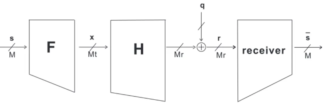
Consider the MIMO system with Mt transmit antennas and Mr receive

an-tennas in Figure 2.1. The channel is modeled by an Mr× Mt memoryless

matrix H with Mr×1 channel noise vector q. We assume the channel is slow

fading so that the channel does not change during each channel use. The noise vector q is assumed to be additive white Gaussian with zero mean, unit variance and E[qq†] = N0IMr. The channel considered in this thesis is

of the form

H = HwR 1/2

t , (2.1)

where Hw is an Mr× Mt matrix whose elements are independent Gaussian

random variables with zero mean and unit variance. The matrix Rt, of

dimensions Mt× Mt, is called the transmit correlation matrix. In this case,

the rows of H are independent and each has autocorrelation matrix equal to

Rt. Let the eigen decomposition of Rt be

Rt = U†tΛtUt,

where Λt is a diagonal matrix and the diagonal elements λt,i are the

eigen-values of Rt. Let the diagonal elements of λt,i be ordered such that λt,0 ≥

Mr M Mt M q r s _ s Mr

H

F

Figure 2.1: The system model of MIMO transmission system.

Suppose the transmitter and receiver can process M substreams of symbols, where M ≤ min(Mt, Mr − 1). The spatial multiplexing precoder F is an

Mt× M matrix with orthonormal columns. The input vector s is an M × 1

vector consisting of modulation symbols sk, for k = 0, 1, . . . , M− 1, carrying

bk bits. The number of bits transmitted per channel use is thus

Rb = M∑−1

k=0

bk.

The symbols sk are assumed to be uncorrelated with zero mean and unit

variance, E[ss†] = IM. The total transmission power is constrained to be Pt.

Thus, we have tr(E[xx†]) = tr(E[Fss†F†]) = tr(FF†)≤ Pt.

2.2

Receiver Design

In this thesis, we will consider two types of zero forcing receivers, linear and decision feedback receivers.

2.2.1

Linear receiver

When the receiver is linear and zero forcing, the receiver is an M×Mrmatrix.

We denote it as G,

G = (F†H†HF)−1F†H†.

[23] The receiver output is s = Gr. Define the error vector at the output of the receiver as e = s− s. In this case, the error vector e has autocorrelation

matrix Re = N0E[ee†] given by [23]

Re = N0(F†H†HF)−1.

We can obtain the kth average subchannel error variance ¯σ2

ek by averaging

the above error covariance matrix over the correlated channel. Let the ith column of Hdag be gi, then the autocorrelation matrix of gi is equal to Rt. It

is known that H†H = ∑M_k=0−1gig†i has a complex Wishart distribution with

Mr degrees of freedom, denoted as WMt(Rt, Mr) [24]. If F is a nonsingular

matrix then the matrix R−1_e = N₀−1F†H†HF has a Wishart distribution

WM(N0−1F†RtF, Mr). It has been shown in [22] that when a matrix C is of

Wishart distributionWp(A, t) with t > p, then E[C−1] = _t−p1 A−1. Using this

result, Re = E[Re] is given by

Re =

N0

Mr− M

(F†RtF)−1, where Mr > M. (2.2)

2.2.2

Decision feedback receiver

M r s′ Mr detector

W

B

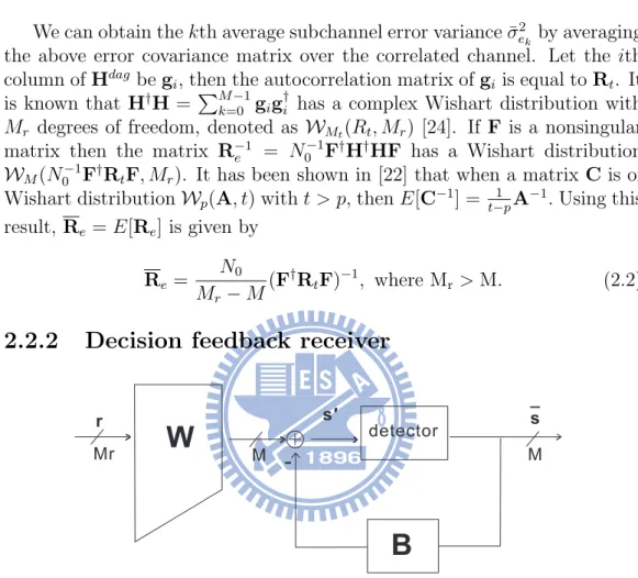
Figure 2.2: Block diagram of the decision feedback receiver based on QR decomposition.

To consider a decision feedback receiver, we can use the receiver structure in Figure 2.2 based on the QR decomposition of HF [33]. This corresponds to the case of a reverse detection ordering which detects from the M th to the 1st subchannel. Let the QR decomposition of HF be QR, where Q is an Mr× M matrix with orthonormal columns and R is an M × M upper

triangular matrix with [R]ii = rii. The feedforward matrix W and feedback

matrix B are given respectively by

W = diag ( r₀₀−1, r₁₁−1, . . . , r_M−1_−1,M−1 ) Q†, B = diag ( r₀₀−1, r₁₁−1, . . . , r_M−1_−1,M−1 ) R− IM.

Assuming there is no error propagation, the kth subchannel error ek =

s′_k− sk has variance σe2k = N0r

−2

kk, for k = 0, 1, . . . , M− 1. The error variance

averaged over the random channel is σ2

ek = E[σ

2

ek] = N0E[r

−2

kk]. The value

E[r_kk−2] has been shown to be related to the Cholesky decomposition of F†RtF

in [33] when Mr > M. Let the Cholesky decomposition of F†RtF be LDL†,

where L is a lower triangular matrix with unity diagonal elements and D is diagonal. Then σ2_e k = N0E[r −2 kk] = N0d−1kk Mr− k − 1 , k = 0, 1, . . . , M − 1, (2.3) where dkk is the kth diagonal element of D.

Bit Error Rate The inputs skare bk-bits QAM symbols, the kth symbol

error rate can be approximate by [47]

SERk= 4(1− 2−bk/2)Q (√ 3 (2bk − 1)σ2 ek ) . (2.4) When gray code is used, then BER can be approximated by BERk ≈

SERk/bk. Then BER≈ 1 Rb M∑−1 k=0 bkBERk ≈ 1 Rb M∑−1 k=0 SERk. (2.5)

Other Detection Orderings

• Forward ordering

Similar to the reverse ordering, the detection order of forward order-ing is fixed but detection starts from the 1st to the M th subchannel.

The receiver structure is similar to that in Figure 2.2 and we use QL decomposition to replace the QR decomposition. Let the QL decompo-sition of HF be QLq, where Q is an Mr× M matrix with orthonormal

columns and Lq is an M×M lower triangular matrix with [Lq]ii= lq,ii.

The feedforward matrix W, feedback matrix B and σ2_e

k in [35] are given by W = Q diag ( l−1_q,00, l_q,11−1 , . . . , l−1_q,M−1M−1 ) , B = diag ( l−1_q,00, l−1_q,11, . . . , l−1_q,M−1M−1 ) L− IM

Let the Cholesky decomposition of F†RtF be L†1D1L1, where L1 is a

lower triangular matrix with unity diagonal elements and D1 is

diago-nal. And the error variance averaged over the random channel is

σ2_e k = N0E[l −2 kk] = N0d−11,kk Mr− M + k + 1 , k = 0, 1, . . . , M − 1, (2.6) where d1,kk is the kth diagonal element of D1.

• VBLAST ordering [14]

In the VBLAST system, the detection ordering is not fixed. It is based on the current channel. The decision feedback receiver can be described as a recursive procedure [14]. First initializes r0 = r, A0 = HF and

i = 0. The steps in the recursions are as follows. (1) Let Gi be the

Moore-Penrose inverse of Ai. Find the row vector of Gi that has the

smallest 2-norm. Call the index of the row vector ni and the row

vector wi. (2) Compute yi = wiri, apply symbol detection on yi, and

call the output sni. (3) Subtract from ri the contribution of the nith

subchannel, ri+1 = ri − sniani, where ani is the nith column of A0,

and zero the nith column of Ai to obtain Ai+1. ρni is maximized in

the nth stage and the post detection SNR of the nith subchannel is

ρni =

Pt

M N0||wi||2, hen all the subchannels are of the same constellation.

In this case, the above procedure is optimal in the sense that the worst subchannel error rate is minimized.

• Rate-Normalized-SNR ordering

that of VBLAST [14]. The only difference is that the rate normalized SNR ρni = Pt M N0(2bni − 1)||wi||2 is maximized. • Greedy QR ordering [15]

The algorithm is proposed in [15] for efficient ordering using QRE de-composition. The recursive procedure starts by minimizing the error variance of last detection layer by a permutation matrix Γ1 and unitary

matrix Q1. Then we repeat the same procedure to find Γ2, . . . , ΓMt

and Q2, . . . , QMt. At last, this ordered QR decomposition of H has

the following form HΓ = QR, where Γ = Γ1Γ2· · · ΓMt is a

permuta-tion matrix, Q = Q1Q2· · · QMt is an unitary matrix with orthonormal

columns and R is an upper triangular matrix. The permutation matrix

Chapter 3

Previous Works of Statistical

Designs

In this chapter, previous works on statistical precoder and bit allocation are reviewed. Section 3.1 recaps the statistical prcoder design with linear zero forcing receiver proposed in [25] and [26]. In section 3.2, we present the method of designing optimal statistical zero forcing decision feedback precoder are proposed in [33] and [35] for equal or given bit allocation. In section 3.3, the designs of statistical bit allocation without precoder were proposed in [40] and [42]. In all sections, full knowledge of channel state information is available at receiver. At the transmitter, however, only statis-tical characteristics of the channel are available.

3.1

Statistical Precoders for Linear Receivers

In this subsection, we review the statistical precoder proposed in [25] for linear zero forcing receiver. In [25], the system model is the same as that in section 2.2.1. The bit allocation is uniform and the target bit rate is a multiple of M . Each symbol carries Rb/M bits. Using the results from [27]

and [28], the average probability of a symbol error Pe,k on subchannel k can

be bounded by Pe,k ≤ β ( N0[(F†RtF)−1]kk )Mr−M+1 ,

where β is a constant depending on the modulation. In order to solve the optimal F that optimizes the cumulative error probability of all subchannels,

the equivalent constrained optimization problem is formulated as minimize F ∑M−1 k=0 ( [(F†RtF)−1]kk )Mr−M+1 subject to tr(FF†) = Pt The optimal statistical precoder is of the form

FKSV R = √ Pt T r(Λ−1/2_t,M )Ut,MΛ −1/4 t,M WM, (3.1)

where WM is a normalized M × M DFT matrix and Ut,M and Λt,M are

respectively submatrices of Ut and Λt consist of the first M columns of Ut

and Λt.

3.2

Statistical Precoders for Decision

Feed-back Receivers

In this subsection, we introduce the statistical precoder design method for zero forcing decision feedback systems that use convex optimization tech-nique. The design method was first proposed in [33] considered equal bit allocation and minimization of MSE. More general method was proposed in [35] that considered different types of objective functions for a given bit allocation. The system in [33] requires M = Mt < Mr and the system in [35]

requires M ≤ min(Mt, Mr− 1).

In [33], the optimal statistical precoder is designed by minimizing the average arithmetic mean-squared error (MSE) subject to a constraint on the total transmission power. The bit allocation here is uniform and the optimization problem shown as follows:

minimize F EH [_∑ Mt−1 k=0 r−2kk ] subject to tr(F†F)≤ Pt,

λt,k and E[rkk−2], the equivalent optimization problem is as follows. minimize dk,pk ∑Mt−1 k=0 1 Mr−k+1e −dk subject to        ∑Mt−1 k=0 epk = Pt p₁ ≥ p₂ ≥ . . . ≥ p_Mt ∑M0−1 k=0 dk ≤ ∑M0−1 k=0 pk+ ∑M0−1 k=1 λt,k, 1≤ M0 < Mt ∑Mt−1 k=0 dk = ∑Mt−1 k=0 pk+ ∑Mt−1 k=0 λk ,

where dk= log dk, pk = log pkand dkis as the same as dkkin (2.3). The above

design problem is called Geometric Programming and is a convex optimiza-tion problem that can be efficiently solved using an interior point method [38]. Let Dp = diag(p 1/2 0 , p 1/2 1 , . . . , p 1/2 Mt−1) and Lg = diag(p0λt,0, p1λt,1, . . . , pMt−1λt,Mt−1).

Let the generalized triangular decomposition [34] of L1/2g be NΓS†, where

N and S are two Mt× Mt matrices with orthonormal columns and Γ is an

upper triangular matrix with diag(Γ) = diag(d0, d1, . . . , dMt−1). The optimal

statistical precoder has the following form

FLZW = UtDpS. (3.2)

In [35], the optimal statistical precoder is designed by minimizing a convex cost function subject to a constraint on the total transmission power. The convex cost function can be the sum of average MSE, average joint error probability and average outage probability function. The bit allocation is not necessarily uniform. The case of is sum of average MSE is reviewed below. The optimization problem is formulated as

minimize ηk,pk ∑M−1 k=0 e−q(ηk−αk ) subject to        ∑M−1 k=0 epk = Pt p₁ ≥ p₂ ≥ . . . ≥ p_M ∑M0−1 k=0 ηk ≤ ∑M0−1 k=0 pk+ ∑M0−1 k=1 λt,k, 1≤ M0 < M ∑M−1 k=0 ηk = ∑M−1 k=0 pk+ ∑M−1 k=0 λt,k

,where q denotes the qth norm of average mean square error, αk= log2

(

2bk₋₁

Mr−M+k−1

) ,

solved by the interior point method [38]. Let e

Λ = diag(p0λt,0, p1λt,1, . . . , pM−1λt,M−1),

diag(R1) = diag(η0, η1, . . . , ηM−1)

and take the generalized triangular decomposition on ( eΛ1/2₎†_{= ZR}

1I†, where

Z and I are two M × M matrices with orthonormal columns and R1 is an

upper triangular matrix. Then the optimal statistical precoder is given by

FJ OJ = Ut,MDpZ. (3.3)

3.3

Statistical Bit Allocation with Decision

Feedback Receiver

In this subsection, we recaps two methods for finding statistical bit alloca-tion in [40] and [42] . In [40], the bits are allocated based on statistics for an i.i.d. channel. In [42], the number of transmit antennas together with the transmit symbol constellations are determined using the knowledge of channel correlation matrices.

3.3.1

Statistical bit allocation for i.i.d. channel

For a flat-fading MIMO channel Hw(Mt ≤ Mr) assumed in (2.1), the

rela-tionship between transmitted symbol s and received symbol r is

r = Hws + q,

where q is the noise vector which has the same definition in Chapter 2. Assuming that each transmit antenna has equal transmit power and forward detection ordering is used, the instantaneous transmission rate to be allocated to transmit antenna l is Cl = log2det(IMr + Pt MtN0 Hl−1H†l−1)− log2det(IMr + Pt MtN0 HlH†l),

where Hl = [hl+1hl+2. . . hMt] and Pt is the total transmission power. It has

been observed that the distribution of the capacity of a MIMO Rayleigh chan-nel can be accurately approximated by a Gaussian distribution at medium

and high SNR [20] [21], denoted as Cl ∼ N(ηl, σl), where ηl and σl are the

mean and variance of the lth transmission rate. In order to select data rates for different antennas, the outage probability of the whole system is mini-mized. It is equivalent to maximizing the probability when no subchannel have transmission rate greater than the respective subchannel capacities and the optimization problem is as follows

minimize bl∈R ∏M t−1 l=0 ∫_∞ bl 1 √ 2σK,le −(t−ηl)2 2σ2 K,l dt subject to ∑M t_l=0−1bl= Rb ,

where σK,l = σl/K, K is the number of independent channel realizations.

Then, the optimum bit allocation for the lth antenna is

bl ≈ ηl+ σl ∑Mt m=1σm (Rb− Mt ∑ m=1 ηm). (3.4)

3.3.2

Statistical bit allocation for correlated channel

In [42], the author proposed a selection criteria to choose the optimal transmit antenna set υ which maximize the minimum subchannel SNR given by

(Mt, υ) = arg max ( fMt,eυ) [ 1 f Mt ( ln det(R_{t( fM} t,eυ)) + f Mt ∑ j=1 M∑r−j i=1 1 i − Rbln 2 ) − ln fMt ] , (3.5) where fMt is the number of active antennas of the transmit antenna set eυ.

After the optimal transmit antenna set υ is chosen, the real bit allocation is derived by assuming post detection SNR are all the same and the statistical bit allocation is obtained by the below equation

bi|Hw = Rb Mt + 2 log|λi(R)| − 1 Mt log₂det(R†R), (3.6) where R is obtained from the QR decomposition of Hw = QR and λi(R)

Chapter 4

Statistical Precoder Design

For a given precoder, we will first derive the statistical BER bound and the optimal real bit allocation. Based on the BER bounds, we can obtain the optimal precoder under the transmission power constraint. At last, we will discuss methods for finding statistical integer bit allocation.

4.1

Derivation of Statistical BER Bound and

Optimal Real Bit Allocation

The BER can be computed using (2.4) and (2.5). For the convenience of derivation, we define the function

f (y) = Q(1/√y), y > 0.

The function f (y) is monotone increasing and it can be verified that f (y) is convex for y ≤ 1/3 and concave for y ≥ 1/3.

High SNR case Let us consider the high SNR case in which the

con-vexity of f (.) holds. Using f (.), we have SERk = 4(1− _2bk/21 )f

( (2bk_−1)σ2 ek 3 ) and BER = _R4 b ∑M−1 k=0 (1− 1 2bk/2)f ( (2bk_−1)σ2 ek 3 )

E[BER]≈ 1 Rb M∑−1 k=0 4(1− 1 2bk/2)E[f ( (2bk− 1)σ2 ek 3 ) ] (4.1) ≥ 4 Rb M∑−1 k=0 (1− 1 2bk/2)f ( (2bk− 1)¯σ2 ek 3 ) (4.2) , ϕM(b), (4.3)

where b = [b0 b1. . . bM−1] is the bit allocation vector. The inequality in (4.1)

is obtained using Jensen’s inequality. Assume bk is large enough so that

(1− 2−bk/2₎≈ 1 and 2bk − 1 ≈ 2bk_{, then} ϕM(b)≈ 4 Rb M∑−1 k=0 f (2 bk_σ¯2 ek 3 ) ≥ 4 Rb/M f ( 1 M M∑−1 k=0 ( 2bk_σ¯2 ek 3 )) (4.4) ≥ 4 Rb/M f ( 1 3 (M∏−1 k=0 2bk_σ¯2 ek )1/M) (4.5) = 4 Rb/M f ( 2Rb/M 3 (M∏−1 k=0 ¯ σ_e2 k )1/M) , ΩM.

The inequality in (4.4) is due to the convexity of f (.). The inequality in (4.5) is due to AM-GM (arithmetic mean-geometric mean) inequality and the monotone increasing property of f (.). Due to the convexity of f (.), the inequality in (4.4) holds if and only if 2bk_σ¯2

ek are of the same value for all k

and ∑M_k=0−1bk= Rb. The optimal bit allocation for minimizing ϕM(b) is thus

bk= Rb M − log2(¯σ 2 ek) + 1 M M∑−1 j=0 log₂(¯σ_e2_j), k = 0, 1, . . . , M− 1. (4.6) For convenience, we call the above optimal real bit allocation as breal,M.

Low SNR case Using a similar procedure, we can derive the statistical

BER bound for the low SNR case in which the concavity of f (.) holds.

E[BER]≤ 4 Rb M∑−1 k=0 (1− 1 2bk/2)f ( (2bk− 1)¯σ2 ek 3 ) = ϕM(b) (4.7)

In this case, ϕM(b) is an upper bound of averaged BER. Assume as in the

high SNR case that each subchannel transmission rate bk is high enough so

that (1− 2−bk/2₎≈ 1 and 2bk − 1 ≈ 2bk_{, then}

ϕM(b)≈ 4 Rb M∑−1 k=0 f ( 2bk_σ¯2 ek 3 ) ≥ 4 Rb/M f ( 1 M M∑−1 k=0 (2 bk_σ¯2 ek 3 ) ) = ΩM. (4.8)

That is ϕM(b) has minimum equal to ΩM. The minimum achieved when

bit allocation is as given in (4.6). In this case, the equality in (4.8) becomes an equality and we have ϕM(b) ≈ ΩM as in the high SNR case. Therefore

ΩM is a lower bound of averaged BER in the high SNR case and a upper

bound in the low SNR case. For both high and low SNR cases, we would like to have the bound ϕM(b) minimized. The minimization of the lower bound

in high SNR case is also important because the averaged BER can not be small if the lower bound is large.

4.2

Precoder Design

Our goal now is to find the optimum precoder =F that to minimize ΩM.

This optimization problem is as follows: minimize F f ( 2Rb/M 3 (M∏−1 k=0 ¯ σ_e2 k )1/M) (4.9) subject to T r(F†F)≤ Pt.

• Decision feedback receiver:

Since f (.) is a monotone increasing function, minimizing (4.9) is equiv-alent to minimizing (∏M_k=0−1σ¯2

ek)

1/M_{. Here, we will find the precoder F}

which minimizes (∏M_k=0−1σ¯2 ek)

Using (2.3), we have∏M_k=0−1σ¯2 ek = ∏M−1 k=0 N0d−1_kk Mr−k−1. Note that ∏M−1 k=0 d−1kk =

det(F†RtF). Let the singular decomposition of F be

F = UfΣfV†_f,

where Uf is Mt× M with U†fUf = IM, Vf is M × M unitary with

V_f†Vf = IM and Σf is an M × M diagonal matrix. Then

det(F†RtF) = det(Σf) det(U†_fRtUf).

It follows that M∏−1 k=0 ¯ σ_e2 k = 1 det(F†RtF) M∏−1 k=0 N0 (Mr− k − 1) = 1 det(Σf) det(U†_fRtUf) M∏−1 k=0 N0 (Mr− k − 1).

As Uf has orthonormal columns, we can apply the Poincare

separa-tion theorem [43] to bound det(U†_fRtUf) using the eigenvalues of Rt.

Poincare separation theorem says λi(B)≥ λi(C†BC), i = 0, 1, . . . , r−

1, for any n× n Hermitian matrix B and any n × r unitary matrix C with C†C = Ir. Using this theorem, we have

det(U†_fRtUf)≤ M∏−1

i=0

λt,i.

On the other hand det(Σ2_f) = M∏−1 i=0 [Σ2_f]ii≤ ( tr(Σ2_f)/M )M = ( tr(F†F)/M )M ≤ (Pt/M )M. Thus det(F†RtF) ≤ (Pt/M )M ∏M−1

i=0 λt,i and the product of averaged

error variance satisfies

M−1_∏ k=0 ¯ σ_e2 k ≥ 1 det(Σf) M∏−1 k=0 N0 λt,i(Mr− k − 1) ≥ M−1_∏ k=0 M N0 Ptλt,i(Mr− k − 1) . (4.10)

Because the choice of unitary matrix Vf does not effect the value

det(F†RtF), we choose Vf = IM without loss of generality. The

equal-ity (4.10) holds if F = Ut,M and the diagonal element of Σf are

iden-tical. Therefore the optimal precoder

F =

√

Pt

MUt,M. (4.11) • Linear receiver:

From [36], we know an increasing function of a Schur-concave function is Schur-concave. Because (∏M_k=0−1σ¯2

ek)

1/M _{is a Schur-concave function and}

f (.) is monotone increasing function, the objective function in (4.9) is

concave. Using the result of [29], the optimal precoder for Schur-concave objective function under total transmission power constraint has the form Fop = Ut,MΣp, where Ut,M ∈ CMt×M has as columns

the eigenvectors of Rt corresponding to the M largest eigenvalues in

decreasing order and Σp = diag(p1, p2, . . . , pM)∈ CM×M. In this case,

the product of the averaged error variance is given by

M∏−1 k=0 ¯ σ2_ek = ( N0 Mr− M )M M−1_∏ k=0 λ−1_t,k M∏−1 k=0 p−2_k (4.12) Furthermore the constraint in (4.9) can be simplified as follows:

T r(F†_opFop) = T r(Σ†pU†t,MUt,MΣp) = M∑−1

k=0

p2_k≤ Pt.

Since f (.) is a monotone increasing function, minimizing (4.9) is equiv-alent to minimizing (∏M_k=0−1σ¯_e2_k)1/M, which, due to (4.12), is equivalent to minimizing ∏M_k=0−1p−2_k . The original problem can be reduced to the equivalent one shown below.

minimize pk M∏−1 k=0 p−2_k subject to M∑−1 k=0 p2_k≤ Pt.

By using AM-GM inequality, the above problem can be solved easily and the optimal power allocation is pk=

√

Pt

M, k = 1, 2, . . . , M .

There-fore we obtain the optimal precoder as

Fopt =

√

Pt

MUt,M,

which is the same as the optimal precoder for the decision feedback receiver.

4.3

Design of Integer Bit Allocation

The optimal bit allocation compared in (4.6) has real entries. In prac-tical applications, bk should be nonnegative integers. In this section, we

will present methods for designing integer bit allocation with given precoder

F =

√

Pt

MUt,M. First, we will introduce two numerical methods of integer bit

allocation design. Second, we will present two methods based on the statisti-cal BER bound. At last, we will consider the optimal number of subchannel used. The methods given in this section can be applied for both linear and decision feedback receiver. All bit allocations discussed here have positive entries.

4.3.1

Minimum BER bit allocation (b

)

We denoteCb,M as a bit allocation codebook which contains all length equal to

or less than M positive integer bit allocation vectors such that∑M_k=0−1bk = Rb.

For each bit allocation in codebookCb,M, we calculate its corresponding

aver-age BER performance using a large number of random channels. The vector that has the smallest average BER performance is denoted as bmber and it

represents the best bit allocation in BER performance.

4.3.2

Most probable bit allocation (b

)

First, we generate a large number of training channels. For each training channel, we can find the corresponding BER-minimizing bit allocation vector in Cb,M. The vector bprob is the most probable bit allocation.

4.3.3

Bit allocation using greedy algorithm (b

)

When the transmission power Pt is large enough so that all argument of f (.)

in ϕM(b) are smaller than 1/3 and f (.) is operating at the convex region. We

can use the greedy algorithm to solve this allocation problem efficiently. The solution of this kind of optimization problem was first proposed in [44]. This algorithm is also called ”marginal allocation” or ”incremental” algorithm. More detailed analysis was proposed in [45].

In [45], the allocation problem has the following form. minimize xk∈{0,1,...,M} ∑M−1 k=0 Fk(xk) subject to ∑M−1_k=0 xk = N ,

where N is a positive integer and the function Fk(.) is convex in xk.

The optimal x is determined as follows.

• Step 1 Let x = (0, 0, . . . , 0) be a M × 1 vector and r = 0. • Step 2 Let v = arg min j∈{0,1,...,M} ( Fj(xj + 1)− Fj(xj) ) , then xv = xv+ 1.

• Step 3 If r = N, then stop. The current x is an optimal solution.

Otherwise, r = r + 1 and return to step 2. Ignoring the factor (1−2−bk/2_{), then ϕ}

M(b) in (4.3) can be approximated as ϕM(b) = 4 Rb M∑−1 k=0 Fk(bk), where Fk(bk) = f ( (2bk_−1)¯σ2 e,k 3 )

. Suppose SNR is high so that the argument

in f (.) is smaller than 1/3. In this case, Fk(bk) is convex and the greedy

Remark In Section 4.1, we have obtained a optimal real bit allocation breal,M. Then we can use the quantization method referred in [46] to get a

positive integer bit allocation denoted as bi,M. Because breal,M is also derived

by the convex assumption, bi,M is the same as bgr,M in our simulations.

4.3.4

Bit allocation for minimizing statistical bound

(b

)

Here, we introduce the statistical integer bit allocation that minimizes ϕM(b).

We denote this statistical bit allocation as bd,M and is given by

bd,M = arg min_{b ∈ C}

b,M ϕM(b). (4.13)

The vector bd,M can be obtained by an exhausted search. In Section 4.3.2,

we have shown greedy integer bit allocation is also optimal so these two statistical integer bit allocations are the same in high SNR region. However, if the arguments of f (.) for the optimal bit allocation are not all located at convex or concave region, then the optimal bit allocation can not be found by the greedy algorithm. In the simulations, the performance of bd,M is very

close to that of bmber. It can be used for all SNR region.

4.3.5

Optimal number of substream M

The optimal precoder derived in Sec 4.2 is F = √

Pt

MUt,M, which is obtained

under the high bit rate assumption bk ≫ 1. Implicity M substreams are

transmitted. We can also consider the transmission of fewer substreams. Let

M0 be the number of substreams transmitted. When we reduce M0, each

subchannel will be allocated more transmission power but more bits. Con-versely, each subchannel is allocated less transmission power but fewer bits when we choose larger M0. The tradeoff between different M0has become an

interesting issue. Recently, there are several researchers (e.g. [42], [48], [49] and [50]) mentioned that wireless MIMO system could have better perfor-mance when the number of subchannels used is variable. In these papers, the

M0 selection function plays an important role on system performance. Here,

we choose ϕM0(b) we have derived earlier as our selection function. We can

find the best bit allocation to minimize ϕM(b) for each M0 and choose the

• Step 1 For each M0 ∈ {1, 2, . . . , M}, the corresponding optimal

pre-coder is F = √

Pt

M0Ut,M0. Then we apply the greedy algorithm in Sec

4.3.3. to find bgr,M0 such that the statistical BER bound ϕM0(bgr,M0)

in (4.3) is minimized.

• Step 2 The optimum number of substreams is given by

Mopt = _{i∈{1,2,...,M}}arg min ϕi(bgr,i). (4.14)

and the corresponding optimal bit allocation is bgr,Mopt.

In a similar manner, we can obtain the bd,M0 for each M0 ∈ {1, 2, . . . , M}.

Then we can also use ϕM0(b) as the selection function to find the best integer

Chapter 5

Simulation Result

In this chapter, we present simulation results of our statistical precoder and statistical bit allocation (staP-BA) system. In our simulations, we use the exponential model for the channel correlation matrix Rt. A 4×4 example of

Rt is given below Rt=     1 ρ ρ2 _ρ3 ρ∗ 1 ρ ρ2 ρ∗2 ρ∗ 1 ρ ρ∗3 ρ∗2 ρ∗ 1     ,

where ρ∗ denotes the complex conjugate of ρ. We denote the uniform bit allocation as buni. In all examples, bprob and bmber are found at the high

SNR region using 105 training channels. We have used 106 channels in the simulation examples.

Example 1. Comparison of different integer bit allocation schemes.

In this example, we discuss the BER performance between different statisti-cal bit allocation methods proposed in Chapter 4 and we use the proposed precoder F =

√

Pt

MUt,M and reverse ordering detected from the M th to the

1st substream.

A. For Mr = 4, Mt = 3, M = 3, Rb = 12, we show BER plots for

different ρ in Figure 5.1. We can see bgr,Mopt is the same as bd,Mopt and bmber

for the different correlation parameters. Also shown is the statistical BER bound ϕMopt(bgr,Mopt) a lower bound in high SNR region and an upper bound

(a) 10 15 20 25 30 35 40 10−5 10−4 10−3 10−2 10−1 P t/N0 BER b prob=(4 4 4) b

mber=bgr,Mopt=bd,Mopt=(5 4 3)

φ_Mopt(b gr,Mopt) (b) 10 15 20 25 30 35 40 10−5 10−4 10−3 10−2 10−1 P t/N0 BER b

prob=bmber=bgr,Mopt=bd,Mopt=(6 4 2)

φ_Mopt(b

(c) 15 20 25 30 35 40 10−5 10−4 10−3 10−2 10−1 P t/N0 BER b

prob=bmber=bgr,Mopt=bd,Mopt=(8 4)

φ_Mopt(b

gr,Mopt)

Figure 5.1: Example 1.A. Different Integer Bit Allocation schemes (Mr =

B. For Mr = 6, Mt = 4, M = 4, Rb = 8, we can see the BER plots

in Figure 5.2. bgr,Mopt is still the same as bd,Mopt and bmber for different

correlation parameters. This corroborate our earlier observation that when the transmission power is high enough so that all f (.) is operating at convex region, bd,Mopt and bgr,Mopt should be the same. Figure 5.1 and 5.2 confirm

this conclusion. (a) 10 15 20 25 30 10−6 10−5 10−4 10−3 10−2 10−1 P t/N0 BER b prob=(2 2 2 2) b mber=bgr,M opt =b d,Mopt=(3 3 2) φ_Mopt(b gr,Mopt)

(b) 10 15 20 25 30 10−6 10−5 10−4 10−3 10−2 10−1 P t/N0 BER b

mber=bprob=bgr,Mopt=bd,Mopt=(3 3 2)

φ_Mopt(b gr,Mopt) (c) 10 15 20 25 30 10−6 10−5 10−4 10−3 10−2 10−1 P t/N0 BER b

mber=bprob=bgr,Mopt=bd,Mopt=(5 3)

φ_Mopt(b

gr,Mopt)

Figure 5.2: Example 1.B. Different Integer Bit Allocation schemes (Mr =

Example 2. Performance for different Vf. In this example, we

dis-cuss the BER performance between different Vf chosen in section 4.2. The

parameter settings are Mr = 6, Mt = 4, M = 4, Rb = 18. The proposed

precoder is F = √

Pt

MUt,MVf and the reverse ordering is used. Five different

Vf are used

• √Pt

MIM t,M.

• DFT matrix. • DCT matrix.

• Random unitary matrix. • √Pt

MU′t,M.

For each Vf, the corresponding breal,M and bgr,M can be found in Section 4.1

and 4.3.3. The BER performances and ϕM(b) are shown in Figure 5.3. In

Figure 5.3 (a), we can find there are only a little difference between different

Vf. In Figure 5.3 (b), the BER difference become smaller when breal,M

is used. Now we assume bk is large enough so that (1 − 2−bk/2) ≈ 1 and

2bk−1 ≈ 2bk_{, then the BER formula used in (2.5) for simulations is turned to}

be BER ≈ _R4 b ∑M−1 k=0 f ( 2bkσ2 ek 3 )

. The result is shown in Figure 5.3 (c). We

can find the BER performance between different Vf are all the same. For

convenience, we will all use Vf =

√

Pt

(a) 18 20 22 24 26 28 30 10−6 10−5 10−4 10−3 10−2 10−1 P t/N0 BER Ide, (7 5 4 2) DFT, (6 5 4 3) DCT, (6 4 4 4) Random, (5 5 4 4) Ut, (6 4 4 4) Ide, φ 4(7 5 4 2) DFT, φ 4(6 5 4 3) DCT, φ 4(6 4 4 4) Random, φ 4(5 5 4 4) Ut, φ 4(6 4 4 4) (b) 18 20 22 24 26 28 30 10−5 10−4 10−3 10−2 10−1 P t/N0 BER Ide, (7.2699 5.0947 3.4348 2.2007) DFT, (5.8238 4.8099 4.1520 3.2143) DCT, (5.9579 4.3728 4.0189 3.6504) Random, (5.3322 4.7385 4.1361 3.7932) Ut, (5.8238 4.5304 4.1154 3.5304)

(c) 18 20 22 24 26 28 30 10−5 10−4 10−3 10−2 10−1 P t/N0 BER Ide, (7.2699 5.0947 3.4348 2.2007) DFT, (5.8238 4.8099 4.1520 3.2143) DCT, (5.9579 4.3728 4.0189 3.6504) Random, (5.3322 4.7385 4.1361 3.7932) Ut, (5.8238 4.5304 4.1154 3.5304)

Figure 5.3: Example 2.A. Performance for different Vf (Mr = 6, Mt =

4, M = 4, Rb = 18) for (a) bgr,4, (b) breal,4 and (c) breal,4 with high bit rate

Example 3. Performance for different M0. In this example, the

pre-coder used is F = √

Pt

MUt,M. For a given M0, we find the optimal integer bit

allocation that minimizes ϕM0(b) using the greedy algorithm in Sec 4.3.3. By

calculating ϕM0(b) for each M0, we obtain the optimal number of substream

Mopt which has minimum ϕM0(b) in Sec 4.3.5.

A. For Mr = 4, Mt = 3, M = 3, Rb = 12, the BER plots are shown

in Figure 5.4. In this case, Mopt is 3 for ρ = 0, 0.5. We can see in Figure

5.4 (a) (b), the use of 3 substreams given a better performance for both reverse ordering. For ρ = 0.9, the optimal number of substream Mopt is 2

and Figure 5.4 (c) shows that using 2 substreams yields a lower error rate. This demonstrates that the statistical lower bound ϕM0(b) provides a useful

reference. (a) 10 15 20 25 30 35 40 10−5 10−4 10−3 10−2 10−1 P t/N0 BER b gr,3=(5 4 3) b gr,2=(6 6) φ₃(b gr,3) φ₂(b gr,2)

(b) 10 15 20 25 30 35 40 10−5 10−4 10−3 10−2 10−1 P t/N0 BER b gr,3=(6 4 2) b_gr,2=(7 5) φ₃(b_gr,3) φ₂(b_gr,2) (c) 15 20 25 30 35 40 10−5 10−4 10−3 10−2 10−1 P t/N0 BER b_gr,3=(8 3 1) b gr,2=(8 4) φ₃(b gr,3) φ₂(b gr,2)

Figure 5.4: Example 3.A. Performance for different M0 (Mr = 4, Mt =

3, M = 3, Rb = 12) for (a) ρ = 0, Mopt = 3, (b) ρ = 0.5, Mopt = 3 and (c)

B. For Mr = 6, Mt= 4, M = 4, Rb = 8, the BER performance is shown

in Figure 5.5, Mopt is 3 for ρ = 0, 0.3 and Moptis 2 for ρ = 0.7. Again, we can

see that using the statistical bound ϕM0(b) is a useful reference to determine

the number of substreams transmitted.

(a) 10 15 20 25 30 10−6 10−5 10−4 10−3 10−2 10−1 P t/N0 BER b gr,4= (3 2 2 1) b gr,3= (3 3 2) b gr,2= (4 4) b gr,1= (8) φ₄(b gr,4) φ₃(b gr,3) φ 2(bgr,2) φ₁(b gr,1)

(b) 10 15 20 25 30 10−6 10−5 10−4 10−3 10−2 10−1 P t/N0 BER b gr,4= (3 2 2 1) b gr,3= (3 3 2) b_gr,2= (4 4) b_gr,1= (8) φ₄(b gr,4) φ₃(b gr,3) φ₂(b gr,2) φ₁(b gr,1) (c) 10 15 20 25 30 10−6 10−5 10−4 10−3 10−2 10−1 P t/N0 BER b gr,4= (4 2 1 1) b gr,3= (5 2 1) b gr,2= (5 3) b gr,1= (8) φ 4(bgr,4) φ₃(b gr,3) φ₂(b gr,2) φ₁(b gr,1)

Figure 5.5: Example 3.B. Performance for different M0 (Mr = 6, Mt =

4, M = 4, Rb = 8) for (a) ρ = 0, Mopt = 3, (b) ρ = 0.3, Mopt = 3 and (c)

Example 4. Different Precoders. In this example, we compare the performance between different precoders for the same bit allocation and fixed detection ordering. The parameter settings are Mr = 4, Mt = 3, M =

3, Rb = 18. Four different precoders are used

• √Pt

MUt, the precoder given in (4.11) for minimizing the BER statistical

bound.

• FJ OJ, the optimal statistical precoder derived in [35] for a given bit

allocation.

• FLZW, the MSE-minimizing statistical precoder given in [33] for

uni-form bit allocation.

• √Pt

MIMt,M, which consist of first M columns of IMt.

Reverse ordering is used for all precoders except FJ OJ, for which forward

ordering is applied as FJ OJ is designed for forward ordering. We show the

results for two different bit allocation, uniform bit allocation in Figure 5.6 and

bgr,M in Figure 5.7. The vector bgr,M is computed using the greedy algorithm

in Sec 4.3.3. when the precoder is √

Pt

MUt. We can see that for uniform bit

allocation, FJ OJ and FLZW are better than the other two. As correlation

parameter ρ increases, the optimal bit allocation become more nonuniform and FLZW does not perform as well. This is because FLZW is designed for

uniform bit allocation. Notice that FJ OJ performs better because its design

(a) 15 20 25 30 35 40 45 10−5 10−4 10−3 10−2 10−1 P t/N0 BER U t F JOJ F LZW I Mt (b) 15 20 25 30 35 40 45 10−5 10−4 10−3 10−2 10−1 P t/N0 BER U t F JOJ F LZW I Mt

Figure 5.6: Example 4.A. Performance of different precoders for uniform bit allocation. (a) ρ =0.5; (b) ρ =0.9.

When the bit allocation is bgr,M in Fig 5.7, the precoder

√

Pt

MUt become

the best of the four.

(a) 15 20 25 30 35 40 45 10−5 10−4 10−3 10−2 10−1 P t/N0 BER U t F JOJ F LZW I Mt

(b) 15 20 25 30 35 40 45 10−5 10−4 10−3 10−2 10−1 P t/N0 BER U t F JOJ F LZW I Mt

Figure 5.7: Example 4.B. Performance of different precoders when the bit allocation is bgr,M. (a) ρ =0.5, bgr,M = [8 6 4]; (b) ρ =0.9, bgr,M = [10 5 3].

Example 5. Performance for different ρ. In this example, we compare

our staP-BA system with the original system for different ρ. The parameter settings are Mr = 6, Mt = 4, M = 4. The original system is assumed

without precoding (F = IMt) and uniform bit allocation. The results are

shown in Figure 5.8 and 5.9. In Figure 5.8, the BER performance become closer after applying our method. In Figure 5.9, we define the improvement gain as the SNR difference between these two system. Then we can find the improvement gain becomes larger when ρ increases. This demonstrates our staP-BA system has better improvement for highly correlated channels.

(a) 10 15 20 25 30 35 10−5 10−4 10−3 10−2 10−1 P t/N0 BER ρ=0, original ρ=0.3, original ρ=0.5, original ρ=0.7, original ρ=0.9, original ρ=0, staP−BA ρ=0.3, staP−BA ρ=0.5, staP−BA ρ=0.7, staP−BA ρ=0.9, staP−BA (b) 10 15 20 25 30 35 40 10−5 10−4 10−3 10−2 10−1 P t/N0 BER ρ=0, original ρ=0.3, original ρ=0.5, original ρ=0.7, original ρ=0.9, original ρ=0, staP−BA ρ=0.3, staP−BA ρ=0.5, staP−BA ρ=0.7, staP−BA ρ=0.9, staP−BA

Figure 5.8: Example 5.A. Performance for different ρ (Mr = 6, Mt= 4, M =

(a) 0 0.1 0.2 0.3 0.4 0.5 0.6 0.7 0.8 0 5 10 15 ρ Improvement Gain (dB) BER=10−2 BER=10−3 BER=10−4 (b) 0 0.1 0.2 0.3 0.4 0.5 0.6 0.7 0.8 0 2 4 6 8 10 12 ρ Improvement Gain (dB) BER=10−2 BER=10−3 BER=10−4

Figure 5.9: Example 5.B. Comparison of improvement gain (Mr = 6, Mt=

Example 6. Comparison of Different Detection Ordering. In this

example, we use the precoder F = √

Pt

MUt,M and compare the performance

of different detection orderings for the same bit allocation (uniform bit allo-cation or bgr,Mopt). The detection orderings considered are

• Reverse ordering • VBLAST ordering [14] • Greedy QR ordering [15] • Rate-normalized-SNR ordering

• Optimal ordering, which is obtained by an exhausted search of all

de-tection orderings for minimum BER.

A. Mr = 4, Mt = 3, M = 3, Rb = 18, ρ = 0.5. The BER plots

are given for uniform bit allocation is in Figure 5.10 (a) and for bgr,Mopt in

Figure 5.10 (b). For uniform bit allocation, rate-normalized-SNR ordering and VBLAST ordering are the same and the performance is indistinguishable form the optimal ordering. The greedy QR ordering is slightly worse. The selection criteria of greedy QR ordering is minimizing the error variance of the last detected symbol for each recursive procedure and is different from the VBLAST ordering. The reverse ordering has the worst performance because it is a fixed detection ordering. We can not change the detection order to improve the error rate when a subchannel has low SNR.

When bgr,Mopt is used. We see in Figure 5.10 (b) that the BER

perfor-mance of rate-normalized-SNR ordering is very close to the optimal ordering but the VBLAST ordering is not. This demonstrates the importance of tak-ing bit allocation into consideration in determintak-ing detection ordertak-ing when nonuniform bit allocation is used. In this case, reverse ordering performs better than VBLAST and greedy QR ordering because bgr,Mopt is designed

(a) 15 20 25 30 35 40 45 10−5 10−4 10−3 10−2 10−1 P t/N0 BER Reverse VBLAST [14] Greedy QR [15] Rate−n−snr Optimal (b) 15 20 25 30 35 40 45 10−5 10−4 10−3 10−2 10−1 P t/N0 BER Reverse VBLAST [14] Greedy QR [15] Rate−n−snr Optimal

Figure 5.10: Example 6.A. Comparison of different detection orderings for (Mr = 4, Mt= 3, M = 3, Rb = 18, ρ = 0.5) (a) uniform bit allocation, and

B. Mr = 6, Mt = 4, M = 4, Rb = 8, ρ = 0. The BER plot is

given in Figure 5.11. For uniform bit allocation in Figure 5.11 (a), rate-normalized-SNR and VBLAST ordering are the same and the performance is indistinguishable for the optimal ordering. The greedy QR and reverse or-dering performs worse. For bgr,Mopt in Figure 5.11 (b), the BER performance

of Rate-normalized-SNR ordering is also very close to the optimal ordering. Comparing with the previous case in Figure 5.10 (b), the optimal bit alloca-tion bgr,Mopt is more uniform. The VBLAST ordering has less performance

loss. In this case, reverse ordering performs better than greedy QR ordering.

(a) 6 8 10 12 14 16 18 20 22 24 10−6 10−5 10−4 10−3 10−2 10−1 P t/N0 BER Reverse VBLAST [14] Greedy QR [15] Rate−n−snr Optimal

(b) 6 8 10 12 14 16 18 20 22 24 10−6 10−5 10−4 10−3 10−2 10−1 P t/N0 BER Reverse VBLAST [14] Greedy QR [15] Rate−n−snr Optimal

Figure 5.11: Example 6.B. Comparison of different detection ordering (Mr=

6, Mt = 4, M = 4, Rb = 8, ρ = 0) for (a) uniform bit allocation, and (b)

bgr,Mopt = [3 3 2].

Example 7. Comparison with other related works. In this example,

we compare our proposed staP-BA system with the methods reviewed in Chapter 3. The following is a list of systems in the comparison.

• Vertical Bell Laboratories Layered Space-Time (V-BLAST) system [14].

It is a novel Multi-Input Multi-Output (MIMO) antenna scheme and it focuses on the detection algorithms.

• Statistical bit allocation system (staBADu) (reviewed in Sec 3.3.1). It

is designed by minimizing the outage probability error [40]. The in-teger bit allocation used is obtained quantizing the bit allocation in (3.4). The quantization method used is introduced in [46]. The reverse ordering is used in staBADu.

• Statistical bit allocation system (staBARavi) (reviewed in Sec 3.3.2).

It designed by selecting the optimal antenna set [42]. The integer bit allocation used is rounding the bit allocation in (3.6) The greedy QR