國
立
交
通
大
學
資訊科學與工程研究所
碩
士
論
文
利用 GPS 探偵車回報高速公路壅塞路段之系統設計
The
Design of Traffic Report System for Highway Congestions
with GPS-equipped Probe Cars
研 究 生:魏睦倫
指導教授:張明峰 教授
利用 GPS 探偵車回報高速公路壅塞路段之系統設計
The Design of Traffic Report System for Highway Congestions with
GPS-equipped Probe Cars
研 究 生:魏睦倫 Student:Mu-Len Wei
指導教授:張明峰 Advisor:Ming-Feng Chang
國 立 交 通 大 學
資 訊 科 學 與 工 程 研 究 所
碩 士 論 文
A ThesisSubmitted to Institute of Computer Science and Engineering College of Computer Science
National Chiao Tung University in partial Fulfillment of the Requirements
for the Degree of Master
in
Computer Science
June 2012
Hsinchu, Taiwan, Republic of China
i
利用 GPS 探偵車回報高速公路壅塞路段之系統設計
學生:魏睦倫
指導教授:張明峰教授
國立交通大學資訊科學與工程研究所
摘要
提供用路人即時交通資訊,包含車速、車流量等資訊,可節省行車時間及能 源消耗。由於具備各式感測器與無線資料傳輸的智慧型手機逐漸普及,利用在行 駛車輛上的智慧型手機回報取得即時交通資訊成為可行的方式。傳統是利用探針 車傳送旅行資訊,包括車速、車輛位置至交通資訊中心。然而,當探針車數量增 加食,將有許多不必要的資訊回傳至交通資訊中心,增加通訊成本。本研究提出 一個交通回報系統和監測高速公路上塞車狀況。交通資訊中心保存路段上塞車路 段,包括塞車起始結束位置、所需旅行時間,並透過無線網路廣播給路上所有車 輛。當探針車收到資訊後,比對收到廣播訊息和當前旅行路況變化。當兩者在塞 車起始結束位置或旅行時間有巨大變化,探針車將此變化回報給交通資訊中心。 依據這些回報,交通資訊中心更新其保存之資料,並且將這變化廣播告知用路人。 為了分析系統效能,我們使用運輸模擬軟體 VISSIM 來進行實驗模擬。研究成果 證實,我們所提出的方法能有效的偵測高速公路上塞車路段的變化,並且提前警 告 85%以上用路人即將在 100 公尺內遇到塞車。除此之外,此回報機制減少了超 過 50%的探針車和交通資訊中心間之通訊成本。ii
The Design of Traffic Report System for Highway Congestion with
GPS-equipped Probe Cars
Student: Mu-Len Wei
Advisor: Prof. Ming-Feng Chang
Institute of Computer Science and Engineering
National Chiao Tung University
Abstract
Providing real-time traffic information, such as traffic speed and travel time, to road users can save traveling time and reduce fuel consumption. With the increasing popularity of smartphones, which are embedded with a variety of sensors and capable of wireless data communication, smartphones on moving vehicles can be used as probes to collect real-time traffic information. Conventional probe vehicles send their traveling data including speed and location to a traffic information center (TIC) periodically. However, as the number of probes increases, there may be redundant reports sent to the TIC. In this thesis, we present a traffic report system and method to monitor the dynamic changes of traffic jams on highway. The TIC maintains the start location, end location and travel time of each traffic jam, and broadcasts the
information to the probes, as well as the general road users. As the probes travel on the highway, they compare the broadcast traffic jams with their traveling data. If there are significant changes of the start location, end location or travel time are detected, the probes report the changes to the TIC. Based on the reports, the TIC updates the status of traffic jams and broadcasts the new traffic jam information. To evaluate the
performance of our system, we have performed simulations using traffic model simulator VISSIM. The simulation results indicate that our approach can effective monitor the dynamic changes of traffic jams on highway and provides advance warning of traffic jams to over 85% of road users with location errors under 100 m. In addition, the report policy we proposed reduces over 50% of the communication between the probes and the TIC.
iii
誌謝
首先我要感謝指導教授 張明峰老師。就讀研究所期間,老師的指導使我獲 益匪淺。這兩年來,老師悉心指導,讓我學到了做研究的方法。在構思、撰寫此 論文期間,老師也很有耐心地指點論文不足的地方,使我得以完成碩士論文。感 謝老師兩年來的指導。 再來也要謝謝實驗室的同學們,感謝你們在課業以及生活上的幫助,使我得 以順利完成研究所學業。感謝有你們的陪伴,使我生活多采多姿。另外,還要特 別感謝兩位朋友:陳亭方和黃聖翔,在我低潮的時候幫我打氣,並且勉勵一起往 前邁進,感謝你們的支持,才能讓我順利的走完這個階段。 最後,最感謝的是我摯愛的家人。感謝你們的支持,讓我順利完成學業。 魏睦倫 謹識於 國立交通大學資訊科學與工程研究所碩士班 中華民國 101 年 7 月iv
Contents
摘要... i Abstract ... ii 誌謝... iii Contents ... iv List of Figures ... v List of Tables ... vi Chpter 1 Introduction ... 1 1.1 Current Development ... 1 1.2 Motivation ... 2 1.3 Objective ... 3 1.4 Summary ... 4Chpter 2 Background and Related Work ... 5
2.1 FCD-based Traffic Information Systems... 5
2.2 Sensors Embedded in Smartphones Used in Traffic Monitoring ... 6
2.2.1 Global Position System(GPS) ... 7
2.2.2 Gyroscope ... 8
2.2.3 Accelerometer ... 8
2.3 Broadcast Mechanism ... 9
2.4 The Properties of Traffic Jam ... 10
2.5 VISSIM ... 11
Chpter 3 The System Design ... 12
3.1 System Overview ... 12
3.2 Traffic Information Center ... 14
3.3 Probe Cars ... 15
Chpter 4 Evaluation and Analysis ... 20
4.1 Simulation Environment and Parameters ... 20
4.2 Performance Evaluation ... 21
4.2.1 A Single-Lane Freeway with an Interchange Model ... 21
4.2.2 Multi-Lane Freeway with an Interchange Model ... 27
4.2.3 Single-Lane Freeway with a Tollgate Model ... 31
Chpter 5 Conclusions ... 36
v
List of Figures
Fig. 2-1 Concept of the triangulation method. ... 7
Fig. 3-1 The System Architecture. ... 12
Fig. 3-2 A Flow chart of a probe car detecting traffic jams ... 17
Fig. 4-1 A single-lane freeway with an interchange ... 21
Fig 4.2 The ground truth and the detected start and end positions of traffic jams ... 23
Fig 4.3 The messages broadcasted by the TIC ... 24
Fig 4.4 The effects of the penetration rate of probe cars ... 26
Fig 4.5 A multi-lane freeway with an interchange ... 27
Fig 4.6 The ground truth and the detected start and end positions of traffic jams ... 28
Fig 4.7 the message the system broadcasted ... 29
Fig 4.8 The effects of the penetration rate of probe cars ... 31
Fig 4.9 The ground truth and the detected start and end positions of traffic jam... 33
Fig 4.10 the message the system broadcasted ... 34
vi
List of Tables
Table 3-1 Parameters used in the TIC... 14
Table 3-2 Parameters used in the probe car report policy. ... 15
Table 4-1 The threshold values used in the simulation model... 21
Table 4-2 The traffic flow input from the interchange ... 22
Table 4-3 The effects of GPS position errors ... 25
Table 4-4 The variation of traffic flow from interchange ... 27
Table 4-5 The effects of GPS position errors ... 30
Table 4-6 The traffic flow input from the interchange ... 32
1
Chpter 1 Introduction
1.1 Current Development
In recent years, a primary concern of road users is to realize the condition of the roads which they may take. Traffic Information Systems (TIS) collect raw data from a variety of sensors on the roads, and integrate the data into accurate and reliable
real-time traffic information, such average speed, travel time and traffic events. Using the information provided by TIS, road users can easily plan their travel route to avoid congested area and save time and fossil fuel.
In order to collect valuable traffic information from the sensors, a growing number of methods are now available to detect traffic congestions. These methods can be divided into two categories: static sensing and mobile sensing. The static sensing methods, uch as vehicle detectors (VD), radar devices and video image processor, installed on the roadways, observe the vehicles passing by and record the traffic speed and traffic flow. These stationary sensors require electrical power supply and a
communication link to send the traffic data to a Traffic Information Center (TIC). When TIC receives traffic data from stationary sensors, it needs to check the
correctness of the data before generates reliable traffic information and announces the information to the road users. Restricted by the costly installation and maintenance fees, static sensors are mainly used for traffic surveillance on highways and freeways. On surface roads, the distance between the stationary sensors could be far part. As a result, raw data collected cannot generate accurate traffic conditions for the whole road network.. In addition, the failure rate of stationary sensors are usually high because of the exposure to the extreme temperature. Alternatively, traffic information can be
2
collected by mobile sensing devices. Using vehicles equipped with Global
Positioning System (GPS) receivers and wireless communication capability as probes, the TIC can collect real-time traffic information, such as vehicle speed, acceleration, heading direction and longitude and latitude coordinates. the GPS-equipped probe vehicles usually transmits these data to the TIC periodically or when they pass pre-determined locations. The information received by the TIC can represent the current road condition. Unlike the traditional stationary sensing technique described above, mobile sensing is more cost-effective and have a wide coverage of sensing area. Without additional installation of sensing devices along roads, the TIC can collect traffic information from the GPS-equipped probe vehicles. Herrera, et al., found that with 2-3% penetration of probe cars in road networks, it is enough to provide accurate measurements of the network speed [1].
1.2 Motivation
In general, mobile sensing in traffic can be classified into two categories: floating cellular data and GPS-based probe cars. The principle of floating cellular data is to locate vehicles from the signals of cellular phones or mobile stations (MSs) constantly registering their locations to the cellular networks. Between two signals of an MS on a moving vehicle, we can use the difference of time to compute the speed of the vehicle. This method is referred to as cellular floating vechicle data (CFVD). Compared to GPS-equipped probe vehicles, with the huge number of cellular phones, CFVD does not need additional hardware installed on vehicles. However, the low accuracy in positioning MSs of cellular network is the critical weakness, and this position
inaccuracy may result in inaccurate traffic information generated by CFVD, especially in urban areas.
3
Considering the low accuracy of CFVD and the costly installation and maintenance of stationary sensing, GPS-equipped probe vehicles solve the traffic information collection problem effectively. Relying on on-board GPS devices, we can figure out the condition of each moving vehicle. To obtain real-time traffic information, GPS-equipped probe car need to report the condition of cars, such as timestamp, speed, and direction to the TIC in a short time interval. The shorter period of report means the more real-time traffic information, but the TIC needs to deal with amount of messages sent from probe cars in a short time, which increase the burden on the TIC. Therefore, how to deal with these raw data to detect the unusual events on mobile devices and report to the TIC is becoming an important issue.
1.3 Objective
In this thesis, we proposed a novel traffic report system and method with event-triggered report policy to avoid periodical reports and maintain the
real-timeliness of the traffic information generated by the TIC. Our traffic information system has the following features:
(1) Provide real-time traffic information. (2) Event-triggered report/broadcast policy. (3) Economical computation on the TIC (4) Identify the traffic jam area on highways. (5) A conditional report policy for probe cars.
Our contribution of this thesis is to propose a report policy that not only detects traffic jam areas on highways, but also provides the travel time of each traffic jam area.
4
1.4 Summary
The remaining part is organized as follows. Chapter 2 describes the current works in Floating Car Data related to our system. Chapter 3 describes our system design in details. Chapter 4 discusses the results in our system. Finally, we give our conclusions in Chapter 5.
5
Chpter 2
Background and Related Work
2.1 FCD-based Traffic Information Systems
The system structures of traffic information systems using FCD fall into two categories: a centralized structure using a client-server model and a decentralized structure using car-to-car communications. In a traffic information system based on a centralized structure, a traffic information center (TIC) collects traveling data, such as the traveling time and the average speed of a probe car passing a road segment, and maintains the latest traffic information of the road network. With the collected traveling data, the TIC can detect traffic events, such as traffic jam. To provide the current traffic information to road users, the TIC may broadcast the latest updated information periodically or publish the information on the web. With the traffic information, road users can reroute their travel plan to avoid traffic jam. As probe cars travel along a road network, they measure the traffic condition of the road segments traveled, and send the condition to the TIC. With the capability of continuously detecting and collecting traffic condition, connectivity with the TIC, and mobility of probe cars, probe cars are used as mobile sensors dispersed on the road network. In order to accurately reflect the traffic condition over the road network, the penetration of probe cars in the road network becomes a critical issue of mobile sensing. Therefore, the logistics and taxi fleets moving mode provide a feasible solution to the penetration of probe cars. Equipped with GPS sensor and wireless communication, a number of commercial fleets can be as mobile sensing nodes scattered in the road network. Examples of traffic information systems with a centralized structure include the systems proposed by
6
Kerner et al. [9], Van Buer et al [10] and so on. In this thesis, we design our system with a centralized structure.
In contract to the centralized structure, Wischhof et al. [4] have proposed a decentralized traffic information system based on inter-vehicle communications. In their system, probe cars communicate with each other via wireless radio. Each probe car broadcasts the traffic information that it detects and receives periodically. There is no need to construct a central server to process the message sent from probe cars. However, the decentralized structure has to deal with the scalability problem [6]. In densely traffic, due to the mobility of vehicles, the massive control messages need to be sent around the network to change routing paths and remain connectivity. With
bandwidth limitations, the increase number of control messages puts additional load on the available bandwidth, and it restrict the scalability in the systems.
2.2
Sensors Embedded in Smartphones Used in Traffic Monitoring
In the recent years we have witnessed a considerable increase in the number of mobile devices and smartphones. In order to support friendly user interface and provide location-based services, a variety of sensors have been added to smartphones. For example, accelerometers can detect the orientation of smartphones and automatically determine the orientation of the content presented on a smartphone screen. Using the combination of different sensors, such as GPS sensor, electronic compass and so on, one can figure out the surrounding environment and moving status of the smartphone. The moving status that a smartphone detects can represent the characteristic of the physical movements of the user who is carrying the phone. According to these features, one classifies the behavior of users, such as walking, riding motorcycle and driving cars, and further analyzes the data to obtain real-time traffic condition that we are interested
7
in. Miluzzo, er al., pointed out that smartphone applications now are open and programmable; developers can share applications through those online mobile application stores, such as Apple Store, Google Play and Windows Phone
Marketplace[1]. Therefore, a TIC can determine parameters that it needs to collect to assess the traffic condition,and smartphones can download the traffic data collection application to serve as mobile probes. With a large number of smartphones as mobile sensors, the TIC can provide fine-grained traffic information to road users.
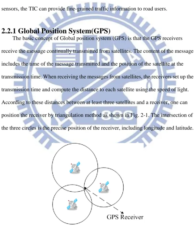
2.2.1 Global Position System(GPS)
The basic concept of Global position system (GPS) is that the GPS receivers receive the message continually transmitted from satellites. The content of the message includes the time of the message transmitted and the position of the satellite at the transmission time. When receiving the messages from satellites, the receivers set up the transmission time and compute the distance to each satellite using the speed of light. According to these distances between at least three satellites and a receiver, one can position the receiver by triangulation method as shown in Fig. 2-1. The intersection of the three circles is the precise position of the receiver, including longitude and latitude.
8
The computation of position is related to the time; so more precise the receiver’s clock is, more accurate position can be calculated. In addition, using the Doppler Effect on the transmission messages, one can also compute the instant speed of the receiver.
2.2.2 Gyroscope
A gyroscope is a device for measuring and maintaining orientation based on the principles of angular momentum. In present day, for supporting user interface and physical interactive software, many smartphones are installed with three-axis
gyroscope. It is capable of measuring the locations, the trajectory and acceleration of the six directions in the meantime. Compared with gravity sensors, which can only measure straight-line motion, the measurements by three-axis gyroscope are
three-dimensional orientation and position. With the features of the gyroscope, we can obtain the acceleration of the mobile devices on a traveling vehicle which is parallel to the direction of mobile devices moving on. The acceleration we obtained takes as the speed variation of the people carried the mobile device, and we detect whether the moving pattern has been changed suddenly.
2.2.3 Accelerometer
An accelerometer is a device that measure proper acceleration which is relative to free fall and felt by people and objects. Simply stated, the acceleration is a
measurement of how fast the speed of something itself is changed. Any point on the Earth’s surface is accelerating upwards relative to the local inertial frame, so an accelerometer at rest on the Earth’s surface will show approximately 1 g upwards. If we desire to obtain the acceleration of the objects without the effect of gravity, the “gravity offset” should be eliminated and corrected for the impact caused by Earth’s rotation relative to the inertial frame.
9
Same as many other scientific and engineering systems, accelerometers and gyroscopes usually are used together in the aspect of measuring an object’s moving behavior. For example, MEMS accelerometers are most regularly being used in the automotive airbag systems to detect the sudden deceleration caused by vehicle collision. In addition, we can use the accelerometer to conjecture the location while we are in tunnel where it not possible to receive the signals from satellites in GPS.
2.3 Broadcast Mechanism
In our thesis, we proposed a TIC, which would notify the probe cars by broadcast mechanism. Currently, we are able to broadcast messages in two ways: one is through roadside units of vehicular networks and the other is through cell broadcast cellular networks. In an intelligent transportation system, a roadside unit (RSU) is capable of communicating with the on-board units (OBU) of vehicles and connecting to the TIC [5]. A RSU serves an area where the TIC may collect the traffic information and the direction that a vehicle equipped with an OBU is moving. In addition, a RSU transmits the traffic information provided by the TIC on pre-determined channels. When an OBU enters a new communication zone, the OBU communicates with the new RSU by the previous channel information, the new RSU would inform the OBU the new channel information in order to continuously provide the traffic information from the TIC.
The other method is using cell broadcast of wireless networks [11]. The cell broadcast function is a specification in GSM network and also supported by Universal Mobile Telecommunication System (UMTS). Cell broadcast is designed for
simultaneously sending message to multiple users. Differed from short message service, point-to-point (SMS-PP), which is able to send messages to one or few users, the technique of cell broadcast is invented for broadcast same message to a particular area
10
with an assigned channel and the number of times. This cell broadcast function is suitable for broadcasting real-time traffic information to MSs.
2.4 The Properties of Traffic Jam
Traffic conditions are complicated and nonlinear, and they depend on the interaction of vehicles on road. Vehicles on the road network move as aggregative group and generate shock wave propagation. The movements of shock wave, such as forward and backward, rely on vehicle density in the area. When the density of the road network exceeds the maximal limitation, the traffic flow becomes unstable, and even a minor incident may cause traffic jams to make the vehicles into stop-and-go driving situation. The reasons of high traffic flow density are the bottlenecks of the road network and traffic flow gathered in certain area. A bottleneck of the road network is where the capacity is relatively lower than other sections of the road network. That is often a narrow part of a road network, such as roads with smaller number of lanes, a narrow bridge or tunnel, and locations where speed must be kept low for safety reasons. On the other hand, the locations where may gather traffic flow together are highway ramp, the intersection of highway and access road.
Treiber, er al reconstructed the spatiotemporal information of the road network from aggregated data of stationary traffic detectors, and they found that end locations of traffic jams may fixed at the bottleneck of the road networks [7]. With the increasing traffic flow and existence of a bottleneck, the start location of a traffic jam may travel upstream at a near-constant speed. In addition, we also found that when a vehicle gets into the traffic jam, the acceleration of vehicle is 3-4 times higher than that in
uniform-speed driving [8]. Depending on acceleration, driving speed and stop-to-go driving pattern, we can easily determine when and where a vehicle gets into or out
11
traffic jam.
2.5 VISSIM
Verkehr in Städten - Simulation (abbreviated as VISSIM), which means traffic in towns – simulation in English, is a microscopic traffic flow simulation [3]. In the real world, it is difficult to collect traffic data with a previous setup of collecting strategies and collected parameters of traffic condition, because it may make a great impact on economy and environment for complete traffic situation. With the emergence of VISSIM, we can efficiently collect and analyze traffic data from a variety of traffic conditions through this traffic flow simulator. VISSIM consists of two different components: traffic flow model and traffic control model. In the setup of traffic simulation, we determine the composition of traffic flow through traffic flow model. Separately, if there are traffic signals, we setup the details of traffic signals, such as the cycle of traffic lights, dwell time of tollgate, and public transit stop time, through traffic control model. Then, we can determine the traffic data that we would be interest at and the sample rate of the test bed and the simulator would generate the traffic data with the effect of these two models above for experimental analysis.
In this thesis, we established a variety of freeway traffic models such as, tollgate slowing down, ramp traffic merging onto highway, and changing the flow of traffic to cause a traffic jam. We also set up the sample rate of each vehicle to record its status. The status of a vehicle includes the coordinate (regarded as GPS coordinate), the speed, and the acceleration of the vehicle to assess the performance of the system we
12
Chpter 3 The System Design
3.1 System Overview
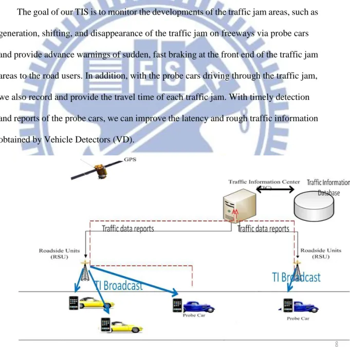
Our system uses a centralized architecture that consists of a traffic information center (TIC) and a group of probe cars. Fig. 3-1 depicts the system architecture. The functions of each component will be described below.
The goal of our TIS is to monitor the developments of the traffic jam areas, such as generation, shifting, and disappearance of the traffic jam on freeways via probe cars and provide advance warnings of sudden, fast braking at the front end of the traffic jam areas to the road users. In addition, with the probe cars driving through the traffic jam, we also record and provide the travel time of each traffic jam. With timely detection and reports of the probe cars, we can improve the latency and rough traffic information obtained by Vehicle Detectors (VD).
13
The traffic information center (TIC) is a centralized server which not only receives the reports from probe cars, but also provides timely traffic information to road users including the probe cars and the general via the broadcast function of Roadside Units (RSU) of vehicular communication networks or the base-stations of the public wireless networks. The TIC has a global view of the entire road network, that is, the TIC maintains the status of each traffic jam detected by probe cars. The status information include the start position, end position and travel time of each traffic jam and the information can be broadcasted to probe cars for advance awareness of the traffic condition of the road they may travel. Since the traffic information is updated by the TIC based on the reports from the probe cars, the TIC would immediately broadcast the updated information to the road users. Simply stated, the TIC broadcasts are triggered by the reports from the probe cars. On the other hand, the probe cars would report to the TIC when they detect the status of a traffic jam has changed to a certain degree.
We assume that each probe car is equipped with a smartphone which is capable of GPS positioning, acceleration measurement, and wireless data communication. With the increasing advance of sensing abilities on smartphones, such as positioning and acceleration, the driving behavior of a vehicle can be constantly monitored by the on-board smartphones carried by the driver or passengers. Obtaining the traffic
information broadcasted from the TIC via RSUs or BSs, a smartphone is able to detect the difference between the traveling behavior of itself and the broadcasted traffic information. If the probe car detects the significant shift of the boundaries (front-end or rear-end) of a traffic jam, the creation of a new traffic jam, or the disappearance of a traffic jam, the probe car would transmit the changes of the traffic jam to the TIC. While the TIC receives the updates from probe cars, it would broadcast the latest traffic
14
information to the road users.
3.2 Traffic Information Center
The TIC receives reports from the probe cars, maintains the status of each traffic jam detected, and broadcasts the status. To reduce the number of reports, the TIC also specifies reporting thresholds. When the difference between the broadcasted status and the travel data experienced by a probe care is larger than the thresholds, the probe car reports the change of status to the TIC. After receiving the report, the TIC modifies the status of the reported traffic jam accordingly. Table 3-1 lists the notation and definition of the status variables used to describe the details of traffic jam events. Lstart denotes the
start location of a traffic jam on the road network detected by probes, and TS denotes the
time when the probes detect themselves getting into a traffic jam. Lend denotes the end
location of a traffic jam on the road network, and TE denotes the time when the probes
detect themselves getting out of a traffic jam. In addition, TT denotes the travel time which the probes travel during the whole traffic jam. The TIC maintains an list of traffic jams, and the status variables of each traffic jam including the start position of the traffic jam, the report time of the start position, the end position of the traffic jam, the report time of the end position, and the travel time needed to pass the traffic jam. The TIC broadcast the status of a traffic jam only to the vehicles on the related road segment, i.e., only to the vehicles heading to or traveling in the traffic jam. This can be done by
Table 3-1 Parameters used in the TIC.
Notation Definition Value
Lstart The start position of the traffic jam --
TS The report time of the start position --
Lend The end position of the traffic jam --
TE The report time of the end position --
15
broadcast the information on a specific channel of the RSUs on the related road segment or by the cell broadcast function of the public wireless networks.
3.3 Probe Cars
The report policy of probe cars is the core of our solution. When we drive into a traffic jam on a highway, we may first brake fast and then drive in a stop-and-go fashion. According to the experience, a probe car observes its acceleration and speed at the same time to determine the boundaries of a traffic jam. Note that not all traffic jams cause fast braking, the stop-and-go moving pattern alone can also determine the beginning of a traffic jam.
Table 3-2 lists the notation and definition of variables used in our probe car report policy. The measurement rate of the GPS receiver and acceleration sensors is once per second, i.e., we can get the speed, location information and acceleration of the vehicle
Table 3-2 Parameters used in the probe car report policy.
Notation Definition Value
StatusPC The status of the vehicle 0 = in free flow
1 = in traffic jam
LPC The current location of the probe car obtained
from GPS
--
VPC The current speed of the probe car --
APC The current acceleration of the probe car
paralleled to the heading direction
--
W The buffer size Constant
VSMS The space mean speed of the of the probe car --
Vin The speed threshold to determine the existence
of a traffic jam
--
Ain The acceleration threshold to determine the
existence of a traffic jam
Ain < 0
Vout The speed threshold to determine probe car out
of traffic
Vout > Vin
Dmod The distance threshold to to modify the start and
end positions of a traffic jam
--
Dgen The distance threshold to determine to generate
a new traffic jam or eliminate a traffic jam
16
each second. In addition, a probe car records the measurements with timestamps. Measurements are stored in a buffer of size W and are used to compute the space mean speed. Let Locationn denote the current location, and Locationn-W denote the location of
the probe car W seconds before. The space mean speed can be obtained as follows,
(3.1)
While the probe car first appears in the road network, it would receive the traffic information from the TIC. According the traffic information, the probe car determines whether it is in a traffic jam or not by its location and initializes its status StatusPC, If
the probe car is in a traffic jam, StatusPC would be 1; otherwise, StatusPC would be 0.
A probe car determines that it drives into a traffic jam based on the following two conditions:
(1) VPS < Vin and APS < Ain
(2) VSMS < Vin
Condition 1 checks if the probe car brakes fast and its speed drop below Vin, a
speed threshold of a traffic jam. Condition 2 checks if the space mean speed in the last
W seconds is blow Vin.
Fig. 3-2 depicts the flow chart of a probe car after it get the measurements of its location, speed and acceleration. If the probe car is not in a traffic jam, i.e., StatusPC
equals to 0, it first checks if condition 1 is met. If so, the probe car has just entered a traffic jam with fast braking applied, and the start position of the traffic jam measured by the probe car is LPC. The probe car would record the current time, discard all traffic
17 GPS Information LPC VPC APC StatusPC == 1 Add GPS information to the buffer VPC < Vin APC < Ain Add GPS information to the buffer
(1)Clean the data in the buffer (2)Add the GPS information to the buffer
(3)Statusps = 1 VSMS < Vin Do nothing StatusPC = 1 VSMS > Vout Do nothing StatusPC = 0 No No No No Yes Yes Yes Yes
Fig. 3-2 A Flow chart of a probe car detecting traffic jams
data in the buffer and add the current one in the window. The probe car would also check if it is a new traffic jam or it is an old traffic jam, which has shifted its start location. According to the report policy, which will be discussed later, the probe car may report the change to the TIC. If condition 1 is not met, the probe car checks it condition 2 is met. If so, the probe car has entered a traffic jam W seconds ago without applying fast braking. The start position of the traffic jam is the first record stored in the buffer. The probe car sets StatusPC to 1, and performs the report policy to determine if it
needs to send a report to the TIC.
On the other hand, if StatusPC equals to 1, the probe car checks if VSMS is larger
than Vout, a space mean speed threshold, which determines whether a probe car has it
18
seconds. If the condition is met, the time when the probe drove out of the traffic jam is
W seconds ago, and the end position of the traffic jam is also stored in the record W
seconds ago. With the recorded time of getting into the traffic jam, the probe car can easily compute the travel time of the current traffic jam. In order to confirm a probe car getting into and out of a stop-and-go traffic condition, we formulate the condition of getting into a traffic jam is stricter than that of getting out of a traffic jam. Simply stated, the Vin is smaller than Vout.
After a probe car detects the start location or the end location of a traffic jam, the probe car compares the detected information with that broadcasted from the TIC to determine if it needs to inform the TIC to modify the traffic information. When the start location of a traffic jam is detected by a probe car, let LMS denote the start location
detected by the probe, and Lstart denote the start positon of the nearest traffic jam
broadcasted by the TIC. The probe car compares LMS and Lstart, and two distance
thresholds are used to determine if the probe car needs to send a report and the type of report to be sent. First, if the distance between LMS and Lstart is less than Dmod, a
modification threshold, the probe does not report the change to the TIC. The reason is because GPS location measurements are of unavoidable errors and minor changes of the start location do not need to be reported. Second, if the distance between LMS and
Lstart is larger than Dmod, bust less than Dgen, the probe car informs the TIC that the start
location of the traffic jam have shifted to LMS. Last, if the distance between LMS and Lstart
is larger than Dgen, the probe car sends a report of a new detected traffic jam to the TIC.
When a probe car detects the end position of a traffic jam and computes the travel time of the traffic jam, if the traffic jam is a new one detected by the probe car, the probe car reports the end location and travel time of the traffic jam to the TIC. Otherwise, if the
19
distance between LMS and Lend is larger than Dmod, the probe car reports to the TIC that the end position has changed.
In addition, if a probe is in a smooth traffic and passes the start location LMS of the
traffic jam over Dgen, it means the probes pass the traffic jam for a certain distance and
don’t detect the traffic jam. It notifies the TIC to remove the traffic jam. If a probe is in a traffic jam and passes the start location LMS of the next traffic jam, that means there
are some traffic jams need to merge. It notifies the TIC to merge the traffic jams. Furthermore, if the difference between the travel time in passing through the traffic jam measured by the probe car and that broadcast by the TIC is more than 5%, the probe car informs the TIC of the measured travel time.
20
Chpter 4 Evaluation and Analysis
4.1 Simulation Environment and Parameters
To evaluate the performance of our system, we simulate three traffic scenarios on highway: a single-lane freeway with an interchange, a three-lane freeway with an interchange and a single-lane freeway with a tollgate. We have developed a simulation system that uses VISSIM, a microscope traffic model simulator, to produce traffic jams. Based on the traffic jam movement on the simulated road, we can estimate the
performance of the system we proposed. For each vehicle on the simulated road, we set up VISSIM to record the status of each vehicle once a second. The recorded status of a vehicle includes the vehicle number, the vehicle type, the vehicle speed, the vehicle acceleration, and the vehicle location. Random samples of the vehicles are our probes, i.e., the vehicles carry smartphones as probes. In addition, since the location
measurements from GPS receivers cannot be 100% accurate, we also inject random errors in the probe location to study the effects of GPS locations errors.
In order to evaluate the performance of the system, we observe several
performance parameters. First, we observe the communication cost of our system. The communication cost includes the number of broadcast messages from the TIC. The broadcast messages can be further classified into the start position messages, the end position messages, the travel time messages and traffic jam removal messages. Second, we compute the location errors between the broadcasted start/end locations and the locations measured by the vehicles. Third, we compute the time differences between the broadcasted travel time and the actual travel time experienced by the general vehicles and the probes. Last, we compute the Advance Warning Coverage (AWC)
21
which is the percentage of general vehicles that receive advance warning, i.e., the existence of a traffic jam, before encountering the traffic jam. In addition, we study the effects of probe penetration rate on the performance parameters described above. Table 4-1 lists the threshold values used in our experiments. According to the speeds of the vehicles passing through the simulated road, we define that the speed of vehicles between 40 km/h and 70 km/h represents the vehicles are in a traffic jam. Therefore, we set VIN is 40 km/h and VOUT is 70 km/h. We observe the acceleration of vehicles in a smooth traffic and getting into traffic jam, and chose AIN to be -1.5 m/s2. In order to reduce the number of reports from the probe cars and maintain the timely traffic information with small location errors, we determine that Dmod is 100 m and Dgen is 200 m.
Table 4-1 The threshold values used in the simulation model
Parameter Value VIN 40 km/h AIN -1.5 m/s2 VOUT 70 km/h Dmod 100 m Dgen 200 m
4.2 Performance Evaluation
4.2.1 A Single-Lane Freeway with an Interchange Model
22
In order to reduce the complexity of the traffic condition, first, we study a single-lane freeway with an interchange, as shown in Fig 4.1. We simulate a 9-km single-lane freeway with an interchange at 4 km post. There is a 200-m long
acceleration lane at the intersection of the freeway and the interchange. The speed limit on the freeway is 90 km/h, and the desired speed of each vehicle is uniformly
distributed between 85 km/h and 120 km/h. The traffic flow on the freeway before the interchange is 1000 vehicle/hour. By controlling the traffic flow input from the
interchange, we can create traffic jams on the freeway. Table 4-2 lists the traffic flow input from the interchange as the simulation goes on. Initially, there is no traffic input from the interchange. At simulation time 900 sec, we generate a heavy traffic flow input (1000 veh./h) from the interchange to cause a traffic jam on the freeway, and gradually decrease the traffic flow input from the interchange to remove the traffic jam. The total simulation time is 1 hour, and the status of simulated vehicles recorded by VISSIM is input to a simulation program which performs the functions of both the TIC and the probes.
Table 4-2 The traffic flow input from the interchange
Simulation Time (second) Traffic Flow (veh./h)
0~900 0
900~1800 1000
1800~2400 700
2400~3000 300
Based on the status of simulated vehicles, we depict the ground truth, the traffic conditions with respect to the simulation time and the freeway location in Fig 4.2. The X-axis is the simulation time and the Y-axis is the highway location starting from 0 km post. The green areas represent that the speed of the vehicles is higher than 70 km/h (VOUT), the yellow areas represent that the speed of the vehicles is between 40 km/h
23
Fig 4.2 The ground truth and the detected start and end positions of traffic jams
under 40 km/h (VIN). In other words, in the green areas, the traffic is a free flow, and in
the red areas, the traffic is congested. We can observe that when a heavy traffic flow starts to input from the interchange at simulation time 900 sec., the interchange becomes the bottleneck of the freeway, and a traffic jam builds up before the interchange. The start position of the traffic jam travels upstream, while the end (a)
24
position remains almost fixed. While the traffic flow input to the interchange decreases gracefully, the traffic jam reduces its area, separates to small traffic jams and
disappears.
Fig. 4.2(b) depicts the start and end positions of traffic jams detected by the vehicles in the road network. Each blue dot represents a start position detected by VIN
and AIN, and each black dot represents a start position detected by the space mean speed
being lower than VIN. Each purple dot represented a detected end position. From the
ground truth of the simulated road, we found that the traffic jams in the road network can be bounded by the start and end position detected by the probes. The proportion of the start positions that is detected by the space mean speed alone is much less (less than 5%) than that detected by the instantaneous speed and acceleration.
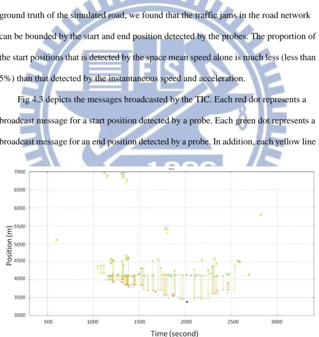
Fig 4.3 depicts the messages broadcasted by the TIC. Each red dot represents a broadcast message for a start position detected by a probe. Each green dot represents a broadcast message for an end position detected by a probe. In addition, each yellow line
25
represents a broadcast message for the start position, end position and travel time of a traffic jam. The figure shows that the report policy roughly depicts the traffic jam in the road network. While the traffic jam is starting disappearance, the number of broadcasts increases.
Table 4-3 lists the performance metrics of the system we proposed and the effects of GPS position errors. In the column of start position reports, the number to the right of the slash is the total number of start positions of the traffic jams detected by the probes. The number to left of the slash is the number of the start position reports sent by the probes, after the probes detect that the difference between the detected start position and the start position broadcasted by the TIC exceeds the distance threshold. Equally, in the column of end position reports, the number to the right of the slash is the total number of end positions detected by the probes. The number to the left of the slash is the number of the end position reports sent by the probes, after the probes detect that the difference of the end position or the difference of the travel time exceeds the
corresponding threshold. When the GPS positioning is assumed to be no error, there are 100 broadcast messages from the TIC, i.e., 100 reports sent from the TIC. The 100 reports include 33 start position reports, 44 end position reports and 23 segment
Table 4-3 The effects of GPS position errors
GPS positioning errors The no. of broadcasts Start position reports/ Start positions detected End position reports/ End positions detected Segment removal reports Location error Travel Time error AWC No error 100 33/72 44/100 23 79.8 10.4% 90.7% 20m 103 34/74 45/102 24 101.09 12.3% 89.5% 50m 187 58/126 84/155 45 93.1 11.8% 89.2%
26
removal reports. The results indicate that these report thresholds reduce over 50% of the start position and end position reports sent by the probes, while providing a high AWC of 90%, a low location of less than 80 m, and a small travel time error of 10.4%. In addition, when GPS positioning errors is 20 m in average, the number of broadcast messages increases by 3, the average location error increases by 20 m, the travel time error increases by 2%, and the AWC decreases by 1%. When the GPS positioning errors are 50 m, the number of broadcast messages increases by about 90%, while other performance metrics remain about the same as those when GPS positioning errors are 20 m.
We also observe the impact of different penetration rates of the probes. Fig 4.4 depicts the impact of the probe penetration rate. With the increase of the penetration rate, the number of broadcasts increases almost linearly. However, as the penetration rate increases, the location and time errors decrease only slightly.
27
4.2.2 Multi-Lane Freeway with an Interchange Model
Fig 4.5 A multi-lane freeway with an interchange
For the realistic traffic model, we study a multi-lane freeway with an interchange, as shown in Fig 4.5. We simulate a 9-km, 3-lane freeway with a single-lane interchange at 4 km post. There is a 200-m long acceleration lane at the intersection of the freeway and interchange. The speed limit on the freeway is 90 km/h, and the desired speed of each vehicle is uniformly distributed between 85 km/h and 120 km/h. The traffic flow on the freeway before the interchange is 3000 vehicle/hour. By controlling the traffic flow input from the interchange, we can create traffic jams on the freeway. Table 4-4 lists the traffic flow input from the interchange as the simulation goes on. Initially, there is no traffic input from the interchange. At simulation time 900 sec., we generate a heavy traffic flow input (3000 veh./h ) from the interchange to cause a traffic jam on the freeway, and gradually decrease the traffic flow input from the interchange to remove the traffic jam. The total simulation time is 1 hour, and the status of simulated vehicles recorded by VISSIM is input to a simulation program which performs the functions of both the TIC and the probes.
Table 4-4 The variation of traffic flow from interchange
Simulation Time(second) Traffic Flow(veh/h)
0~900 0
900~1800 3000
1800~2400 2000
2400~3000 1000
Based on the status of simulation vehicles, we depict the ground truth and the traffic conditions with respect to the simulation time and the freeway location in
28
Fig 4.6. The X-axis is the simulation time and the Y-axis is the highway location starting from 2 km post to 6 km post. In the green areas, the traffic is a free flow, and in the red areas, the traffic is congested. We can observe that when a heavy traffic flow starts to input from the interchange at simulation time 900 sec., the interchange becomes the bottleneck of the freeway, and a traffic jam builds up before the
Fig 4.6 The ground truth and the detected start and end positions of traffic jams
(b) (a)
29
interchange. While the traffic flow input to the interchange decreases gracefully, the traffic jam reduces its area, separates to small traffic jams and disappears. Unlike the single-lane freeway with an interchange model, vehicles are able to change lane while the front vehicles slow down. So, in this simulation model, besides the bottleneck of the road network, there are few traffic jams in the road network. Fig. 4.6(b) depicts the start and end position of traffic jams detected by the vehicles in the road network. From the ground truth of the simulated road, we found that the traffic jams in the road network can be bounded by the start and end position detected by the probes. The start position of the traffic jam travel upstream, while the end position remain almost fixed at the km post of the interchange.
Fig. 4.3 depicts the message broadcasted by the TIC. It shows that the report policy roughly depicts the traffic jams in the road network. During the period of traffic jams starting generation and disappearance, the number of broadcasts increases. In addition, the setup of distance and time thresholds efficiently reduce the number of
30
broadcasts.
Table 4-5 lists the performance metrics of the system we proposed and the effects of GPS position errors. When the GPS positioning is assumed to be no error, there are 72 broadcast messages from the TIC, i.e., 72 reports sent from the TIC. The 72 reports include 27 start position reports, 30 end position reports and 23 segment removal reports. The results indicate that these report thresholds reduce over 80% of the start position and end position reports sent by the probes, while providing a high AWC of 96%, a low location of less than 55m, and a small travel time error of 12.3%. In addition, when GPS positioning errors is 20 m in average, the number of broadcast messages increases by about 95%, the average location error increases by about 4 m, the travel time error decreases by about 2.5%, and the AWC decreases by 0.5%. When the GPS positioning errors are 50 m, the number of broadcast messages increases by about 90%, the average location error increases by about 25 m, the travel time error increases by about 2.5%, and the AWC decreases by 1.5%. Compared with single-lane model, the AWC is higher. The report thresholds reduce the probe cars reports more efficiently than that for the single-lane model. In addition, the location errors of start position of
Table 4-5 The effects of GPS position errors
GPS positioning errors The no. of broadcasts Start position reports/ Start positions detected End position reports/ End positions detected Segment removal reports Location error Travel Time error AWC No error 72 27/147 30/201 15 51.3 12.3% 96.6% 20m 151 48/169 81/222 22 55.27 9.8% 95.9% 50m 392 120/469 195/522 77 79.8 12.2% 94.5%
31
traffic jams are a little slighter than that of single-lane model. The reason caused the above three feature is highly related to the difference of the simulation models which bring about the distribution of the traffic jam.
We also observe the impact of different penetration rates of the probe cars. Fig 4.8 shows the impact of the probe penetration rate. As the penetration rate increases, the number of broadcasts increases at a lower rate than that in single-lane freeway model. In addition, Location error is lower than that of the single-lane model.
Fig 4.8 The effects of the penetration rate of probe cars
4.2.3 Single-Lane Freeway with a Tollgate Model
For another commonly seen situation in the freeway causing the traffic jam, tollgate, we also study a single-lane freeway with a tollgate model. We simulate a 6-km single-lane freeway with a tollgate at 4 km post. The speed limit on the freeway is 90 km/h, and the desired speed of each vehicle is uniformly distributed between 85 km/h and 120 km/h. In addition, the dwell time at the tollgate is 3 seconds, and the dwell time of each vehicle is uniformly distributed between 2 sec. and 4 sec.. By controlling the traffic flow input from the freeway, we can create traffic jams before the tollgate. Table
32
4-6 lists the traffic flow input from the freeway as the simulation goes on. Initially, we generate a heavy traffic flow input (1000 veh./h), and gradually decrease the traffic flow input from the freeway to cause the movement of the start positions of traffic jam. The total simulation time is 1 hours, and the status of simulated vehicles recorded by VISSIM is input to a simulation program which performs the functions of both the TIC and the probes.
Table 4-6 The traffic flow input from the interchange
Simulation Time(second) Traffic Flow(veh/hr)
0~600 1000
600~1200 500
1200~2000 300
2000~3600 100
Based on the status of simulation vehicles, we depict the ground truth, and the traffic conditions with respect to the simulation time and the freeway location in Fig 4.9. The X-axis is the simulation time and the Y-axis is the highway location starting from 2 km post to 5 km post. We can observe that when a heavy traffic flow starts to input from the freeway at the beginning, the tollgate becomes the bottleneck of the freeway, and the start position of the traffic jam travels upstream. However, the end position remains almost fixed at the tollgate. While the traffic flow input to the tollgate decreases. The traffic jam reduces its area, but not disappears due to the persistent existence of bottleneck on the freeway.
Fig 4.9(b) depicts the start and end position of traffic jams detected by the vehicles in the road network. From the ground truth of the simulated road, we found that the traffic jams in the road network can be bounded by the start and end position detected by the probes. Furthermore, while the distance of traffic jam decreases, the number of
33
Fig 4.9 The ground truth and the detected start and end positions of traffic jam
the start positions detected by vehicle also decreases. Fig 4.10 depicts the message broadcasted by the TIC. At the beginning, while the traffic flow is increasing, the start positions of the traffic jam travel upstream rapidly and the number of broadcasts is higher. After the traffic flow decreasing, the number of broadcasts decreases relatively.
Table 4-7 lists the performance metrics of the system we proposed and the effects of GPS position errors. When the GPS positioning is assumed to be no error, there are (b)
34
Fig 4.10 the message the system broadcasted
17 broadcast messages from the TIC, i.e., 17 reports sent from the TIC. The 17 reports include 7 start position reports, 10 end position reports and 0 segment removal reports. Because of the tollgate permanently existing on the road network, there is no traffic jam removal in this simulation model. The results indicate that these report thresholds reduce over 75% of the start position and end position reports sent by the probes, while providing a high AWC of 97.3%, a low location of less than 70 m, and a small travel
Table 4-7 The effects of GPS position errors
GPS positioning errors The no. of broadcasts Start position reports/ Start positions detected End position reports/ End positions detected Segment removal reports Location error Travel Time error AWC No error 17 7/30 10/31 0 67.3 9.1% 97.3% 20m 34 11/33 23/31 0 73.1 10.5% 96.9% 50m 38 12/51 26/35 0 87.4 15.1% 96.1%
35
time error of 9.1%. In addition, when GPS positioning errors is 20 m in average, the number of broadcast messages increases by 100%, the average location error increases by 5 m, the travel time error increases by 1.4%, and the AWC decreases by 0.4%. When the GPS positioning errors are 50 m, the number of broadcast messages increases by 4, the average location error increases by about 14 m, the travel time error increases by about 5%, and the AWC decreases by 0.8%. Compared with the above two simulation models, the communication costs are lower because of relatively stable traffic
conditions. As GPS position errors increase, the communication costs increase minor. We also observe the impact of different penetration rates of the probes. Fig 4.11 shows the impact of the probe penetration rate. As the penetration rate increases, the number of broadcasts increases at a lower rate. In addition, the AWC is the highest in the three traffic simulation models.
36
Chpter 5 Conclusions
In this thesis, we present a FCD-based traffic information system that can monitor the traffic jam areas on freeway and their travel times. The system consists of a central traffic information center (TIC) and a group of smartphones embedded with GPS receiver and accelerometer, functioning as probes. The probes receive the current status of traffic jams broadcasted by the TIC, and compare the status with the traveling data measured by their sensors. If the start location, end location or travel time of a traffic jam has changed by pre-determined thresholds, the probes report the change to the TIC. After receiving reports from the probes, the TIC would broadcast the updated
information of the traffic jam to the probes and general road users.
We have performed computer simulation using VISSIM to evaluate the
performance of our system. The simulation results indicate that our system can reflect the dynamic change of traffic jams and provide road users the timely information of the traffic jams. The absolute errors of the start position and end position of a broadcasted traffic jam are less than 100 m, and the absolute error of the travel time of a broadcasted traffic jam is less than 10%. In addition, over 90% of general vehicles receive traffic jam information, before they encounter a traffic jam, i.e., they receive advance warning and precautions can be taken by the drivers to avoid sudden fast braking, which may cause traffic accidents. However, there are still some problems that need to be solved. First, as the penetration rate of probes in the road network increases, the number of reports would increase linearly. Further research is therefore necessary to to reduce the number of reports and the number of broadcasts when the number of probes increases. Second, the simulation models that we constructed only generate small-scale traffic
37
jams and we assume that the traffic jams appear in the same service area of a RSU. When a traffic jam spans over the service areas of several RSUs, the broadcast
mechanism needs to be modified for estimating the travel time and localizing a traffic jam.
The system proposed in this thesis is based on a centralized architecture, which puts most of the computation load to the probes and only detects two traffic states on highway (i.e. smooth traffic and traffic jam). With the increasing computation power of handheld devices and powerful sensing ability, it is possible for the probes to detect more elaborated traffic conditions. In the future, we plan to improve our system to detect more detailed traffic information, such as traffic situations on different lanes of a highway.
38
Reference
[1] J. C. Herrera, et al., “Evaluation of traffic data obtained via GPS-enabled mobile phones: The Mobile Century field experiment,” Transportation Research Part C, No. 18, pp. 568-583, 2010.
[2] Lane, N, Miluzzo, E, Lu, H., Peebles, D., Choudhury, T., Campbell, A. (2009), A Survey of Mobile Phone Sensing. Ad Hoc and Sensor Networks. IEEE Comm. Sept 2010.
[3] Y.B Youngbin Yim and Randall Cayford, “Investigation of vehicles as Probes Using Global Positioning System and Cellular Phone Tracking: Field Operational Test”, Report UCB-ITS-PWP-2001-9. California PATH Program, Institute of Transportation Studies, University of California, Berkeley, CA, 2001
[4] M. Fellendorf, 1994, VISSIM: A microscopic simulation tool to evaluate actuated signal control including bus priority, Technical paper, Session 32, 64th ITE Annual Meeting, Dallas.
[5] Lars Wischhof, Andre Ebner, Hermann Rohling, Matthias Lott, and Rüdiger Halfmann, “SOTIS - A Self-Organizing Traffic Information System”, in Proceedings of the 57th IEEE Vehicular Technology Conference, 2003.
[6] Byoung Heon Lee, Gwangmycoog-si(KR), “ System and Method for Providing Channel Information of Roadside Unit”, 2003, US 6,829,531 B2
[7] C. Perkins, Ad Hoc Networking, Addison-Wesley, 2000.
[8] M. Treiber, D. Helbing, .Realistische Mikrosimulation von Strassenverkehr mit einem einfachen Modell., 16th Symposium Simulationstechnik ASIM 2002, Rostock, September 2002.
39
(Transportation Research Board, National Research Council, Washington, D.C., 1975).
[10] B. Kerner, C. Demir, R. Herrtwich, S. Klenov, H. Rehborn,M. Aleksic, and A. Haug, “Traffic State Detection with Floating Car Data in Road Networks”, in IEEE Proc. on Intelligent Transportation Systems, 2005.
[11] Darrel J. Van Buer, Son K. Dao, Xiaowen Dai, et al., “Traffic Notification System for Reporting Traffic Anomalies Based on Historical Probe Vehicle Data”, US 7460948, 2008.
[12] J. P. Castro, “The UMTS Network and Radio Access Technology”, John Wiley & Sons, 2001.