增量選取在平行化線性亂數產生器的應用

國

立

交

通

大

學

統計學研究所

碩

士

論

文

增量選取在平行化線性亂數產生器的應用

Parallel Linear Random Number Generators

With Different Increment Shifts

研 究 生：謝國偉

指導教授：盧鴻興 教授

增量選取在平行化線性亂數產生器的應用

Parallel Linear Random Number Generators

With Different Increment Shifts

研 究 生：謝國偉 Student：Kuo-wei Hsieh

指導教授：盧鴻興 Advisor：Henry Horng-Shing Lu

國 立 交 通 大 學

統計學研究所

碩 士 論 文

Submitted to Institute of Statistics College of Science

National Chiao Tung University in Partial Fulfillment of the Requirements

for the Degree of Master

in Statistics June 2006

Hsinchu, Taiwan, Republic of China

感謝

七百多天的日子不算長，卻足以讓夠讓我回味無窮。感

謝指導老師盧鴻興教授與美國孟斐斯大學數學科學系老師

鄧利源教授耐心地傾囊相授，與您們的面談與魚雁往返，激

勵我不少靈感與專業知識的增長；謝謝交通大學統計所的師

長、同學及學弟妹，豐富了我的學識與碩士生活；最後特別

感謝最後半年，在美國芝加哥大學認識的實驗室朋友，以及

在內湖的一位摯友，你們的友情與鼓勵，為我劃下碩士生涯

完美的句點！

摘要

線性同餘法（

linear congruential generator，LCG）

與 k 階乘

餘法（

multiple recursive generator，MRG

）至今仍為亂數產生器

常使用的兩大線性方法；而近日，由於電腦處理器成本下

降，平行化計算因而被廣泛研究與使用，以改善因分析與模

擬資料量與日俱增，電腦運算效率降低之問題。除此之外，

平行化處理亦可能增強許多模擬數據時所需具備的統計性

質，如隨機性等。傳統平行化線性亂數產生器之方式，譬如

使用不同初始值，多僅改善運算速度，對於統計性質的改

變 ， 則 助 益 不 大 ； 但 藉 由 改 變 線 性 亂 數 產 生 器 的 增 量

（increment），則可坐收同時改善速度與性質之效，且計算

簡單，易於推廣，尤其輔以平行設計之跳蛙法（leapfrogging

method）

，綜效較順序切割法（sequence splitting method）更

Abstract

Two major linear random number generators (RNGs), the linear

congruential generator (LCG) and the multiple recursive generator

(MRG), have been widely studied and used for many decades. Nowadays,

as the price decreasing of computer processors, parallelization of the

generators is being concerned for, at least, the computational efficiency

purpose. Besides, the proper design of parallel generator may also

improve some statistical properties such as randomness. The Parallel

linear random number generator with different increment shifts is

efficient and feasible because the change of the increments only shifts the

hyperplanes of the linear RNG. Additionally, parallelizing through the

leapfrogging method can further improve than through the sequence

splitting method.

Table of Contents

Chapter 1. INTRODUCTION 1 Chapter 2. SERIAL LINEAR RANDOM NUMBER GENERATORS 2 2.1 Linear Congruential Generator (LCG) 2 2.2 Multiple Recursive Generator (MRG) 3 2.3 DX-k-s Random Number Generators 4 Chapter 3. STATISTICAL TESTS AND CRITERIA 5 3.1 Uniformity 5 3.2 Randomness 6 3.3 LATTICE STRUCTURE 7 Chapter 4. PARALLEL LINEAR RANDOM NUMBER GENERATORS 8 4.1 Sequence Splitting 9 4.2 Leapfrogging 9 Chapter 5. PARALLELIZATION WITH DIFFERENT INCREMENT SHIFTS 9 5.1 Minkowski Bases of the LCG 9 5.2 Parallel Design of Increment Shifts 12 5.3 Serial Correlation 13 5.4 Lattice Structures 16 5.5 Inter-processor Correlation 17 5.6 Absorbing States 19 Chapter 6. SIMULATION RESULT 25 Chapter 7. CONCLUSION AND DISCUSSION 26

REFERENCE 28 APPENDIX 31

1. INTRODUCTION

It is very important to develop a random number generator (RNG) to generate pseudo-random numbers for simulations in computers (Knuth 1998). With the developed of parallel computing in modern computer technology, this study is aiming at the design of parallel linear random number generators with different increment shifts for simulations with parallel computing.

The linear congruential generator (LCG) has been widely used for its simplicity and theoretical properties since the first proposal in Lehmer (1951). With the increasing demand of high quality random numbers, the multiple recursive generator (MRG) and other methods were developed afterwards (L’Ecuyer, Blouin and Couture, 1993, Knuth 1998, Deng and Xu, 2003). The MRG greatly extends the period of the random sequence and improves properties of the LCG. It is challenging to determine the parameters in the MRG that improve the properties of a RNG. The DX generator has been proposed by Deng and Xu (2003) to select parameters in the MRG that prolongs the period of random sequences and improves the efficiency of simulation. As the price decreasing of computer processors nowadays, it becomes very economic and efficient to generate numbers through parallelization by many computers. With a proper design of algorithms, it becomes feasible to shorten the computational speed and strengthen randomness of the output (Gentle, J. E. 2003). This study will propose methods to parallelize a linear generator by using different increment values. The theoretical and empirical properties will be explored in this study.

2. SERIAL LINEAR RANDOM NUMBER GENERATORS

2.1 Linear Congruential Generator (LCG)

The method of LCG has been proposed by Lehmer (1951). This recursive generator has the following form:

Xi = (aXi – 1 + c) mod m, (2.1) Ui = Xi / m, (2.2)

where a, c, m, and X0 are integers; m > 0 is the modulus parameter; 0 < a < m is the

multiplier parameter; 0 ≤ c < m is the increment parameter; X0 is the starting value or

the seed, 0 ≤ X0 < m when c ≠ 0 and 0 < X0 < m otherwise.

The performances of linear congruential generators differ drastically considering the changes of a, c, and m. These parameters hence ought to be chosen very cautiously so that the resulting pseudorandom numbers possesses good properties, such as long period, uniformity, randomness, and so forth. Since the random number of Xi is obtained from the remainder after the modulo operation of m, the possible

outcome Xi is in the set of S = {0, 1, 2, …, m – 1}. An LCG is said to attain the full

period m if and only if the following theorem is satisfied (Knuth 1998): (1) c is relatively prime to m;

(2) q is a factor of (a – 1), if q is a prime factor of m; (3) (a – 1) is a multiple of 4, if m is also a multiple of 4.

The LCGs can be classified into two types, mixed (c > 0) and multiplicative (c = 0). Apparently, the full period does not exist in the multiplicative case because c = 0 is a multiplier of any integer m. Also, 0 is an absorbing state in this case. Instead, its maximum period, m – 1, is obtained when a is a primitive element modulo m. Furthermore, it is widely used in 32 bit computers with the multiplicative LCGs, m = 231 – 1 and a = 7k where k is a primitive root such as a = 75 = 16,807.

2.2 Multiple Recursive Generator (MRG)

The multiplicative LCG can be extended to the higher order recursively by adding up the previous k pseudorandom numbers. This is called as the multiple recursive generator (MRG), which is defined as follows:

Xi = (a1Xi – 1 + a2Xi – 2 +…+ akXi – k) mod m, (2.3) Ui = Xi / m, (2.4)

where k is the order. The absolute values of the multipliers a1, a2, …, ak and the

starting values X0, X1, …, Xk – 1 may be any numbers except for all zeros. In addition, ak should be nonzero. If k = 1, the MRG degenerates to the multiplicative LCG.

The maximum period of an MRG is improved to mk – 1 on condition that f(x) =

xk – a1xk – 1 –…– ak – 1x – ak is a primitive polynomial modulo m. Alanen and Knuth

(1964) and Knuth (1998) showed the following criteria to find a1, a2, …, ak:

(1) (–1)k – 1ak must be a primitive root modulo p;

(2) the polynomial xr must be congruent to (–1)k – 1ak, modulo f(x) and m;

(3) the degree of xr/q mod f(x), using polynomial arithmetic modulo m, must be positive, for each prime factor q of r.

where r = (mk – 1)/(m – 1).

The MRG has improved the statistical properties for an RNG with slight increase of computational time because this generator requires more multiplication and calculation. Also, the criteria for selecting multiplier parameters requires the prime factorization of r = (pk – 1)/(p – 1), which is challenging in seaching when p and k are larger (Knuth 1998).

L’Ecuyer, Blouin, and Couture (1993) made an attempt to find some MRGs for k ≤ 7. With m = 231 _{– 1, they suggested a sixth-order MRG:}

Xi = (177,786Xi – 1 + 64,654Xi – 6) mod (231 – 1) (2.5)

Other subgroups or special cases for the MRGs have been studied (Gentle, J. E. 2003). One typical instance is the generator,

Xi = (Xi – j + Xi – k) mod 2m, (2.6)

called the additive lagged-Fibonacci random number generator.

2.3 DX-k-s Random Number Generators

Research has been conducted to improve the computational speed of MRGs. L’Ecuyer (1990), for example, suggested considering the generator of the following form:

Xi = (ajXi – j + akXi – k) mod m. (2.7)

Thus, the primitive polynomial f(x) = xk – ajxk – j – ak would be manipulated because of

the accessibility of this primitive trinomial.

Deng and Lin (2000) proposed the fast multiple recursive random number generator (FMRG), which is defined as:

Xi = (–Xi – 1 + BXi – k) mod m (2.8)

The FMCG in (2.8) and the MRG in (2.7) improves the computational efficiency because it sets all multipliers to zeros except for a1 in (2.8) or aj in (2.7) and ak. Deng

and Lin (2000) also listed some FMCGs of orders up to four. L’Ecuyer (1997), however, suggested that the sum of squares of coefficients shall be large, which is a necessary condition for an MRG with a good lattice structure. FMCGs may fail to satisfy this condition.

Deng and Xu (2003) have further extended the idea of the FMRG to the so-called DX-k-s random number generator. To prolong the period and improve the efficiency, they place certain intermittent coefficients to the same value B. Here are some examples:

(1) DX-k-2 Xi = B(Xi – 1 + Xi – k) mod m; (2.9) (2) DX-k-3 Xi = B(Xi – 1 + 2 k i X_{⎡ ⎤} − ⎢ ⎥ ⎢ ⎥ + Xi – k) mod m; (2.10) (3) DX-k-4 Xi = B(Xi – 1 + 3 k i X_{⎡ ⎤} − ⎢ ⎥ ⎢ ⎥ + ₂ 3 k i X_{⎡ ⎤} − ⎢ ⎥ ⎢ ⎥ + Xi – k) mod m, (2.11)

where is the ceiling function. Deng and Xu (2003) and Deng (2005) recommended specific generators, and the following one has very long period and large coefficients:

⋅ ⎡ ⎤ ⎢ ⎥

Xi = 1,073,741,362(Xi – 1 + Xi – 533 + Xi – 1065 + Xi – 1597) mod (231 – 1). (2.12)

The period greatly stretches to 1014,903 approximately.

3. STATISTICAL TESTS AND CRITERIA

3.1 Uniformity

If a random variable U ~ U(0, 1), then the population mean is E(U) = 1/2, the variance is Var(U) = 1/12, and

P(a < U < b) = b – a, (3.1) for any 0 ≤ a < b ≤ 1. A good uniform random number generator should generate similar results. Using the fact that

0 i i X m X ≤ <

∑

∑

for the RNG with maximum period, we know that 1

2 m U m − = and 2 1_. 12 U m S m +

= For the RNG with the period of m – 1, U = 1

2 and 2 1_. 12 U m S m − = When m increases, both U’s and 2’s approach to E(U) and Var(U).

U

S

Additionally, goodness-of-fit tests have been developed for testing uniformity, such as chi-squared test, Kolmogorov-Smirnov (K-S) test, and Anderson-Darling (A-D) test.

3.2 Randomness

Ideally, an RNG can generate random numbers with no correlation between Xi

and Xi + k. For a LCG, the output Xi + k is a function of Xi as follows: Xi + k = ( 1) 1 k k i c a a X a ⎡ − ⎤ + ⎢ ₋ ⎥ ⎣ ⎦ mod m. (3.2) One method to evaluate this association is the Pearson correlation coefficient, R. When k = 1 or with lag one, it is called as the serial correlation coefficient. Making use of the formulas for and

0 i i X m X ≤ <

∑

∑

again, R can be induced from (3.3) to (3.5). R = 1 1 1 1 1 2 2 2 2 1 1 1 1 1 1 1 1 1 m m m i i i i i i i m m m m i i i i i i i X X X X m X X X X m m + + = = = + + = = = = − ⎛ ⎞ ⎛ − _{⎜ ⎟} − _⎜ ⎝ ⎠ ⎝

∑

∑ ∑

∑

∑

∑

∑

∑

∑

When m is large in practical applications, the serial correlation can be approximated to (3.6) or (3.7). R ≈ σ a m c( , , ) 6 m + (3.6) ≈ σ a m c( , , ). m (3.7)

only involved the parameters a and m (Knuth 1998). For a = 16,807 and m = 231 – 1, the bounds are

31 31 63918.5 127793 2 1 R 2 1 − ≤ ≤ − − (3.8) and –2.9764×10–5 ≤ R ≤ 5.9508×10–5 (3.9) Hence, R will decrease with the increasing of m. More details are discussed in Knuth (1998).

3.3 LATTICE STRUCTURE

The following two LCGs will be used for illustration:

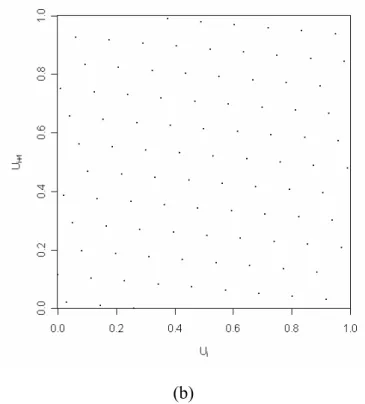
Xi = (25Xi – 1 + 7) mod 96, (3.10) Xi = (61Xi – 1 + 11) mod 96. (3.11)

Both of them have the full period, 96. Their means and variances are the same consequently. How to make selection between (3.10) and (3.11)? The pairs of consecutive numbers of these two LCGs are plotted in Figure 3.1:

(b)

Figure 3.1: The pairs of consecutive numbers of these two LCGs in (3.10) and (3.11)

are plotted in (a) and (b) respectively.

Ideally it is expected that these pairs of consecutive numbers should uniformly scatter in the unit square. In reality, these pairs fall on lattice structures as proved in Marsaglia (1968). Hence, one can examine the properties of lattice structures to select LCGs (Knuth 1998).

4. PARALLEL LINEAR RANDOM NUMBER GENERATORS

In order to accelerate the simulating time and improve efficiency, it is possible to parallelize the RNG with several computer processors. There are mainly two approaches to combine random numbers generated by different processors, sequence splitting and leapfrogging (Coddington, P. D. 1996). These two approaches will be discussed below.

4.1 Sequence Splitting

The generation of a total sequence of N random numbers is split by the random numbers generated by p processors. Suppose N = np and n is the number of random number that one process generates. The processor j, j = 1, 2, …, p, is responsible for producing the following random numbers in the total sequence:

X(j – 1)n + 1, X(j – 1)n + 2, …, Xjn (4.1)

4.2 Leapfrogging

The processor under the leapfrogging method generates random numbers in the total sequence with a lag of p. The system works like the allocation a deck of cards to

p players. The processor j, j = 1, 2, …, p, is responsible for producing the following

random numbers in the total sequence:

Xj, Xj + p, Xj + 2p, … (4.2)

5.

PARALLELIZATION WITH DIFFERENT INCREMENT

SHIFTS

For the LCG in (2.1), it is possible to consider the changing of a or c for different processor in parallel computing. This will be based on the lattice structures of LCGs as follows.

5.1 Minkowski Bases of the LCG

The Monkowski bases of the lattice structures for LCGs are shown in Marsaglia (1968). They are L = _{0 1 2} (5.1) 1 | , , , t i i t i V z V z z z = ⎧ + ⎨ ⎩

∑

V0 = 1 2 1 ( 1) 0, , (1 ) , (1 ) , , , 1 t c a c a c a a c m a − ⎛ _{+ + +} − ⎞ ⎜ ₋ ⎟ ⎝ … ⎠ V1 =

(

)

The increment c, simply showing up in V0, accounts for nothing but the shift of

lattice structure of an LCG. On the other hand, a does have a great effect on the shape of structure.

Moreover, (2.1) can be rewrite as composition of the equations below if c is smaller than m:

Xi = aXi – 1 + c, Xi = aXi – 1 + c – m, Xi = aXi – 1 + c – 2m,

Xi = aXi – 1 + c – (a – 1)m; (5.2)

or the followings if c is equal to or greater than m (which is often avoided):

Xi = aXi – 1 + c, Xi = aXi – 1 + c – m, Xi = aXi – 1 + c – 2m,

Xi = aXi – 1 + c – am. (5.3)

Apparently, the pair of consecutive numbers from LCGs will fall on few parallel lines. The parameter c shifts the lines while the parameter a changes the slope of them. If we choose c appropriately in the parallelization of LCGs, we can fill in the space between parallel lines in the lattice structure efficiently as illustrated in Figure 5.1. However, the changing of a in parallelization is very challenging because the shapes of lattices are changing accordingly. Hence, we will consider the parallelization of LCGs with different shift parameters in this study.

(a) (b)

(c) (d)

Figure 5.1: The lattice structures of parallel LCGs with different shift increments for

1 to 4 processors are illustrated in part (a) to (d).

Let Xi be the random sequence from the processor 1 and Yi be that from the

processor 2. Suppose that these two processors employ LCGs with the same a but different increments, c and c’. Then

Xi – Yi = [a(Xi – 1 – Yi – 1) + (c – c')] mod m (5.4) = ( _{0 0}) ( ')( 1) 1 i i c c a a X Y a ⎡ − − − + ⎢ ₋ ⎣ ⎦ ⎤ ⎥ mod m. (5.5) That is, Xi – Yi has its special lattice structure. It also implies that the random

sequence with leapfrogging method will follow a new lattice structure.

5.2 Parallel Design of Increment Shifts

Another reason for preferring c to a in parallelization is that given an LCG with a long period of m or m – 1, it is easy to find another c that yields the long period because it simply requires c be relatively prime to m. But the selection of a for parallelization for long period is very challenging.

To make the parallel design of increment shifts feasible for two processors, we consider: (1) (1) (1) (1) 1 (2) (2) (2) (2) 1 ( ) mod , / ; ( ) mod , ( 0.5) /( 0.5), (5.6) 2 , mod 1 0.5; where (( )) , mod 1 0.5. i i i i i i i i X aX c m U X m c m X aX m U X m y y y y y − − = + = ⎛⎛ + ⎞⎞ = +_{⎜⎜ ⎟⎟} = + + ⎝ ⎠ ⎝ ⎠ ⎧ ⎢ ⎥ ≥ ⎪ ⎣ ⎦ = ⎨ < ⎡ ⎤ ⎪ ⎢ ⎥ ⎩

The is calculated with the extra addition of 0.5 in both numerator and denominator because it can expand the outcome space. Most important of all, this extra addition ensures the absence of zero which is undesired for most of the practical applications. Also, addition in both numerator and denominator changes neither the mean nor the variance. It doesn’t draw different conclusions from

under the empirical tests either since there is merely a subtle change for the value of

(2) i U ( )j ( )j _/ i i U = X m ( )j i

Besides, some empirical tests consider only ( )j _, i

X which is not modified at all.

This idea can be extended to more than two processors. For three processors, we consider: (1) (1) (1) (1) 1 (2) (2) (2) (2) _{1 1} 3 3 1 (3) (3) (3) (3) _{2 2} 3 3 1 ( ) mod , / ; ( [ ]) mod , ( ) /( ); 3 2 ( [ ( ) ]) mod , ( ) /( ) (5 3 i i i i i i i i i i i i X aX c m U X m m c X aX c m U X m X aX c m c m U X m − − − = + = ⎛⎛ − ⎞⎞ = + +_{⎜⎜ ⎟⎟} = + + ⎝ ⎠ ⎝ ⎠ ⎛⎛ ⎞⎞ = + +_⎜⎜ − _⎟⎟ = + + ⎝ ⎠ ⎝ ⎠ .7)

For p processors, we consider:

( ) ( ) ( ) ( ) ( 1) ( 1) 1 ( [ ]) mod , ( ) /( ), j j j j j j p i i i i X aX c ε m U X − m − = + + = + + − p (5.8) where ε = j 1(m c) p ⎛_{⎛ −} ⎞ − ⎜⎜ ⎝ ⎠ ⎝ ⎠, ⎞ ⎟

⎟ j = 1, 2, …, p. If c + ε is not relatively prime to m, set ε = ε0, where ε0 is the nearest integer to ε that makes c + ε0 relatively prime to m.

Moreover, the Euclidean algorithm is capable of helping to check if c + ε0 is relatively

prime to m (Cormem, T. H., Leiserson, C. E., Rivest, R. L., and Stein, C. 2001). In practice, this check can be omitted since m is often chosen from prime numbers.

5.3 Serial Correlation

The quality of this kind of parallel RNG (PRNG) will be investigated. The uniformity, the expectation, and the variance are surely satisfactory. It is necessary to check the serial correlation. Let p be the number of processors. Following the similar steps from (3.3) to (3.5), we get the correlation for the sequence splitting methods as follows: RSS ≈ *( ) 1 1 2 ( , , ) 6 3 2 ( ) p p j j j j j j σ a m c p m X c p pm p = = ⎡ ⎤ ⎡ + − + + ⎢ ⎥ ⎢ ⎣ ⎦ ⎣ −

∑

∑

RSS ≈ 1 ( , , ) 6 p j j j σ a m c p pm = +

∑

∑

among processors with different cj. As a result, we go back to check the primitive

formula. If each processors generates the same amount of random numbers n, then:

RSS ≈ ( ) ( ) ( ) ( ) 1 1 1 1 1 1 1 1 2 2 ( ) 2 ( ) ( ) 2 ( ) 1 1 1 1 1 1 1 1 1 1 1 ( ) 1 1 ( ) ( ) p n p n p n j j j j i i i i j i j i j i p n p n p n p n j j j i i i i j i j i j i j i X X X X np X X X X np np + + = = = = = = + + = = = = = = = = − ⎛ ⎞ ⎛ ⎞ − _{⎜ ⎟} − _{⎜ ⎟} ⎝ ⎠ ⎝ ⎠

∑∑

∑∑

∑∑

∑∑

∑ ∑

∑∑

∑ ∑

∑∑

The equation of (5.13) is derived by using the fact that the sample mean and the sample variance of X(j) are approximately to 0.5p and

2

. 12

p

Then we get the bounds as following:

1min≤ ≤j pRj ≤ RSS ≤ 1max≤ ≤j pRj (5.14) Hence, the correlation of parallel LCGs by the sequence splitting method is

between the best and the worst correlation of p serial LCGs.

The serial correlation for the leapfrogging method RLF is difficult to obtain by

using the same idea from (3.3) to (3.5). We therefore directly check the primitive formula like (5.12): RLF = 1 ( ) ( 1) (1) ( ) ( ) ( ) 1 1 1 1 1 1 1 1 1 2 2 ( ) 2 ( ) ( ) 2 ( ) 1 1 1 1 1 1 1 1 1 1 1 ( ) ( ) 1 1 ( ) ( ) p n n p n n j j p j j i i i i i i j i i j i j i p n p n p n p n j j j i i i i j i j i j i j i X X X X X X np X X X X np np − + + + = = = = = = = + + = = = = = = = = ⎡ ⎤ + − ⎢ ⎥ ⎣ ⎦ ⎛ ⎞ ⎛ ⎞ − _{⎜ ⎟} − _{⎜ ⎟} ⎝ ⎠ ⎝ ⎠

∑∑

∑

∑∑

∑∑

∑∑

∑ ∑

∑∑

∑ ∑

RLF ≈ 1 ( ) ( 1) (1) ( ) 1 2 1 1 1 12 ( ) ( ) p n n j j p i i i i j i i X X X X m np − + + = = = ⎡ ⎤ 3 + − ⎢ ⎥ ⎣

∑∑

∑

serial correlation in (5.16) will decrease with the increase of N = np. The similar phenomenon can also be observed by the approximation of the serial correlation in (5.13). In practice, tremendous amount of random numbers is often generated in large simulation studies and the correlation will not be a major problem as illustrated in Figure 5.2.

(a) (b)

Figure 5.2: Serial correlations of the LCG with a = 16,807, c = 0, m = 231 – 1, and p =

4 in both (a) sequence splitting method and (b) leapfrogging method with the increasing of the number of random sequence generated. The absolute value of both correlations have been smaller than 0.01 when the number of output is greater than 15,000.

5.4 Lattice Structures

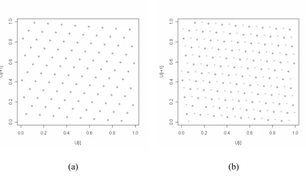
From the perspectives of uniformity and serial correlation, sequence splitting method and leapfrogging methods have compatible performances. But there is a great difference when they are compared on the plots of the pair of consecutive numbers. Take four processors as an example. The lattice structure of one LCG is plotted in Figure 5.3 (a). The lattice structure of parallel LCG by sequence splitting is plotted in Figure 5.3 (b), which shows the adding of three more sets of parallel lines. The lattice structure of parallel LCG by leapfrogging is plotted in Figure 5.3 (c), which shows more changes of lattice structures that could be useful to create more randomness.

(b) (c)

Figure 5.3: The lattice structure of the LCG, Xi = 16807Xi – 1 mod (231 – 1) is shown in

(a). Part (b) and (c) demonstrate the structures of the LCG mentioned-above with four processors and via sequence splitting method and leapfrogging method respectively.

5.5 Inter-processor Correlation

There may exist inter-processor correlation when applying the increment shift method for different processors. It might be expected that there exists highly positive correlation when the initial seeds are the same and the differences among the increments are very small.

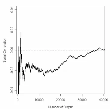
For illustration, we simulate pseudo random numbers with the parallel LCG set, and (1) (1) 31 1 16807 mod (2 1) i i X = X ₋ − (2) (2) 31 1 (16807 1) mod (2 1) i i X = X₋ + − using leap- frogging method. Both initial seeds of these two LCGs are set to 1. The scatter plot is shown in Figure 5.4. The serial correlation is plotted in Figure 5.5. There does not seem to have high inter-correlation even when the initial seeds are the same and the differences among the increments are very small.

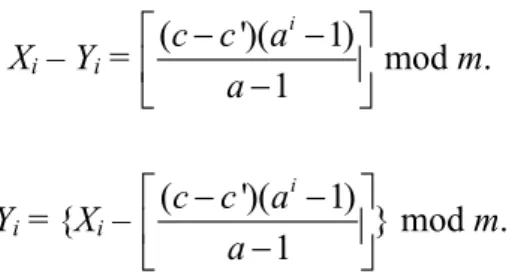
then we can simplify the equation into Xi – Yi = ( ')( 1) 1 i c c a a ⎡ − − ⎤ ⎢ ₋ ⎥ ⎣ ⎦mod m. (5.18) Yi = {Xi – ( ')( 1) } 1 i c c a a ⎡ − − ⎤ ⎢ ₋ ⎥ ⎣ ⎦ mod m. (5.19) This shows the random sequence still possesses a new lattice structure even without the term of ai(X0 – Y0). Namely, the scatter plot of (Xi, Yi) or that of

in Figure 5.3 does never appear with a highly correlated pattern, say, a line. The serial correlation

(1) (2)

(X_i ,X )_i

Figure 5.4: Scatter plot for the pair of is shown for the parallel LCG set,

and (1) (2) (Xi ,X )i (1) (1) 31 1 16807 mod (2 1) i i X = X ₋ − (2) (2) 31 1 (16807 1) mod (2 1). i i X = X₋ + −

Figure 5.5: Serial correlations of this parallel LCG set with leapfrogging method. The

correlation is desirably small especially when the number of pseudo-random number generated is larger than 25,000.

5.6 Absorbing States

It is aimed to parallelize the multiplicative LCGs that can attain the maximum periods. Each processor of the multiplicative LCG yields random numbers with a period of m – 1. It is evident that 0 is an absorbing state of the multiplicative LCG that is not desired. If the initial seed is the absorbing seed of 0, then the multiplicative LCG will enter the absorbing state of 0. The absorbing states and seeds shall be avoided in the parallelization of RNGs.

For the increment c in (2.1) ≠ 0, we can figure out the absorbing states and seeds by means of the extended Euclidean algorithm in the followings. Let Xa denote as the

absorbing seed, then we can rewrite (2.1) into (5.20) and (5.21):

Xa = (aXa + c) mod m; (5.20)

As c < m, we can simplify (5.21) as follows:

(a – 1)Xa mod m = m – c. (5.22)

Then it becomes the question of solving the linear congruence.

Firstly, we consider a linear congruence of Ax mod M = 1. We can find an integer

k such that

Ax – kM = 1. (5.23)

If y = –k,

Ax + My = 1 (5.24)

Through the extended Euclidean algorithm (Cormem, T. H., Leiserson, C. E., Rivest, R. L., and Stein, C. 2001), we are able to obtain one of the solutions, say (x0, y0).

Next, we try to solve Ax mod M = B. In the beginning, we multiply B in the equation Ax mod M = 1 and substitute the solution x0 into it:

B(Ax0 mod M) = B; (5.25)

(B mod M)(Ax0 mod M) = B; (5.26) A(Bx0) mod M = B. (5.27) Then, it is clear that Bx0 satisfies the linear congruence Ax mod M = B. The same idea

goes in (5.22). For the purpose of figuring out Xa, we can employ the extended

Euclidean algorithm to find out α0 in (5.28).

(a – 1)α0 + mβ0 = 1. (5.28)

In order to ensure that the absorbing seed is smaller than m, we let

Xa = [α0 ×(m – c)] mod m. (5.29)

Since we can calculate the absorbing seeds, we ought to avoid them in advance. Obviously, the more processors are hired, the more starting values should be avoided.

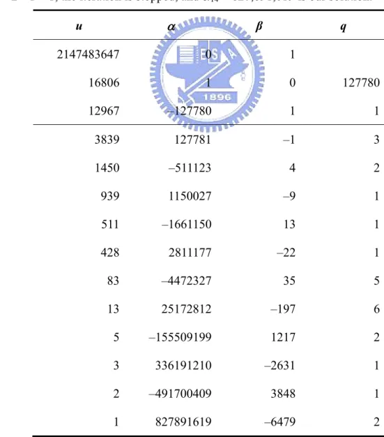
Table 5.1: An example of a = 16,807 and m = 231 – 1 to illustrate the implementation

of the algorithm via the iterative method.

u1 = m = 231 – 1, u2 = a – 1 = 16806,

α1 = 0, α2 = 1, β1 = 1, β2 = 0, qi = ⎢⎣ui−1/ui⎥⎦ i = 2, 3, … ,

uj = uj – 2 – uj – 1 ×qj – 1 αj = αj – 2 – αj – 1 ×qj – 1 βj = βj – 2 – βj – 1 × qj – 1, j = 3, 4, …

Repeat the computation until uj = 1. The last αj is the solution, α0 in (5.28).

For example, q2 = ⎢_⎣(231−1) /16806⎥⎦ = 127,780, u3 = (231 – 1) – 16806×127780

= 12,967, α3 = 0 – 1×127780 = –127,780, β3 = 1 – 0×127780 = 1, … Because u14 =

3 – 2×1 = 1, the iteration is stopped, and α14 = 827,891,619 is our solution.

u α β q 2147483647 0 1 16806 1 0 127780 12967 –127780 1 1 3839 127781 –1 3 1450 –511123 4 2 939 1150027 –9 1 511 –1661150 13 1 428 2811177 –22 1 83 –4472327 35 5 13 25172812 –197 6 5 –155509199 1217 2 3 336191210 –2631 1 2 –491700409 3848 1 1 827891619 –6479 2

From Table 5.1, we get α0 = α14 = 827,891,619, and the absorbing seed is:

Xa = [827891619×(231 – 1 – c)] mod (231 – 1) (5.30)

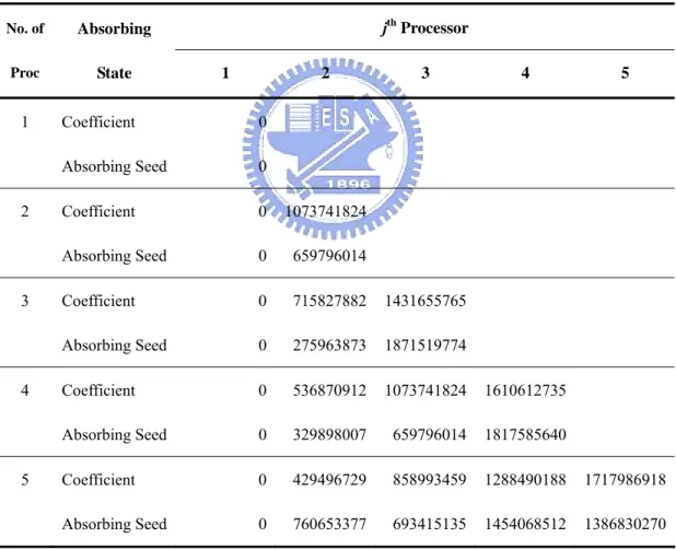
Table 5.2: The table shows the parallel LCG set with a = 16,807 and m = 231 – 1 with

processors varied from one to ten. For instance, for 3 processors, the parallel LCG set will be (1) (1) 31 (2 1 16807 mod (2 1), i i X = X₋ − (2) (2) 1 (16807 715827882) mod i i X = X₋ + 31 _–

1), and The absorbing state occurs at 0, 275,963,873, and 1,871,519,774, respectively. (3) (3) 1 (16807 1431655765) mod. i i X = X ₋ + jth Processor No. of Proc Absorbing State 1 2 3 4 5 1 Coefficient 0 Absorbing Seed 0 2 Coefficient 0 1073741824 Absorbing Seed 0 659796014 3 Coefficient 0 715827882 1431655765 Absorbing Seed 0 275963873 1871519774 4 Coefficient 0 536870912 1073741824 1610612735 Absorbing Seed 0 329898007 659796014 1817585640 5 Coefficient 0 429496729 858993459 1288490188 1717986918 Absorbing Seed 0 760653377 693415135 1454068512 1386830270

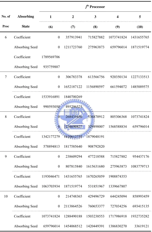
Table 5.2 (Continued) jth Processor 1 2 3 4 5 No. of Proc Absorbing State (6) (7) (8) (9) (10) 6 Coefficient 0 357913941 715827882 1073741824 1431655765 Absorbing Seed 0 1211723760 275963873 659796014 1871519774 Coefficient 1789569706 Absorbing Seed 935759887 7 Coefficient 0 306783378 613566756 920350134 1227133513 Absorbing Seed 0 1652187122 1156890597 661594072 1485889575 Coefficient 1533916891 1840700269 Absorbing Seed 990593050 495296525 8 Coefficient 0 268435456 536870912 805306368 1073741824 Absorbing Seed 0 1238690827 329898007 1568588834 659796014 Coefficient 1342177279 1610612735 1879048191 Absorbing Seed 578894813 1817585640 908792820 9 Coefficient 0 238609294 477218588 715827882 954437176 Absorbing Seed 0 807815840 1615631680 275963873 1083779713 Coefficient 1193046471 1431655765 1670265059 1908874353 Absorbing Seed 1063703934 1871519774 531851967 1339667807 10 Coefficient 0 214748365 429496729 644245094 858993459 Absorbing Seed 0 2113864526 760653377 727034256 693415135 Coefficient 1073741824 1288490188 1503238553 1717986918 1932735282 Absorbing Seed 659796014 1454068512 1420449391 1386830270 33619121

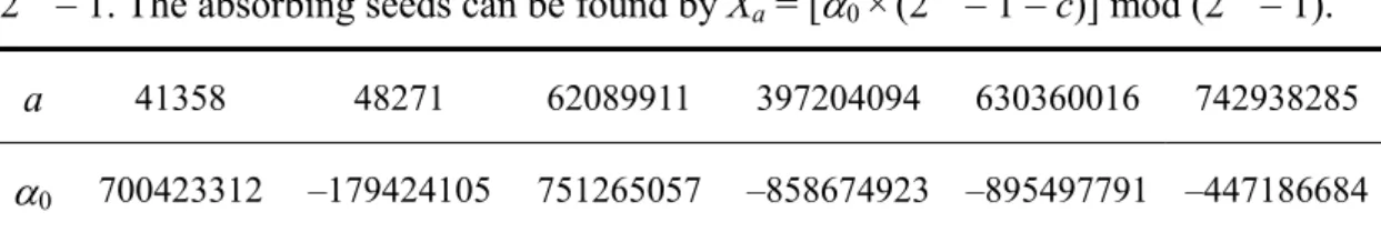
Table 5.3: List of α0’s for some other popular multipliers with the same modulus =

231 – 1. The absorbing seeds can be found by Xa = [α0 ×(231 – 1 – c)] mod (231 – 1). a 41358 48271 62089911 397204094 630360016 742938285

α0 700423312 –179424105 751265057 –858674923 –895497791 –447186684

Table 5.2 shows different absorbing seeds for the parallel LCG set with a = 16,807 and m = 231 _{– 1 under different processors. Via the same algorithm, absorbing}

states of other popular LCGs are listed in Table 5.3.

The increment shift method can also extend to the MRG case because (2.3) is able to be rewritten as composition of some parallel hyperplanes like (5.2) and (5.3). The parameter c only shifts this planes. Consequently, we now add the increment c in (2.3):

Xi = (a1Xi – 1 + a2Xi – 2 +…+ akXi – k + c) mod m (5.31)

If the generator enters the absorbing state, the output vector (Xi – k, Xi – k + 1, …, Xi – 1) and the next one (Xi – k + 1, Xi – k + 2, …, Xi ) are suppose to be the same. It only

occurs when Xi – k = Xi – k + 1 =…= Xi – 1 = Xi. In other words, the absorbing state arises

when the initial vector is (Xa, Xa, …, Xa). Therefore, we can solve out the absorbing

seed by replacing all Xi’s with Xa:

Xa = (a1Xa + a2Xa +…+ akXa + c) mod m (5.32) ( – 1) mod m = m – c (5.33) 1 k k a i a X =

∑

Now it turns into the question concerning the linear congruence again. But the equation changes from (5.27) into (5.34).

( 1 k k i a =

∑

6. SIMULATION RESULT

First we study the parallel LCG with a = 16,807 and m = 231 – 1. One billion pseudo-random numbers are generated with ten different seeds and processors by leapfrogging method. We employ DIEHARD tests which contains 17 test sets and 269

p-values (Marsaglia, G. 1995 and Gentle, J. E. 2003). Besides, α = 0.01 and 0.05 are chosen as the threshold of the p-values.

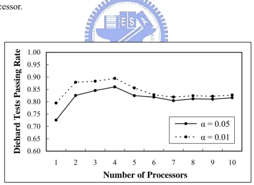
Figure 6.1 illustrates the average passing rate of 269 p-values from ten different initial seeds with different parameters. From only one processor to two, the performance of the parallel LCG greatly improves. It keeps improving until p = 4 and then falls back around 80% – but the performances are still better than that by only one processor. 0.60 0.65 0.70 0.75 0.80 0.85 0.90 0.95 1.00 1 2 3 4 5 6 7 8 9 10 Number of Processors Die h ar d Te st s Passing Rat e α = 0.05 α = 0.01

Figure 6.1: Passing rate of the DIEHARD test for the parallel LCG with a = 16,807

and m = 231 – 1. Processors varied from one to ten are tested and the threshold α = 0.01 and 0.05 are used. Ten different initial seeds are make and averaged to calculate the passing rate.

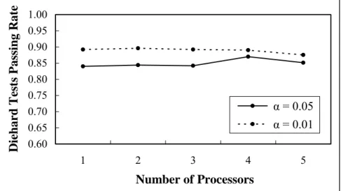
Next, we check the MRG of DX-1597-4 in (2.12). For the purpose of avoiding the problem of overfloating, Jean-Louis (2005) suggest the change of (2.12) to (6.1) in programming:

Xi = 29,746[36,097(Xi – 1 + Xi – 533 + Xi – 1065 + Xi – 1597) mod (231 – 1)] mod (231 – 1).

(6.1) The same test package is employed to study this parallel generator. First, it is obvious that the MRG pass more tests than the LCG. The simulation result gives the similar results that the number of processors is suggested to be two or four. Additionally, Since the original MRG (with p = 1) has passed many tests, more processors don’t do much improvement in this case.

0.60 0.65 0.70 0.75 0.80 0.85 0.90 0.95 1.00 1 2 3 4 5 Number of Processors D

iehard Tests Passing Rate

α = 0.05 α = 0.01

Figure 6.2: Passing rate of the DIEHARD test for the parallel MRG of DX-1597-4 in

(2.12). Processors varied from one to five are tested and the threshold α = 0.01 and 0.05 are used. Two different initial seeds are make and averaged to calculate the passing rate.

7. CONCLUSION AND DISCUSSION

We have proposed a simple and effective approach to parallelize linear RNGs with different increment shifts, including LCGs and MRGs. The implementation of

this kind of parallel RNGs is easy and the improvements are as expected. Theoretic and simulation investigations are performed to confirm this new proposal.

There are two major approaches to connect random numbers generated by different processors, sequence splitting and leapfrogging. From the properties of lattice structure, the leapfrogging method dominates in the simulation studies. Also, theoretically, the leapfrogging method yields the much better lattice structure than the sequence splitting.

In particular, we examine the parallel LCG with a = 16,807 and m = 231 – 1 through simulation tests. On the average, it performs best when p = 4 among 1 to 10 processors. It is interesting to perform more investigation to explore more about this phenomenon. More studies are of interest to pursuit in the future to understand the properties of this kind of parallel linear RNGs.

REFERENCES

[1] Alanen, J. D. and Knuth D. E. (1964), “Tables of Finite Fields,” Sankhyā A, 26, 305-328

[2] Bratley, P., Fox, B. L., and Schrage, L. E. (1987), A Guide to Simulation (2nd ed). New York: Springer.

[3] Bishop M. (2002), Computer Security: Art and Science (1st ed). Massachusetts: Addison-Wesley.

[4] Coddington, P. D. (1996), “Random Number Generators for Parallel Computers,” NHSE Review 1996 Volume, Second Issue.

[5] Cormem, T. H., Leiserson, C. E., Rivest, R. L., and Stein, C. (2001),

Introduction to Algorithm (2nd ed). Massachusetts: MIT Press.

[6] Dagpunar, J. (1988), Principles of Random Variate Generation (1st ed). Oxford, U.K.: Clarendon Oxford Science Publications.

[7] Deng, L. Y. (2005), “Efficient and Portable Multiple Recursive Generators of Large Order,” ACM Transactions on Modeling and Computer Simulation 15, 1. [8] Deng, L. Y. and Lin, D. K. J. (2000), “Random Number Generation for the New

Century,” American Statistician 54, 2, 145-150.

[9] Deng, L. Y. and Xu, H. Q. (2003), “A System of High-Dimensional, Efficient, Long-cycle and Portable Uniform Random Number Generators,” ACM

Transactions on Modeling and Computer Simulation 13, 4, 299-309.

[10] Foulley, J. L. (2005), “Multiple Recursive Random Number Generators and their APL Programmes,” Technical Report, INRA-SGQA, 14

[11] Gentle, J. E. (2003), Random Number Generation and Monte Carlo Methods (2nd ed). New York: Springer.

[12] Knuth, D. E. (1998), The Art of Computer Programming, Volume 2:

[13] Law, A. M. and Kelton, W. D. (2000), Simulation Modeling and Analysis (3rd ed). New York: McGraw-Hill.

[14] L’Ecuyer, P. (1990), “Random Numbers for Simulation,” Communications of the

ACM 33, 85-98.

[15] L’Ecuyer, P. (1997), “Bad Lattice Structures for Vectors of Non-Successive Values Produced by Some Linear Recurrences,” INFORMS Journal on

Computing 9, 57-60.

[16] L’Ecuyer, P. (1998), “Random Number Generation,” Handbook on Simulation:

Principles, Methodology, Advances, Applications, and Practice (1st ed). Banks, J., ed. New York: Wiley.

[17] L’Ecuyer, P. (1998), “Uniform Random Number Generators,” Proceedings of the

1998 Winter Simulation Conference, IEEE Press

[18] L’Ecuyer, P. (2004), “Random Number Generation,” Handbook of

Computational Statistics (1st ed). Gentle, J. E., Härdle, W., and Mori, Y., eds. New York: Springer

[19] L’Ecuyer, P. (2006), “Uniform Random Number Generation,” Handbooks in

Operations Research and Management Science: Simulation (1st ed). Henderson, S. G. and Nelson, B. L., eds. Amsterdam, Holland: Elsevier Science.

[20] L’Ecuyer, P., Blouin, F., and Couture, R. (1993), “A Search for Good Multiple Recursive Random Number Generators,” ACM Transactions on Modeling and

Computer Simulation 3, 2, 87-98.

[21] Lehmer, D. H. (1951), “Mathematical methods in large-scale computing units,”

Proceedings of the Second Symposium on Large Scale Digital Computing Machinery, 141-146, Massachusetts: Harvard University Press.

[22] Marsaglia, G. (1968), “Random Numbers Fall Mainly in the Planes,”

Proceedings of the National Academy of Sciences of the United States of America 61, 1, 25-28

[23] Marsaglia, G. (1995), The Marsaglia Random Number CDROM including the

Diehard Battery of Tests of Randomness, Department of Statistics, Florida State

University, Tallahassee, Florida, Available at http://www.csis.hku.hk/~diehard/cdrom.

[24] Mascagni, M. (1998), “Parallel Linear Congruential Generators with Prime Moduli,” Parallel Programming 24, 923-926.

APPENDIX

Table A1: Summary results of DIEHARD test for the parallel LCG with a = 16,807,

m = 231 – 1, and the number of processors p varied from one to ten. The threshold α = 0.01 and 0.05 are set to calculate the passing rate of the LCG. Ten different initial seeds X0’s are used and the results are averaged to plot the Figure 6.1.

1 214748365 429496729 644245094 858993458 Seed No of p 0.05 0.01 0.05 0.01 0.05 0.01 0.05 0.01 0.05 0.01 1 0.7212 0.7918 0.7138 0.7955 0.7398 0.7993 0.7249 0.7955 0.7361 0.8030 2 0.8625 0.8959 0.8699 0.9071 0.8067 0.8848 0.7435 0.8290 0.8141 0.8587 3 0.8364 0.8810 0.8327 0.8699 0.8104 0.8736 0.8401 0.8699 0.8550 0.8848 4 0.8662 0.8996 0.8736 0.8996 0.8662 0.8922 0.8550 0.8959 0.8513 0.8959 5 0.8327 0.8625 0.8141 0.8476 0.8253 0.8587 0.8253 0.8550 0.8290 0.8587 6 0.8216 0.8253 0.8141 0.8290 0.8216 0.8290 0.8216 0.8327 0.8216 0.8290 7 0.8104 0.8216 0.7993 0.8141 0.7993 0.8141 0.8067 0.8178 0.8067 0.8216 8 0.8104 0.8253 0.8067 0.8253 0.8141 0.8253 0.8141 0.8216 0.8067 0.8253 9 0.8104 0.8216 0.8104 0.8253 0.7993 0.8141 0.8104 0.8216 0.8141 0.8178 10 0.8141 0.8253 0.8141 0.8290 0.8178 0.8290 0.8178 0.8290 0.8216 0.8290 1073741823 1288490188 1503238552 1717986917 1932735281 Seed No of p 0.05 0.01 0.05 0.01 0.05 0.01 0.05 0.01 0.05 0.01 1 0.7100 0.7807 0.7323 0.7955 0.7249 0.7955 0.7286 0.7993 0.7249 0.7918 2 0.8141 0.8810 0.8513 0.8922 0.8253 0.8736 0.8439 0.8922 0.8253 0.8773 3 0.8699 0.8922 0.8699 0.8996 0.8178 0.8885 0.8550 0.8810 0.8662 0.8922 4 0.8587 0.8959 0.8550 0.8922 0.8625 0.8922 0.8699 0.8959 0.8439 0.8885 5 0.8290 0.8550 0.8178 0.8550 0.8178 0.8476 0.8253 0.8550 0.8327 0.8625 6 0.8216 0.8290 0.8253 0.8253 0.8104 0.8290 0.8178 0.8290 0.8141 0.8253 7 0.7993 0.8178 0.8030 0.8178 0.8067 0.8216 0.8104 0.8253 0.8030 0.8216 8 0.8141 0.8253 0.8104 0.8216 0.8141 0.8290 0.8104 0.8216 0.8178 0.8253 9 0.8178 0.8253 0.8104 0.8216 0.8067 0.8253 0.8141 0.8253 0.8104 0.8253 10 0.8178 0.8253 0.8178 0.8290 0.8141 0.8253 0.8141 0.8290 0.8141 0.8253

Table A2: Summary results of DIEHARD test for the parallel MRG of DX-1597-4 in

(2.12), and the number of processors p varied from one to five. The threshold α = 0.01 and 0.05 are set to calculate the passing rate of the MRG. Two initial seeds X0’s are

used and the results are averaged to plot the Figure 6.2.

1 1073741823 Seed No of p 0.05 0.01 0.05 0.01 1 0.8364 0.8959 0.8439 0.8885 2 0.8476 0.8922 0.8401 0.8996 3 0.8364 0.8885 0.8476 0.8959 4 0.8699 0.8885 0.8699 0.8922 5 0.8476 0.8699 0.8550 0.8810