單一頻道之無線近身網路合併設計

國立交通大學

電子工程學系

電子研究所

碩 士 論 文

單一頻道之無線近身網路合併設計

Single Channel Network Merging for Wireless

Body Area Network

研 究 生：李英昌

指導教授：黃經堯 教授

單一頻道之無線近身網路合併設計

Single Channel Network Merging for Wireless

Body Area Network

研 究 生：李英昌 Student: Ying-Chang Li

指導教授：黃經堯 Advisor: ChingYao Huang

國 立 交 通 大 學

電 子 工 程 學 系

電 子 研 究 所

碩 士 論 文

A Thesis

Submitted to Department of Electronics Engineering College of Electrical & Computer Engineering

National Chiao Tung University in Partial Fulfillment of the Requirements

for the Degree of Master

in

Electronics Engineering July 2010

Hsinchu, Taiwan, Republic of China

i

單一頻道之無線近身網路合併設計

學生：李英昌

指導教授：黃經堯 教授

國立交通大學電子工程學系電子研究所

摘 要

ii

Single Channel Network Merging for Wireless

Body Area Network

Student: Ying-Chang Li

Advisor: Ching-Yao Huang

Department of Electronics Engineering

National Chiao Tung University

ABSTRACT

For the low power consumption requirement of WBAN, we analyze the advantages and disadvantages of the existing systems and propose a TDMA based network merging control method to reduce the interference between the networks. It might achieve the low power consumption requirement of sensor nodes. In addition to proving the simulations, we implement this method on the transmission module to test the effect of the actual operation.

iii

誌 謝

iv

目 錄

Chapter 2. Overview of 802.11 MAC Protocol ...3

2.1. Fundamentals of 802.11 ...3

2.2. MAC Protocol Structure ...3

2.2.1. CSMA/CA Mechanism ...4

2.2.2. RTS/CTS Mechansim ...4

2.3. Power Consumption for WBAN ...6

2.4. Simulation ...8

2.4.1. Simulation Setup ...8

2.4.2. 802.11 MAC Simulation Result ...8

Chapter 3. Beacon Period Table Based Protocol ... 11

3.1. System Architecture ... 11

3.1.1. Beacon Period Table ... 11

3.1.2. Transmission Behavior ...13

3.2. Scenario...16

v

3.2.2. Multiple Users Environment ...17

3.3. Simulation ...18

3.3.1. Simulation Setup ...18

3.3.2. Beacon Period Table Based Protocol Simulation Result ...19

Chapter 4. Implementation on TinyOS ...21

4.1. TinyOS and Transmission Module Introduction ...21

4.2. MAC Architecture ...22

4.2.1. Frame Type ...22

4.2.2. CPN Architecture ...24

4.2.3. WSN Architecture ...28

4.3. Power Consuption Analysis ...32

4.3.1. Environment Setting ...32

4.3.2. Power Measurement...34

Chapter 5. Conclusion ...38

vi

表 目 錄

Table 1: The size and transmission time of the frames ...8

Table 2: An example of Beacon Period Table ...13

Table 3: The size and transmission time of the frames ...19

Table 4: Values of the frame type subfield ...22

vii

圖 目 錄

Figure 1: Schematic diagram of single user and whole system environment ...2

Figure 2: An example of RTS/CTS mechanism and CSMA/CA ...6

Figure 3: State diagram of RTS/CTS mechanism and CSMA/CA ...6

Figure 4: Network topology ...7

Figure 5: Idle listening problem schematic diagram...7

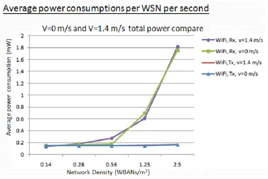
Figure 6: Average power consumptions per WSN per second ...9

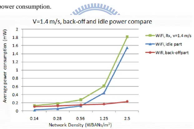
Figure 7: V=1.4m/s, the resource of Rx part power consumption compare ...10

Figure 8: Fixed beacon interval problem ...12

Figure 9: Random beacon interval ...12

Figure 10: WSN state diagram ...15

Figure 11: Single user environment timing diagram ...17

Figure 12: Multiple users environment timing diagram ...18

Figure 13: Average power consumptions per WSN per second ...20

Figure 14: Beacon period table and 802.11 MAC protocol Rx power of WSN compare ...20

Figure 15: The components of transmission module ...22

Figure 16: CPN architecture blocking diagram ...24

Figure 17: Command Manager blocking diagram ...25

Figure 18: Beacon Generator blocking diagram ...27

Figure 19: WSN architecture blocking diagram ...28

Figure 20: Command Management and Beacon Management blocking diagram ...30

Figure 21: Schematic diagram of Data Buffer and Data Control ...31

Figure 22: Control Unit blocking diagram...32

Figure 23: Network merging scenario ...33

viii

Figure 25: The circuit of ZXCT1010 with the transmission module ...34 Figure 26: The current consumption of WSN in one cycle ...35

ix

符 號 與 略 語 說 明

略 語 說 明

WBAN Wireless Body Area Network

CPN Central Process Node

WSN Wireless Sensor Node

DCF Distributed Coordination Function

PCF Point Coordination Function

CSMA/CA Carrier Sense Multiple Access and Collision Avoid

RTS/CTS Request to Send / Clear to Send

NAV Network Allocation Vector

MAC Medium access control layer

1

Chapter 1 Introduction

Wireless Body Area Network [1] (WBAN) is the network formed by the nodes which are used to sense human physiological signal. Because most sensor nodes are difficult to change or recharge the batteries, the nodes should work long enough without intervention. Therefore, the main requirement of WBAN is the power efficiency. To achieve the power efficiency, we could start from reducing the probability of transmission collision and reducing the idle receiving time.

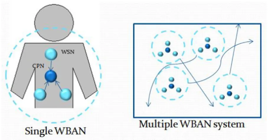
WBAN system model is shown in Figure 1. The whole WBAN topology is a hybrid network which consists of the following two types: 1. Single WBAN

Single WBAN is deployed as a star topology that is made up of one Central Process Node (CPN) and multiple Wireless Sensor Nodes (WSNs). CPN is used to coordinate the data transmission time of WSNs and receive the data frames from WSNs. WSN is used to sense human physiological signal and transmits that to CPN.

2. Multiple WBANs

The multiple WBAN system consists of several WBANs. It is a distributed topology which has no higher controller and no global knowledge.

Due to all networks use the same single channel, when people who use the WBAN services start moving, the networks will interfere each other and cause the frames collision and retransmission [2]. If we don’t use the appropriate mechanism to schedule the transmission time of each network,

2

the inter-network interference will increase the power consumption.

Figure 1: Schematic diagram of single user and whole system environment

The existing systems providing healthcare services are Bluetooth [3] and Zigbee [4]. Bluetooth uses frequency hopping over 79 channels to reduce the interference between each other. Zigbee uses CSMA/CA mechanism to solve this problem. However, with the increasing of network density, those systems still have difficulties in handling the interference in the single channel scenario. Therefore, we propose a network merging method for the single channel WBAN. This method might reduce the collision probability and the idle receiving time of the transceivers so that the power consumption of the sensor nodes could be reduced.

The thesis is organized as follows: Chapter 2, we introduce the protocol of IEEE 802.11 MAC protocol. Chapter 3, we propose a network merging protocol for WBAN system. Chapter 4, we show how to implement this protocol on TinyOS. Finally, we conclude our work in Chapter 5.

3

Chapter 2 Overview of 802.11 MAC Protocol

IEEE 802.11 MAC protocol is one of the most common protocols. This chapter will introduce IEEE 802.11 MAC architecture [5,6] and its collision avoidance mechanism. However, this protocol seems had power consumption issue for WBAN.

2.1 Fundamentals of 802.11

IEEE 802.11 MAC provides two main functions of access channel: Distributed Coordination Function (DCF) and Point Coordination Function (PCF). “Coordination Function” is a mechanism which determined when a device can start sending data. DCF is the basic access method which is mainly used Carrier Sense Multiple Access and Collision Avoid (CSMA/CA) technology to provide non-synchronize data transmission. This method can be used in distributed topology system like the whole WBAN topology. PCF provides a contention free method, and therefore doesn’t occur frame collision situations. However, PCF can only be used with the wireless infrastructure network. For WBAN MAC design, we will focus on DCF using.

2.2 MAC Protocol Structure

Carrier sensing is used to determine whether the transmission medium is in available state. IEEE 802.11 provides two carrier sensing functions: Physical Carrier-Sensing and Virtual Carrier-Sensing. As long as one of the sensing functions detects the channel state is busy,

4

MAC will return this situation to upper layer.

2.2.1 CSMA/CA Mechanism

By using CSMA/CA technology, different devices can share the same transmission medium, and avoid the possible transmission collision between different devices. CSMA/CA is used carrier sensing technology to measure the signal energy of current channel and determine whether the signal energy reaches a point of reference. If the signal strength is below this reference point, it means current channel is idle. If the signal strength is above the reference point, said the channel is busy. In this case, the devices need to wait a random back-off time. After the waiting time, the devices detect channel state again. This mechanism is through detecting channel and random delays to stagger the transmission time of different devices and reduce collisions.

2.2.2 RTS/CTS Mechanism

RTS/CTS (Request to Send / Clear to Send) mechanism is used to reduce frame collisions introduced by the hidden terminal problem. The flow is as following: Before the transmitter sends data frames, it will send a RTS frame to receiver. When the receiver receives the RTS frame, it will send back a CTS frame to confirm the request. Only when the transmitter receives the reply message, which implies that the RTS collision did not occur, the transmitter can send data frames. Simultaneously, when other devices receive these two control frames, they will stop trying to send frames temporarily. Therefore, the possibility

5

of frame collision between the transmitter and other devices will greatly reduce.

In IEEE 802.11, how long should other devices stop trying to transmit is determined by Network Allocation Vector (NAV). RTS frame and CTS frame contain information about the frame sending duration. When other devices hear the transmitter sends RTS frame or receiver sends CTS frame, they will record the duration in their Network Allocation Vector. This way, before NAV counts down to zero, it means that the device can’t send frames because the channel is in busy state now. Network Allocation Vector is like carrier vector detection. It can tell the device whether the transmission medium is busy, so it referred as Virtual

Carrier-Sensing Method.

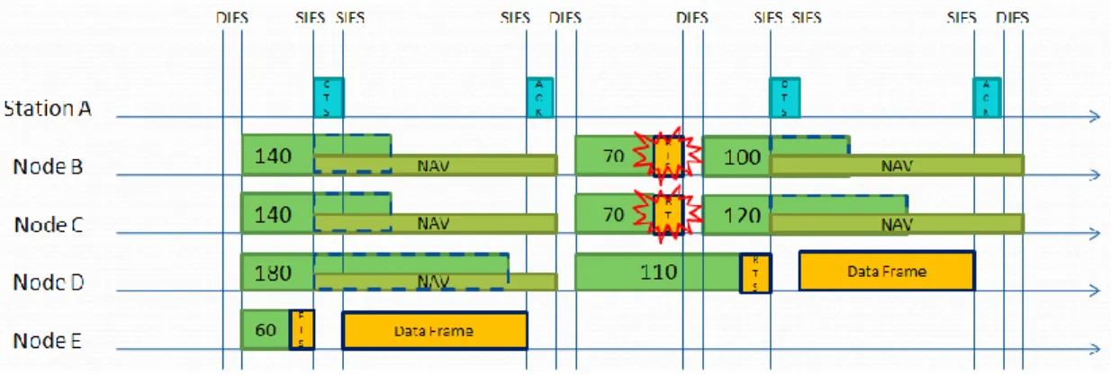
There is an example of RTS/CTS mechanism and CSMA/CA shown in Figure 2. Node B~E wanted to transmit data to Station A. First, they shall wait for a random back-off time: Node B was 140, Node C was 140, Node D was 180 and Node E was 60. When Node E counted down completed, it sent RTS frame to Station A and waited for the replied CTS frame. Other Nodes which heard this RTS or CTS frame recorded the duration in their NAV and stopped counting the back-off time. After the NAV finished, they will continue to count down the back-off time. The state diagram and the power level of each state are presented in Figure 3.

6

Figure 2: An example of RTS/CTS mechanism and CSMA/CA

Figure 3: State diagram of RTS/CTS mechanism and CSMA/CA

2.3 Power Consumption for WBAN

For WBAN, the NAV information has been used for power saving. When a device’s NAV is not equal to zero, it means the channel is in a busy state now. For power saving purpose, the transceiver of this device will go into sleep mode until NAV counts down to zero.

However, the effect of this power-saving function might be degraded with the increasing of the WBAN density. A schematic diagram is

7

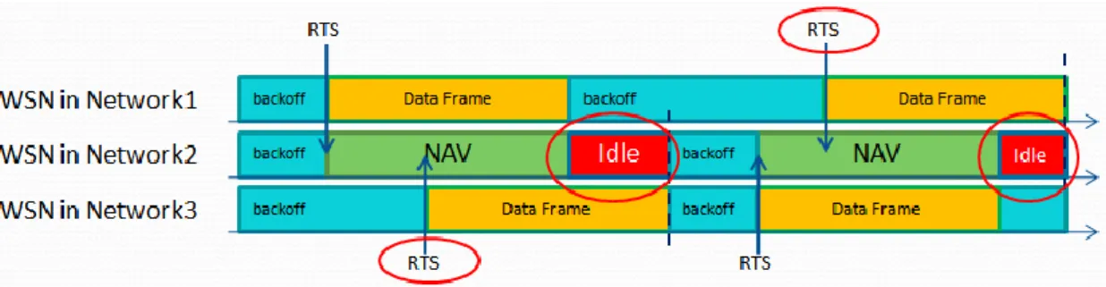
depicted in Figure 4, when a WSN in Network1 sent a RTS frame and transmitted its data, the WSNs in Network2 recorded this duration in their NAV and then entered the sleep mode. During the NAV duration, a WSN in Network3 also sent a RTS frame. The WSNs in Network2 would miss this RTS frame because they were in sleep mode. After the NAV duration finished, the WSNs in Network2 would stay in idle state until the WSN in Network3 finished its data transmission. This situation is shown in Figure 5. And with the increasing of network density, the incidence of this situation might increase significantly. It’s the reason that the effect of this power-saving function might decrease with the increasing of the WBAN density. The simulation of power consumption will be presented in section 2.4.

Figure 4: Network topology

8

2.4 Simulation

2.4.1 Simulation Setup

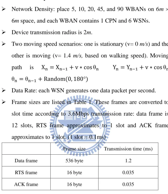
 Network Density: place 5, 10, 20, 45, and 90 WBANs on 6m × 6m space, and each WBAN contains 1 CPN and 6 WSNs.

 Device transmission radius is 2m.

 Two moving speed scenarios: one is stationary (v= 0 m/s) and the other is moving (v= 1.4 m/s, based on walking speed). Moving path is

 Data Rate: each WSN generates one data packet per second.  Frame sizes are listed in Table 1. These frames are converted to

slot time according to 3.6Mbps transmission rate: data frame is 12 slots, RTS frame approximates to 1 slot and ACK frame approximates to 1 slot. (1 slot = 0.1ms)

Frame size Transmission time (ms)

Data frame 536 byte 1.2

RTS frame 16 byte 0.035

ACK frame 16 byte 0.035

Table 1: The size and transmission time of the frames

 Back-off parameters are set to typical values: CWmin=15 slots, CWmax=1023 slots.

 The transceiver Tx and Rx mode power set to equal. The operating voltage is 3V and the current of Tx/Rx mode is 38.2mA.

9

2.4.2 802.11 MAC Simulation Result

For WSNs, the power consumption can be divided into Rx part and Tx part. The Rx part contains back-off and idle. The Tx part contains data frame and RTS frame transmission. The relationship between the state and power consumption can refer to Figure 3 at Section 2.2.2.

The average power consumption of WSN in stationary and mobile state is presented in Figure 6. The total power consumption hardly has any difference between stationary and mobile states. The probability of transmission collision does not increase when network is moving. Therefore, 802.11 MAC protocol is good at adaptation for mobility and suitable for the characteristic of WBAN transmits in mobile. However, compared with Tx power, we found that Rx power is OK at low network density, but it increases significantly with the increase of network density. The power of Rx part accounts for a large proportion of total power consumption.

10

We divided Rx power into idle part and back-off part to see what cause the Rx power to increase. As shown in Figure 7, we found that the idle part power is the main factor for the increase of Rx power. The reason of high power consumption of idle part has been explained at Section 2.3. Because WSNs enter the sleep mode, they will miss the RTS frame. After the NAV duration finishes, the WSNs stay in idle state until other networks finish their data transmission. And with the increasing of network density, the incidence of this situation increase significantly. Therefore, the idle part power accounts for a large proportion of the Rx power consumption.

11

Chapter 3 Beacon Period Table Based Protocol

From the simulation result of previous chapter, although 802.11 MAC protocol is good at handling the transmission merging and collision in WBAN, the duty cycle of WSN is up to 0.73% and increases significantly with the increase of network density. It implies that the power consumption of WSN is large at high network density. For this power consumption issue, we propose Beacon Period Table Based Protocol and this protocol might reduce the energy consumption of WSN.

The power consumption constraints of CPN are looser than that of WSN. Due to the different levels of power consumption constraints, we can use CPN to execute the channel state detection which is a high proportion of energy consumption in 802.11 MAC protocol for WBAN. Because the data packet is constant rate data (ex. ECG data), CPN can calculate the timing of WSNs need to transmit data, and plan the transmission schedule for all the WSNs in network to avoid collision.

3.1 System Architecture

3.1.1 Beacon Period Table

Beacon Period Table is designed for two purposes: one is to achieve random access effect and the other is power saving for WSNs.

From the related study [7], if all CPNs use the fixed beacon interval, it is possible that some networks could occupy the channel all the time.

12

The situation is depicted in Figure 8. The time of Network 1 transmitting beacon is always earlier than that of Network 2 so that Network 2 must cancel the beacon sending every time. To reduce this situation happening, we use the random beacon interval design. The random beacon interval parameter is as following:

Random Beacon Interval = Basic Number + Random Number

The minimum value of Basic Number is equal to the beacon transmission time plus the maximum time of data slots reserving by CPN. And

Random Number is a large enough value which makes the beacon frame

appear randomly. The random beacon interval is depicted in Figure 9. In this scenario, Network 1 can’t always occupy the channel with the random beacon interval design.

Figure 8: Fixed beacon interval problem

Figure 9: Random beacon interval

Under the premise of using our random beacon interval design, we don’t want WSNs to turn on power all the time and hear the beacon which appears randomly. As a result, we use Beacon Period Table (BP_Table) to record the random beacon interval and setup this table on the devices in the same network. According to the timing recorded on this

13

table, CPN transmits beacon and WSNs can wake up to receive beacon accurately. Using Beacon Period Table provides not only random access effect which could reduce the transmission collision between networks but also power saving for WSNs. An example of Beacon Period Table is shown in Table 2. Assume the beacon transmission time is 10 time slots and the maximum time of data slots reserving is 72 time slots. So, the Basic Number is 82 time slots and we can choose three times of the beacon transmission time, 30, as the Random Number. Each network can randomly select a set sequence, for example, a network selected Set 1, then the first beacon will be sent after 110 time slots, and the second one will be sent after 110+101 time slots, and so on.

Table 2: An example of Beacon Period Table

3.1.2 Transmission Behavior a. CPN Behavior

 Association

Association behavior informs CPN that a new WSN wants to join network.

CPN sends beacon according to the recorded timing on BP_Table, and beacon will contain the current BP_Table Number information.

14

When CPN receives Association Request message, it records source WSN ID and replies an Association Response message. And then CPN starts to calculate the number of data packets in WSN’s buffer according to the data rate of WSN.

 Schedule

In the network, the data transmission time of WSNs is decided by CPN. By calculating the number of data packets in WSN’s buffer, CPN knows that how many data in each WSN’s buffer and when are the delay bounds. According to this information, CPN schedules transmission time for each WSN.

 Reserve Transmission Time

Beacon frame contains the schedule information of transmission time and the schedule duration. By broadcasting the beacon frame, CPN decides which time slots are reserved as transmission slots for the WSNs in the next few time slots.

b. WSN Behavior

 Association State

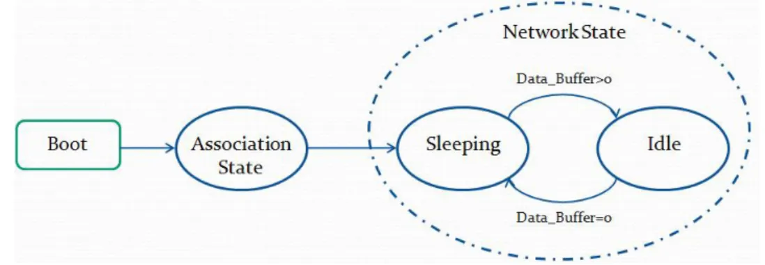
Association behavior synchronizes BP_Table Number of CPN and WSN. As shown in Figure 10, after WSN boots, the WSN device will set to Association State. The first thing to do is to listen beacon before joining the network. According to beacon information, WSN does time and BP_Table Number

15

synchronization, and replies an Association Request message to CPN.

The association behavior completes when WSN receives

Association Response replies from CPN. After that, WSN starts

to collect data. The device will change the Association State to

Network State.

 Network State

At the network state, the transceiver of WSN is in Sleeping

Mode most of the time. WSN will know when should receive

BP_Table and determine whether to turn on the transceiver for beacon or to stay in sleep. If there is no data frame in buffer, WSN will stay in the sleep mode and ignore the beacon. Otherwise, WSN will become Idle Mode and listen beacon. WSN transmits data according to the schedule timing in the received beacon. The change of state is also shown in Figure 10.

Figure 10: WSN state diagram

 Re-Synchronization

16

re-synchronization to maintain the time synchronization with CPN. By listening beacon, WSN adjusts the time offset and BP_Table Number.

3.2 Scenario

3.2.1 Single User Environment

The timing for CPN to send beacon is according to the BP_Table. Before CPN sends out the beacon, it will check current channel state is idle or busy by judging the Received Signal Strength Indicator (RSSI) of the air. If channel is idle, CPN will send the beacon. Else, it will cancel the transmission and wait for next transmission time.

The change of state is plotted in Figure 10 at Section 3.1.2. After WSN boots, the WSN’s state will set to Association State. When finishing association, the state will change to Network State. In Network State, WSN turns on/off its transceiver for receiving beacon or saving power according to BP_Table.

In single network, the transmission time of all the WSNs belonging to this network are scheduled by CPN. CPN broadcasts beacon to assign data slots for each WSN. According to the schedule in beacon, WSNs can transmit their data frames one by one without collision.

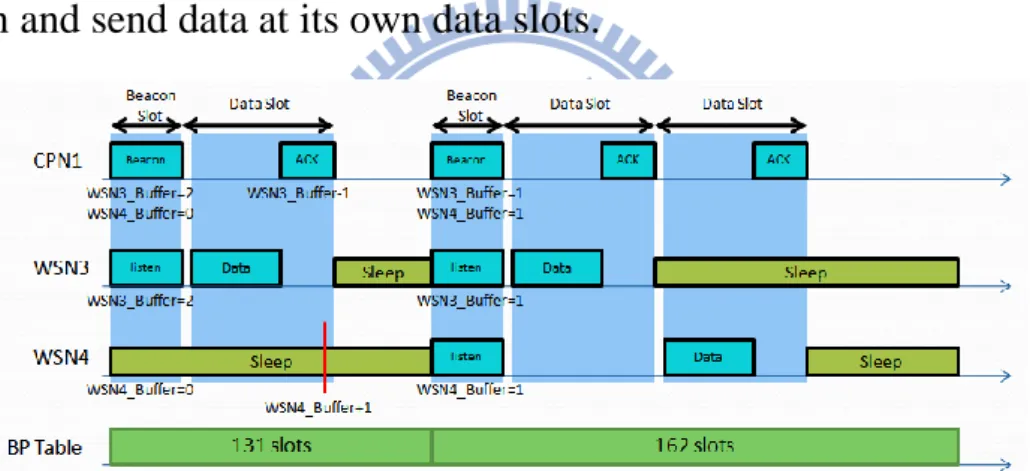
An example of single user environment timing diagram is shown in Figure 11. In the beginning, the number of data packet in WSN3’s buffer

17

is 2 and that in WSN4’s buffer is 0. According to the information of WSN’s buffers, CPN1 schedules one data slot for WSN3 and saves this schedule in beacon frame. When time reaches the scheduled transmission time, CPN1 broadcasts the beacon and announces the reserved data slots. Due to WSN3’s data buffer is not empty, WSN3 would receive the beacon and send data at its assigned data slots. For WSN4, because there is no data in its buffer, WSN4 would stay in the sleep mode and ignore the beacon. In the second round, due to there are data in the both WSNs’ buffer, CPN1 schedules two data slots for these two WSNs. When time reaches the scheduled transmission time, the WSNs would receive the beacon and send data at its own data slots.

Figure 11: Single user environment timing diagram

3.2.2 Multiple Users Environment

In multiple users environment, each network announces the channel occupied time by sending the beacon frame. Beacon frame contains the schedule information of transmission time and the schedule duration. When a CPN sends beacon successfully, the other CPNs which received this beacon will record the duration in their Network Allocation Vector so that they will cancel the beacon transmission in this NAV time period.

18

Therefore, the network’s WSNs can transmit data without interfering from other networks. Besides, due to the beacon interval is random in our design, the situation that a network always occupies channel might not happen, or we can say that the probability is low.

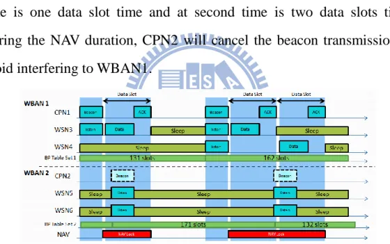
An example of multiple users environment timing diagram is depicted in Figure 12. The behavior of WBAN1 is the same as that shown in Figure 11. When CPN2 receives the beacon from CPN1, it records the reservation duration in its NAV. In this example, the NAV duration at first time is one data slot time and at second time is two data slots time. During the NAV duration, CPN2 will cancel the beacon transmission to avoid interfering to WBAN1.

Figure 12: Multiple users environment timing diagram

3.3 Simulation

3.3.1 Simulation Setup

 Network Density: place 5, 10, 20, 45, and 90 WBANs on 6m × 6m space, and each WBAN contains 1 CPN and 6 WSNs.

19

 Two moving speed scenarios: one is stationary (v= 0 m/s) and the other is moving (v= 1.4 m/s, based on walking speed). Moving path is

 Data Rate: each WSN generates one data packet per second.  The transceiver Tx and Rx mode power set to equal.

 Frame sizes are listed in Table 3. These frames are converted to slot time according to 3.6Mbps transmission rate: data frame is 12 slots, beacon frame is 11 slots and ACK frame approximates to 1 slot. (1 slot = 0.1ms)

Frame size Transmission time (ms)

Data frame 536 byte 1.2

Beacon frame 64 byte 1.14 (with 1 second preamble)

ACK frame 16 byte 0.035

Table 3: The size and transmission time of the frames

3.3.2 Beacon Period Table Based Protocol Simulation Result

The power consumption of WSN can be divided into Rx part and Tx part. Rx part is beacon receiving and Tx part is data transmission. The average power consumption is depicted in Figure 13. The total power consumption in the cases of stationary and moving are almost the same. This means that Beacon Period Table Based Protocol is good at adaptation for mobility and suitable for the characteristic of WBAN transmits in mobile.

20

The comparison chart of Rx part power consumption is shown in Figure 14. We can see the improvement of Rx part power consumption at high network density. Although the Rx part power consumption still increases as the network density, the slope is much smaller than that of 802.11 MAC protocol. By using the Beacon Period Table, WSNs can reduce the probability of idle listening so that the Rx part power consumption is a good improvement at high network density.

Figure 13: Average power consumptions per WSN per second

Figure 14: Beacon Period Table and 802.11 MAC protocol Rx power of WSN compare

21

Chapter 4 Implementation on TinyOS

In this chapter, we will introduce the implementation of the proposed protocol mentioned in Chapter 3.

4.1 TinyOS and Transmission Module Introduction

In this section, I will introduce the implementation environment. In WBAN, the sensor nodes have limited resources at memory and power, and also they need to handle complex transfer tasks, so the management system requires a miniature operating system. For this requirement, UC Berkeley researchers design an operating system, TinyOS [8], for wireless embedded sensor network. It features a component-based architecture which enables rapid innovation and implementation while minimizing code size as required by the memory constrains in the sensor network.

The transmission module has two main components, one is microprocessor MSP430 [9], and the other is transceiver chip CC1000 [10]. MSP430 microprocessor provided by TI is designed for low power and portable applications. And it also provides in-system programmable flash memory so that we can change the program code easily. CC1000 is a single-chip transceiver designed for low power and low voltage wireless applications. The main operating parameters of CC1000 can be programmed via an easy-to-interface serial bus, thus making CC1000 a flexible and easy to use transceiver. Besides, the transmission module also contains ECG sensor which is for ECG signals input and LEDs debugger which displays the module behaviors. The module is shown in

22

Figure 15.

Figure 15: The components of transmission module

4.2 MAC Architecture

4.2.1 Frame Type

There are four message types in our system. The Frame Type subfield is used to identify the frame type and shall be set to one of the values listed in Table 4.

Frame Type value Description

00 Beacon

01 Command

10 Data

11 ACK

Table 4: Values of the frame type subfield

a. Beacon frame field

23

Period Table Number with CPN. The BP Numer subfield contains current BP_Number of CPN. The NAV subfield is used to announce the channel occupy duration. The Schedule subfield contains the WSNs transmission time schedule.

b. Command frame field

Command frame is used to confirm the association behaviors. As the different Subframe Types, the message will be identified as Association_Request or Association_Response.

Frame Type Source Address Destination Address Subframe Type

c. Data frame field

WSNs transmit data by this format. Every time when WSN transmits a data frame, the Sequence Number subfield will increase by one to identify different data frames.

Frame Type Source Address Destination Address Sequence Number Data

d. ACK frame field

24

WSN that the data had been received successfully. The Sequence

Number value of ACK frame is the same as that of the received data

frame so that WSN can make sure which one data frame had been received.

Frame Type Source Address Destination Address Sequence Number

4.2.2 CPN Architecture

The main properties of CPN are providing network association, beacon sending and data receiving functions. The system architecture blocking diagram is shown in Figure 16. Afterward, we analyze the functions of each module to show the flow we proposed.

Figure 16: CPN architecture blocking diagram

a. Command Management

When the lower layer received frames, it will send Command Message to Command Management. Command Management responses

25

different messages based on the different kinds of received messages and sends Control Information to Beacon Generator module.

The detail blocking diagram of Command Management is presented in Figure 17. The main functions of this process are as following:

1. When receiving WSN Association Request message, the process will reply Association Response. Besides, it will send a WSN

Association message to inform Beacon Generator that a WSN has

connected.

2. When receiving Data Received message, the process will reply ACK frame and inform Beacon Generator that the node’s data had been received.

3. When receiving others CPN’s beacon frame, the process will check the NAV subfield and inform Beacon Generator the NAV locked duration.

26

b. Beacon Generator

According to the timing recorded in built-in Beacon Period Table, this process generates beacon frames. The contents of beacon frame are determined by the Control Information from Command Management.

The detail blocking diagram of Beacon Generator is presented in Figure 18. The main functions of this process are as following:

1. WSN Information Unit records the information of WSNs which connected to this CPN. The information includes the WSN’s ID, the number of data frames in WSN’s buffer and a timer counting the data collecting time. When the timer counts down to the end, the Number

of Data will increase by one.

2. When receiving the WSN Association message, Beacon Generator will create a WSN Information Unit to save the WSN’s information and start the timer to count the data collecting time of the WSN. 3. When receiving the Data Received message, the corresponding

WSN’s Number of Data will minus one.

4. According to Sequence Index, the process finds the corresponding time period in Beacon period Table and uses a timer to count it. When the timer counts down to the end, it will trigger Beacon Make to create a beacon frame.

5. The beacon frame contains:

 The BP Number subfield is from Sequence Index.

 The Schedule subfield is based on the Number of Data of WSN Information Units. Assign the data slots to the WSNs

27

which have data packets in the buffers.

 The NAV subfield is set to the time duration of the reserved time of Schedule subfield.

6. After Beacon Make creates a beacon frame, it will check the NAV

Timer. If NAV Timer is counting, Beacon Make will delete this

beacon frame. Else if the timer is idle, Beacon Make will send this beacon frame to Channel State Check module.

Figure 18: Beacon Generator blocking diagram

c. Channel State Check

When receiving beacon message, this process will check the RSSI value from Radio Control module. If the RSSI value is higher than a threshold, the process will cancel the beacon message transmission. Otherwise, it will transfer this beacon message to Radio Control module.

28

d. Radio Control

Radio Control controls CC1000 Tx/Rx modes switching and handles the input/output messages between MAC layer and CC1000 transceiver. The control behaviors are as following: In most of time, transceiver is in Rx mode. When receiving the packets needed to be transmitted, the process will switch transceiver to Tx mode. After the transceiver finished the transmission, it will return to Rx mode. Besides, Radio Control monitors the RSSI values of the air and provides the values to Channel State Check module.

4.2.3 WSN Architecture

The main properties of WSN are providing association, beacon receiving, data transmission and radio power saving functions. The system architecture blocking diagram is shown in Figure 19. Afterward, we analyze the functions of each module to show the flow we proposed.

29

a. Command Management

When the lower layer received frames, it will send Command Message to Command Management. Command Management responses different messages based on different kinds of received messages and sends Control Information to Beacon Generator module and Data

Control module.

The detail blocking diagram of Command Management is presented in Figure 20. The main functions of this process are as following:

1. When receiving Association Response message, the process will save the CPN’s ID. This behavior means WSN has joined in the network successfully.

2. When receiving ACK message or NOACK message, the process will transfer the message to Data Control module as the data transmission reaction.

3. When receiving Beacon message, the process will set the Sequence

Index of BP_Table according to the BP Number subfield of the

beacon frame and set the Schedule Timer according to the Schedule subfield. When Schedule Timer counts down to the end, it will trigger a Data Transmit message to Data Control module.

b. Beacon Management

Beacon Management determines when the transceiver should receive beacon frame. According to Sequence Index, the process finds the

30

corresponding time period in Beacon period Table and uses a timer to count it. When the timer counts down to the end, it will trigger a Beacon

Receive message to Radio Control module. The detail blocking diagram

of Beacon Management is also shown in Figure 20.

Figure 20: Command Management and Beacon Management blocking diagram

c. Data Control

According to command message from Command Management, this process controls the data transmission or retransmission. The main functions of this process are as following:

1. The Data Buffer uses FIFO (first in, first out) concept to output the data. When receiving Data Transmit message, Data Control will request Data buffer for a data packet which is called Current Data and transfer this data packet to Radio Control.

2. When receiving ACK message which means CPN received data successfully, the process will delete Current Data and request for a

31

new data packet when next time receiving Data Transmit message. 3. If the reaction message is NOACK which means CPN didn’t reply

ACK frame, the process will remain the Current Data and still transmit this data packet when next time receiving Data Transmit message.

The Schematic diagram of Data Buffer and Data Control is shown in Figure 21.

Figure 21: Schematic diagram of Data Buffer and Data Control

d. Radio Control

The Radio Control of WSN is basically like that of CPN. In addition to the Tx/Rx modes, we add Sleep Mode for power saving purpose and use Control Unit to management the mode change. The blocking diagram of Control Unit is shown in Figure 22. The Control Unit is made up of two timers, Beacon Receive Timer and ACK Response Timer.

1. When receiving Beacon Receive message, the process will switch the transceiver to Rx mode and turn on Beacon Receive Timer simultaneously. When the timer counts down finished, the process will switch the transceiver to Sleep mode.

32

2. When receiving Data Transmit message, the process will switch the transceiver to Tx mode and turn on ACK Response Timer. When the timer counts down to the end, the process will switch the transceiver to Sleep mode, and if the WSN doesn’t receive the correct ACK frame from CPN, the process will send NOACK message to Command Management.

Figure 22: Control Unit blocking diagram

4.3 Power Consumption Analysis

4.3.1 Environment Setting

In our implementation scenario, we use WBAN to transmit Electrocardiography (ECG) data. The device settings are as following:  The sampling rate is 25Hz and 1 byte per sampling.

 The data packet size set to 100 bytes.

 The transmission rate of transceiver CC1000 is 9.6 Kbps.

Therefore, to achieve real-time transmission, each WSN shall send one data packet per 4000ms.

33

We prepared two WBANs to test the network merging effect. Each WBAN is including one CPN and two WSNs as shown in Figure 23. WSNs sense the ECG data and transmit it to CPN. After receiving the ECG data, CPN pass it to computer and display on the java platform which is shown in Figure 24.

34

Figure 24: ECG data on the java platform

4.3.2 Power Measurement

In order to calculate the power consumption of WSN, we can use ZXCT1010 [11] chip which is a high side current sense monitor. We use this chip to convert the device’s current to voltage and monitor the voltage by Oscilloscope. The circuit of ZXCT1010 with the transmission module is shown is Figure 25.

Figure 25: The circuit of ZXCT1010 with the transmission module

From the data sheet, we set: Rsense = 0.1 Ω

35

Vsense = Vin – Vload

Vout = 0.01*Vsense*Rout

Iload =

=

The voltage Vout of WSN in one cycle shown on Oscilloscope is

presented in Figure 26.

Figure 26: The current consumption of WSN in one cycle

We convert Vout to Iload according to the above formula. A cycle of

WSN is including Beacon receiving, data sending, ACK receiving and sleep mode. The current and time consumption of each part are shown in Table 5.

36

We can calculate the average power consumption of WSN according to the following parts:

1. Beacon receiving and Data transmission success

WSN transmits one data frame per 4000ms in general. 38.2mA * ( ) + 24.7mA * ( ) + 2.2mA * ( ) = 8.78

2. Idle beacon receiving

When the CPN is in a NAV locked state, the WSNs will still wake up and listen for beacon. In our experimentation, the probability of idle beacon receiving is 43%.

38.2mA * (

) * 43% = 1.15

3. Data transmission failure

If WSN doesn’t receive ACK after sending data frame, this transmission will be judged as a failure. In our experimentation, the probability of data transmission failure is 3%. {38.2mA * ( ) + 24.7mA * ( ) + 2.2mA * ( )} * 3% = 0.26

 Average power consumption is about 10.2

In this experimentation, the probability of idle beacon receiving is up to 43%. It’s because the transmission rate of transceiver is low so that the time of channel occupied for one network is too long. The WSNs can’t transmit their data in the NAV duration. Therefore, they will wake up to listen for beacon every time until they transmit all the data in the buffers.

37

This behavior increases the probability of idle beacon receiving.

The probability of data transmission failure is 3%. If the networks are still sending their data packet at the moment that the networks encounter, the transmission failure will happen. However, after CPNs receive the beacon of each other, the transmission failure seldom happens.

38

Chapter 5 Conclusion

In this thesis, we present a TDMA based network merging method for single channel WBAN system. At first, we analyze and simulate the IEEE802.11 MAC protocol. It seems that the protocol has some issues on power consumption in high network density scenario. Therefore, we propose the network merging method. By using schedule function of CPN and Beacon Period Table, WSNs can reduce the idle time and the probability of transmission collision so that they can save most power. This method has been proved to be more power efficiency compared to IEEE802.11 in high network density scenario. Finally, we implement this system on TinyOS and test the network merging effect and power consumption of the actual operation on the transmission module.

39

REFERENCES

[1] Sana Ullah, Bin Shen, S.M. Riazul Islam, Pervez Khan, Shahnaz Saleem and Kyung Sup Kwak, "A study of MAC protocols for WBANs," Sensors, 28 December 2009.

[2] ShihHeng Cheng, MeiLing Liu, ChingYao Huang, "Radar Based Network Merging for Low Power Mobile Wireless Body Area Network," 4th International

Symposium on Medical Information and Communication Technology, Taipei, Mar,

22-25, 2010.

[3] Bluetooth SIG Inc., "Specification of the Bluetooth system: Core," Available:

https://www.bluetooth.org/

[4] LAN-MAN Standards Committee of the IEEE Computer Society, "IEEE 802.15.4 2003 standard, Wireless Medium Access Control (MAC) and Physical Layer (PHY) Specifications for Low-Rate Wireless Personal Area Networks (LR-WPANs)," 12 May 2003.

[5] Mattbew S. Gast, "802.11 Wireless Networks: the Definitive Guide," Sebastopol,

CA: O’Reilly, 2002.

[6] 黃能富。"區域網路與高速網路"，維科出版社，1998。

[7] Hsieh, Kun-Lung, "A prompt formation algorithm for IEEE 802.15.3 Ad Hoc networks," NTU Institutional Repository, 2004.

[8] TinyOS community forum. Available at: http://www.tinyos.net/

[9] Texas Instruments, "MSP430x11x Mixed Signal Microcontrollers," 2004.

[10] Texas Instruments, "SmartRF CC1000 Preliminary Datasheet (rev. 2.1)," 19 April 2002.

[11] ZETEX Semiconductors, "Enhanced high-side current monitor, ZXCT1010," July 2007.