國 立 交 通 大 學
土 木 工 程 學 系
博 士 論 文
利用多衛星測高資料改善全球重力異常模型以及淺海
區重力異常
Improved Determinations of Global Gravity Anomaly
Model and Shallow-Water Gravity Anomalies from
Multi-Satellite Altimetry
研究生:徐欣瑩
指導教授:黃金維
中華民國九十六年六月
利用多衛星測高資料改善全球海洋重力異常模型以及淺海
區重力異常
研究生:徐欣瑩 指導教授:黃金維
國立交通大學土木工程研究所
摘要
本論文的內容主要是致力於改善全球海洋重力異常模型以及淺海區重力異 常。本研究結合 Seasat, Geosat/GM, Geosat/ERM, ERS-1/35day, ERS-1/GM, ERS-2, 以及 T/P 等七種衛星測高任務資料來推求全球海洋重力異常模型以及 全球平均海水面模型,以 2'X 2'的解析度涵蓋全球南緯 80 度到北緯 80 度的 區域範圍。全球平均海水面模型透過與 T/P 以及 ERS-1 的平均海水面模型進行比 較,可分別得出 5.0 公分以及 3.1 公分的均方根值。在全球選擇出十二個區域, 進行船測重力異常與全球重力異常模型之比較,得出其差值之均方根值最大為 13.4mgals,最小為 3.0mgals。 為改善衛星測高的資料品質,本研究從資料偵錯以及資料型態兩方面著手, 採用一種非線性的濾波函數對沿軌跡的測高資料進行粗差偵測,以及採用海水面 高度值一次差作為資料型態,研究成果顯示可以得出較佳的重力異常。本研究選 擇東海海域以及台灣海峽作為改善淺海區重力異常的研究區域,在此兩區域比較 兩個不同的全球海洋測高重力異常模型,將兩模型的差異值進行分析討論,可以 得出重力異常的差異與海潮模式的選擇、海水面高度值的中誤差以及海深有其相 關性。 為改善淺海區重力異常,本研究採用不同的資料型態搭配計算方法產生三種 推求重力異常的方法進行測試:第一種方法是採用最小二乘預估法,資料型態採 用海水面高度值一次差以及海水面高度值的梯度值;第二種方法是採用沿軌跡的 垂線偏差值作為資料型態以最小二乘預估進行計算重力異常;第三種方法是採用最小二乘預估將沿軌跡垂線偏差組成網格,再以 inverse Vening Meinesz 公式 進行計算。以上三種方法在台灣海峽進行淺海區重力異常計算,並與船測重力進 行比較,分別得出其差值的均方根為 9.06,10.26,10.44 以及 10.73 mgals;在東 海區域分別得到的結果是 9.59,9.77,13.10,11.86 mgals。由此可知採用海水面 高度值一次差以及海水面高梯度值作為測高資料型態可以得出較佳的重力異常 成果。對於陸地沿岸的淺海區重力異常推求,若加入沿岸陸地重力資料,可以明 顯改善淺海區的重力異常,本研究在台灣海峽沿岸進行測試,得出差值的均方根 為 8.22mgals。
Improved Determinations of Global Gravity Anomaly
Model and Shallow-Water Gravity Anomalies from
Multi-Satellite Altimetry
Phd Student: Hsin-Ying Hsu Advisor: Cheinway Hwang
Department of Civil Engineering
National Chiao Tung University
ABSTRACT
This dissertation is aimed at improved determination of global and shallow water gravity anomalies. Global mean sea surface heights (SSHs) and gravity anomalies on a 2´×2´ grid were determined from Seasat, Geosat (ERM and GM), ERS-1 (1.5-year mean of 35-day, and GM), TOPEX/POSEIDON (T/P) (5.6-year mean) and ERS-2 (2-year mean) altimeter data over the region 0°-360° longitude and –80°-80° latitude. The comparison of the global mean sea surface height (MSSH) with the T/P and the ERS-1 MSSH result in overall RMS differences of 5.0 and 3.1 cm in SSH, respectively, and 7.1 and 3.2 µrad in SSH gradient, respectively. The RMS differences between the predicted and shipborne gravity anomalies range from 3.0 to 13.4 mgals in 12 areas of the world oceans.
To improve the altimeter data quality, a nonlinear filter with outlier rejection is applied to along-track data, and differenced height is found to be most sensitive to this method. The differences of two global satellite altimeter-derived gravity anomaly grids over the East China Sea (ECS) and the Taiwan Strait (TS) are investigated and
the causes of the differences are discussed. Difference of gravity anomaly is correlated with tide model error, standard deviation of sea surface heights (SSHs) and ocean depth.
To improve the shallow water gravity anomalies, three methods of gravity anomaly derivation from altimetry were compared near Taiwan and East China Sea: (1) compute gravity anomalies by LSC using along-track, differenced geoidal heights and height slopes, (2) compute gravity anomalies by least-squares collocation (LSC) using altimeter-derived along-track deflections of vertical (DOV), and (3) grid along-track deflections of vertical by LSC and then compute gravity anomalies by the inverse Vening Meinesz formula. For the three methods, the RMS differences between altimetry-derived gravity anomalies and shipborne gravity anomalies are 9.06 (differenced height) and 9.59, 10.26 (height slope) and 9.77, 10.44 and 13.10, 10.73 and 11.86 mgals, in Taiwan Strait and East China Sea respectively. Two new SSH-derived observations of altimetry (differenced height and height slope) were presented for gravity derivation and use of differenced heights in LSC produces the best result. Use of land gravity data in the vicinity of coasts was implemented near Taiwan and this enhances the accuracy of altimeter-derived gravity anomalies at a RMS difference of 8.22 mgals.
CONTENTS
ABSTRACT (in Chinese) I ABSTRACT Ⅲ CONTENTS Ⅴ LIST OF FIGURES Ⅷ LIST OF TABLES ⅩI
CHAPTER 1 INTRODUCTION 1
1.1 Development of Satellite Altimetry……….1
1.1.1 Past Satellite Altimetry Missions…..……….1
1.1.2 Current and Future Satellite Altimetry Missions……… 5
1.2 Objectives and Outline……….……….13
CHAPTER 2 MARINE GRAVITY ANOMALIES FROM SATELLITE ALTIMETRY 15
2.1 Introduction………...15
2.2 Marine Gravity Field from Altimetry………15
2.2.1 Overview………..15
2.2.2 Remove-restore Technique……….. 17
2.2.3 Altimeter Data Types……….18
2.3 Methods of Marine Gravity Anomalies from Altimetry………20
2.3.1 Method 1: Least Squares Collocation………..………20
2.3.2 Method 2: Inverse Venning Meinesz Formula……….24
2.3.3 Method 3: Fourier Transform with Deflection of Vertical…….…..25
2.4 Radar Altimeter Data………29
2.4.1 Altimetry Data and Observations………29
2.4.2 Time-averaging of SSH………...32
2.5 Multi-Satellite Altimeter Data Processing………. 33
2.5.1 Altimetry Data Base………33
2.5.2 Averaging SSH to Reduce Variability and Noise……….35
2.5.3 Choice of Ocean Tide Model……….. 37
CHAPTER 3 GLOBAL MODELS OF MEAN SEA SURFACE AND GRAVITY ANOMALY 41
3.1 Introduction……….. 41
3.2 Forming North and East Components of DOV……….42
3.2.1 Computing Along-track DOV………. 42
3.2.2 Removing Outliers and Gridding DOV………..…….44
3.3 Conversions from DOV to MSSH and Gravity Anomaly………..47
3.4 Computation and Analysis of Global MSSH Model………..49
3.5 Computation and Analysis of Global Gravity Anomaly Model……….55
CHAPTER 4 DATA PROCESSING AND METHODS OF GRAVITY DERIVATION OVER SHALLOW-WATERS 58
4.1 Introduction………..58
4.2 Data Processing:Outlier Detection and Filtering……….…………..59
4.3 Results of Tests………..…...……….……….70
CHAPTER 5 GRAVITY ANOMALY OVER EAST CHINA SEA AND TAIWAN STRAIT: CASE STUDY AND ANALYSIS 74
5.1 Introduction………...74
5.2 Comparison of Two Global Gravity Anomaly Grids over ECS and TS……77
5.3 Coastal Land and Sea Data for Accuracy Enhancement………...84
5.4 Outlier Distribution……...………85
5.5 Case Studies………..88
5.5.1 The East China Sea………..88
5.5.2 The Taiwan Strait…..………...93
CHAPTER 6 CONCLUSIONS AND RECOMMENDATIONS 100
6.1 Conclusions……….. 100
6.2 Recommendations………102
LIST OF FIGURES
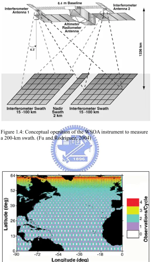
Figure 1.1: The ground tracks of Geosat/ERM around Taiwan………...……….6 Figure 1.2: The ground tracks of EnviSat around Taiwan……….8 Figure 1.3: The ground tracks of Jason-1 around Taiwan………...10 Figure 1.4: Conceptual operation of the WSOA instrument to measure a 200-km
swath. (Fu and Rodriguez, 2004)………12
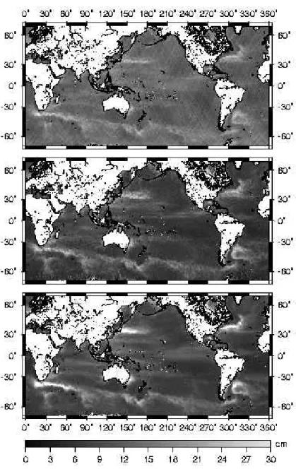
Figure 1.5: Coverage map for WSOA showing the number of observations per 10-day
cycle for a 200-km swath. (Fu and Rodriguez, 2004)………..12
Figure 2.1: Geometry for the inverse Vening-Meinesz formula………..25 Figure 2.2: Schematic illustration of the measurement principle. (from
http://www.aviso.oceanobs.com/html/alti/principe_uk.html)…...32
Figure 2.3: Estimated standard deviations of point SSH of Geosat/ERM (top), ERS-1
(center) and TOPEX/POSEIDON (bottom)……….38
Figure 3.1: Quasi time-independent sea surface topography from Levitus et al. (1997),
contour interval is 10 cm………..44
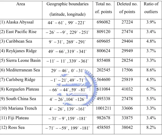
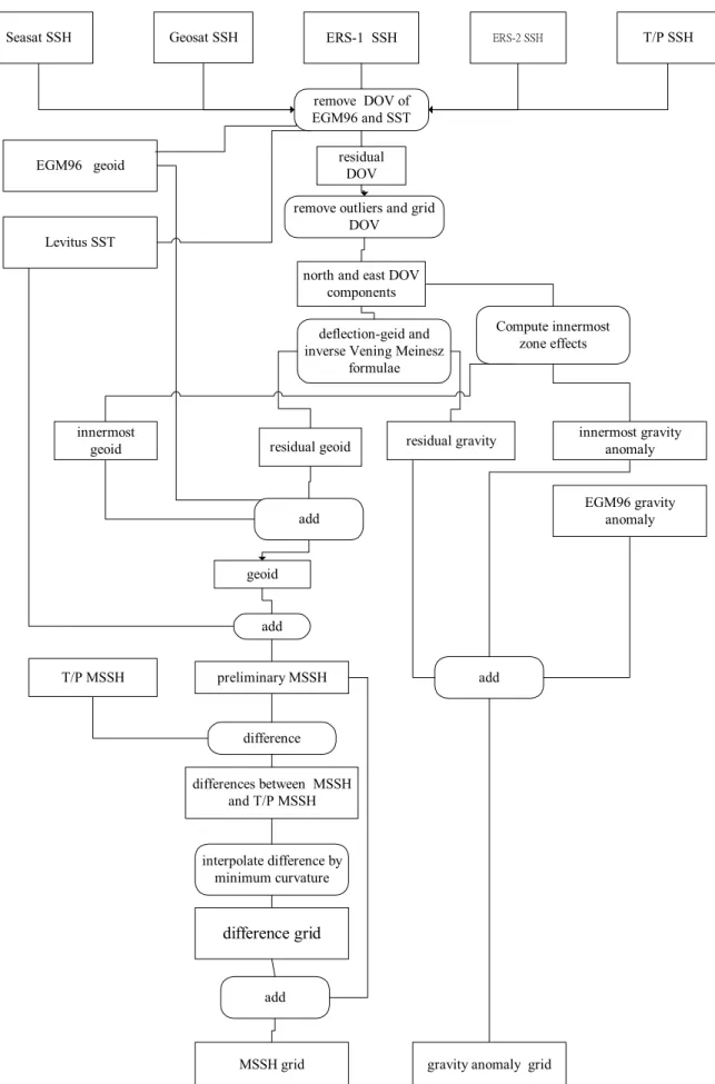
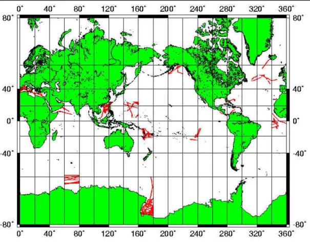
Figure 3.2: Flowchart for computing global MSSH and gravity anomaly grids…….52 Figure 3.3: Difference between NCTU01 and T/P mean sea surface heights……….53 Figure 3.4: Distributions of shipborne gravity anomalies in the 12 areas where the
NCTU01 gravity anomaly grid is evaluated………56
Figure 4.1: Contours of slected depths around Taiwan, unit is meter……….60 Figure 4.2: The ground track of pass d64 of Geosat/ERM ………62 Figure 4.3: Raw data points (red) and outliers (green) detected with a 28-km window
for pass d64 of Geosat/ERM………63
Figure 4.4: The ground track of pass a27 of Geosat/GM………63 Figure 4.5: Raw data points (blue) and filtered and outlier-free points (red) using a
14-km window for pass a27 of Geosat/gm……….…..64
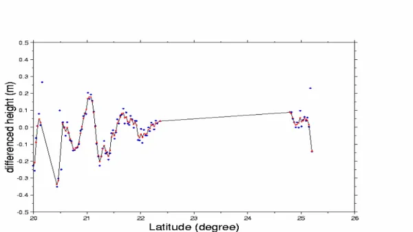
Figure 4.6: The ground tracks of Geosat/GM d0222 and a3083……….64 Figure 4.7: Differenced heights for passes d0222 and a3083 of Geosat/gm, crosses
represent outliers………..65
Figure 4.8: Ascending and descending passes of Geosat/ERM for outlier detection..66 Figure 4.9: Results with a 28-km window size. Outliers are not connected by the
lines. ………67
Figure 4.10: Ascending and descending passes of Geosat/GM for outlier detection..68 Figure 4.11: Results with a 18-km window size. Outliers are not connected by the
lines………..69
Figure 4.12: Distribution of shipborne gravity data in Taiwan Strait area…………..72 Figure 4.13: Distribution of shipborne gravity data in the East China Sea………….72
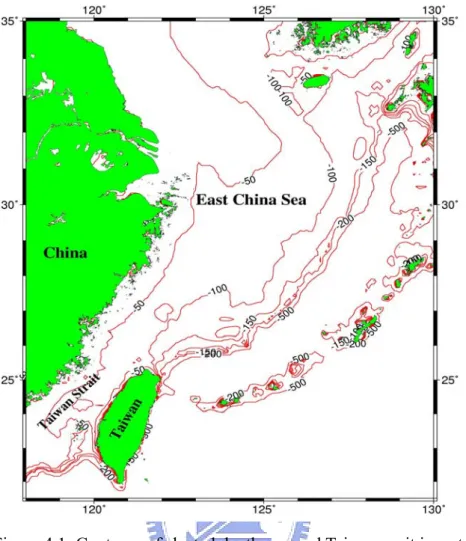
Figure 5.1: Bathymetry (dashed lines) in the East China Sea and Taiwan Strait. Lines
represent shipborne gravity data for comparison with altimeter-derived gravity
anomalies………..76
Figure 5.2: Differences between the SS02 and KMS02 global gravity anomaly
grids………..78
Figure 5.3: Standard deviations of sea surface heights from the Geosat/ERM,
ERS-1/35 day and ERS-2/35 day repeat missions………. .79
Figure 5.4: Differences between the NAO and CSR4.0 tidal heights at a selected
epoch………81
difference and depth, along Track 1……….82
Figure 5.5b: Time series of normalized standard deviation of ERS-1 SSH, tide height
difference and depth, along Track 2……….83
Figure 5.6: Distribution of altimeter data outliers in East China Sea………..86 Figure 5.7: Distribution of altimeter data outliers in Taiwan Strait. ………...87 Figure 5.8: Gravity anomalies along Cruises c1217 and dmm07 in the East China
Sea………91
Figure 5.9: Time series of normalized difference of gravity anomaly, standard error of
ERS-1 SSH, tide model difference and depth, along Cruise dmm07………...92
Figure 5.10: Time series of normalized difference of gravity anomaly, standard error
of ERS-1 SSH, tide model difference and depth, along Cruise c1217………...93
Figure 5.11: Distribution of land gravity data and altimeter data around Taiwan…...95 Figure 5.12: Gravity anomalies along Track 1 and Track 2 in the Taiwan Strait……96 Figure 5.13: Time series of normalized difference of gravity anomaly, standard error
of ERS-1 SSH, tide model difference and depth, along Track 1……….98
Figure 5.14: Time series of normalized difference of gravity anomaly, standard error
LIST OF TABLES
Table 2.1: Specifications for satellite missions………...………29 Table 2.2: Satellite altimeter missions and data used for the global computation…...34 Table 2.3: Statistics of SSHs from seven satellite altimeter missions……….37 Table 2.4:RMS collinear differences (in cm) of T/P (Matsumoto et al. 2000) and
corresponding error (in µrad) in along-track DOV of Geosat/GM using different tide models………..39
Table 2.5: RMS differences (in mgals) between shipborne and altimeter-derived
gravity anomalies with different tide models………...40
Table 3.1: Test areas and ratios of removed outliers………46 Table 3.2: RMS differences (in cm) between global sea surface models and T/P and
ERS-1 MSSH ………..53
Table 3.3: RMS differences in along-track sea surface height gradients (in µrad)
derived from global sea surface models and from T/P and ERS-1 MSSH…………..54
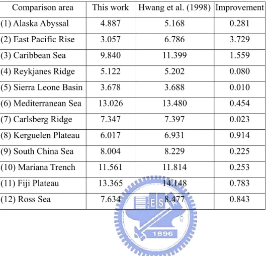
Table 3.4: RMS differences (in mgal) between predicted and shipborne gravity
anomalies in 12 areas………...57
Table 4.1: RMS differences (in mgals) between predicted and shipborne gravity
anomalies using different filter parameters over the Taiwan Strait……….71
Table 4.2: RMS differences (in mgals) between predicted and shipborne gravity
anomalies using different filter parameters over the East China Sea………..71
Table 4.3: Statistics of differences (in mgals) between altimeter-derived and
shipborne gravity anomalies……….73
Table 4.4: Statistics of differences (in mgals) between altimeter-derived and
shipborne gravity anomalies in the East China Sea……… 73
anomaly grids over the area 118°−130°E,22°−35°N………77
Table 5.2: Summary of outliers rejection in the East China Sea (119/131/25/35)….87
Table 5.3: Summary of outliers rejection around Taiwan (117/125/20/28)……….88
Table 5.4: Statistics of differences (in mgals) between altimeter-derived and
shipborne gravity anomalies in East China Sea………..90
Table 5.5: Statistics of differences (in mgals) between altimeter-derived gravity and two tracks of shipborne gravity anomalies in Taiwan Strait………90
Table 5.6: Statistics of difference (in mgals) between altimeter-derived and shipborne gravity anomalies in the Taiwan Strait………....90
CHAPTER 1
INTRODUCTION
1.1 Development of Satellite Altimetry
1.1.1 Past Satellite Altimetry Missions
From 1980s, with the advanced development of computer science and space technology, the study of the earth science itself has changed as we better understand everything from the macroscopic aspect to microcosmic dimension. Over the past few decades satellite altimetry has developed into a new way to study the earth. The basic concept is very simple. The satellite is used as a moving platform, with a sensor to receive the return signals after reflection at the earth’s surface. Through data processing and analysis, we can study the problems of geodesy, geophysics and oceanography.
Satellite altimetry has only been around for 30 years, but even though it is still a very young science, the results of its research explain geoid and gravity anomaly better than ever before. Its history demonstrates huge potential in improving the study of the global gravity field, and studying the oceans currents and surface. Satellite altimetry shows the structure of the bottom of the ocean from a viewpoint that has never before been possible. Because of its characteristics: worldwide range, high accuracy, rapid and periodic, satellite altimetry can help us explore all kinds of phenomena in earth sciences. Therefore we can take the study of the earth to another level providing extensive information about the earth.
The first satellite launched exclusively for altimeter research was called Skylab (Seeber, 1993). Skylab was launched on 9, April 1975, and was the first satellite of its kind specifically designed to research the physical attributes of the ocean by satellite. The experiment didn’t yield many results but was a good foundation for future missions such as Geos-3 through the National Aeronautics Space Administration (NASA).
Skylab weighed 345.9kg, orbit altitude is 840km, with an incline angle is 115°. Its lifespan was 3.5 years, repeating its orbital cycle every 23 days with an altimeter accuracy of about 25~50cm. The satellite was designed to provide useful parameters of oceanography and geodynamics for over 3 years enhancing our capability to earth gravity field, the shape and the size of geoid, deep ocean tide, ocean current structure, the crust structure and rigid geodynamics etc. Geos-3 was successfully launched into regular orbit, which is a model mission for future satellites to be launched.
On June28, 1978, Seasat (Sea Satellite) altimeter was launched with a new remote sensing technique. This new method of researching ocean science began a new era of ocean exploration. The satellite has an altitude of 800km, at an incline angle of 108˚. This satellite is expected to function for 106 days, the first repeat cycle is 3 days, and the post repeat cycle is 17 days, with an accuracy of about 20~30cm. Seasat was launched to provide a remote sensing technique that could measure the whole earth very precisely while measuring the temperature, current and tides of the ocean simultaneously. In spite of the fact that Seasat worked perfectly in orbit for almost 3 months, the electronics of altimeter malfunctioned and it stopped working, but it still provided a lot of statistics about the ocean even after it malfunction. Through satellite altimetry we have advanced so much in our knowledge of ocean geoid, sea surface terrain, marine gravity, the seafloor, geodynamics and oceanography that there is no
In order to efficiently develop accurate measurements, correctly measure earths gravity field, understand the shape of the geoid, and make up for the weakness of Seasat for its short life span that limits the amount of time to collect information, the American Navy launched the Geosat (Geodetic Satellite) satellite altimeter on March 12, 1985. Its primary mission was to precisely measure all gravity fields throughout the entire world. Geosat’s average orbit altitude is 800km, with an inclination angle of 108 degrees. Geosat will repeat its cycle every 17 days throughout its functional lifespan of more than 4 years. Geosat is accurate within about 10~ 20cm. It took 18 months from its launch date in March 1985, through 30 Sept 1896 for the Geosat satellite to complete its mission of tracking the entire earth in 4km intervals. The tracks that were flown while measuring the worlds great oceans combined would measure 200 million km, and the project collected 270 million measurements.
Geosat orbit repeats every 17 days in precisely the frozen orbit, this is called an Exact Repeat Mission (ERM). Statistics from the Geosat, satellite altimeter data are used to gather information about earth gravity field, sea mountain, oceanic trench, ocean floor over a very wide area. This project was a huge accomplishment and the first of its kind. The information gathered in satellite altimetry has been tested and has proved to be very accurate in measuring the global geoid, gravity anomaly, gravity disturbance, establish a higher degree gravity model, seafloor, geological structure, solid geophysics, oceanography, ocean tide, and ocean current. There are many possibilities for the uses of satellite altimetry in the future.
The European Space Agency (ESA) after ten years of preparation launched the first European Remote-Sensing Satellite (ERS-1) on July 17, 1991, ERS-1’s average altitude is 785km, the incline angle is 98.5˚, and orbits the earth every 100 minutes throughout its 3 year life. Its main mission is to study the Earth’s atmosphere and its
ocean. During its first 3 months in orbit ERS-1 will cover the whole earth every three days. ERS-1 has the ability to adjust its orbital altitude and cycle. After the first three months the satellite switched to normal orbital cycles every 35 days. At the end of its mission the satellite repeated every 168 days.
ERS-1 measures ocean waves, wind field and its change, ocean circulations, global sea level change, and provides satellite images of both land and ocean, sea surface topography, sea surface temperature, and sea surface vapor and may other things. ERS-2, the follow-on of ERS-1, was used together with it from April 1995 to June 1996, their identical orbits (35 days) have a one-day shift.
In order to be more accurate in measuring the surface of the ocean, and in researching ocean circulation and ocean tide, NASA and CNES jointly launch Topex/Poseidon (T/P) on Aug 10, 1992, a satellite mission with the objective of "observing and understanding the ocean circulation". Its altitude in orbit is about 1336 km, with an inclination angle of 66˚. Topex/Poseidon is capable of covering 90% of both the earth and ocean, it has a repeat cycle of 10 days and collects statistics on the whole earth 35 times each year.
The main purpose of the Topex/Poseidon mission is monitoring global sea surface height, determining the ocean currents and measuring the effect of these currents on the surrounding areas. This information provide statistics about the parameter of the ocean for the whole world. So far T/P has the best performance on the accuracy of precision orbit determination in all altimetry mission.
Because of the significant meaning of altimeter data in geodesy, oceanography and geophysics, the ERS-1-follow-on, ERS-2 were launched in April 1994. Geosat
before Jason-1, which was launched on December 7, 1992. Lots of advancement have been made in altimeter technology that have advanced all areas of researching the ocean. The satellites have collected enormous amounts of data that still need to be researched.
1.1.2 Current and Future Satellite Altimetry Missions
(1) GEOSAT Follow-On 1 (GFO-1 )
The GEOSAT Follow-On 1 (GFO-1) program is the U.S. Navy's plan to develop an workable series of radar altimeter satellites to continuously monitor the ocean observations from the GEOSAT Exact Repeat Mission (ERM) orbit (800 km altitude, 108˚ inclination, 0.001 eccentricity, and, 100 min period). GFO-1 is the follow-on to the highly successful GEOSAT and was launched in February 1998. On 29 November 2000, the U.S. Navy declared the satellite as operational.
The first 17-day Cycle after the U.S. Navy began using it is numbered 000 and is used as a reference for the succeeding cycles. After the reference cycle, the first 17-day cycle which started on December 16, 2000 (Julian day 352) is the beginning of the first evaluation cycle, Cycle 001, which ended on 2 January 2001 (Julian day 2001 002). Each following 17 day cycle is consecutively numbered. This 17-day Exact Repeat Orbit (ERO) retraces the same ERM ground track to +/-1 km. As with the original GEOSAT ERM, the data will be available for ocean science through NOAA/NOS and NOAA/NESDIS.
The 5-year GEOSAT mission with its extensive data validation program confirmed the ability of the radar altimeter to measure the dynamic topography of the western boundary currents such as the Gulf Stream, as well as their associated rings
and eddies, to provide sea surface height data for assimilation into numerical models, and to map the progression of El Nino in the equatorial Pacific. Figure 1.1 is the ground tracks of Geosat/ERM (the same as GFO-1) around Taiwan.
Figure 1.1: The ground tracks of Geosat/ERM around Taiwan.
(2) Environmental Satellite (EnviSat)
The main objective of the Envisat program is to provide Europe with an improved capability for the remote sensing observation of Earth from space. The goal is to increase the capacity of participating states to become involved in the studying and monitoring of the Earth and its environment.
Its main goals are: to provide for continuity and stability of the observations started with the ERS satellites, including those obtained from radar-based observations; to enhance the ERS mission, specifically the ocean and ice mission; to
that effect the environment; to make a significant contribution to environmental studies, notably in atmospheric chemistry and ocean studies (including marine biology).
These are together with two secondary objectives: to allow more effective monitoring and management of the Earth's resources; to better understand the processes of solid Earth.
The mission intends to continue and improve the measurements began by ERS-1 and ERS-2, it will take into account the requirements related to the global study and monitoring of the environment. The mission is an essential part in providing long-term continuous data sets that are crucial for addressing environmental and climatological issues. It will at the same time push for a gradual change in the use of remote sensing data from experimental to operational exploitation.
Envisat, as an undertaking of ESA member states plus Canada, constitutes a major contribution to the international effort of space agencies worldwide to provide the data and information required to further the understanding, modeling, and prediction of environmental and climatic changes. Figure 1.2 shows the ground tracks of ERS-2 (EnviSat) around Taiwan.
Figure 1.2: The ground tracks of EnviSat around Taiwan.
(3) Jason-1
JASON-1 is a follow-on mission to the highly successful TOPEX/POSEIDON (T/P) mission. It was developed by the French Space Agency, the Centre National d’Etudes Spatiales (CNES) and the United States National Aeronautics and Space Administration (NASA), for the study of global circulation from space. The mission uses the technique of satellite altimetry to make precise and accurate observations of sea level for several years. Jason-1 continues Topex/Poseidon's observations of ocean surface topography to monitor world ocean circulation. It studies interactions of the oceans and atmosphere, improves climate predictions and observes events like El Nino.
The main goal of this mission is to measure the sea surface topography with the same quality as T/P. The mission will provide a large continuous time series of highly-accurate measurements of the ocean topography from which scientists can determine the general circulation of the ocean, and understand its role in the Earth’s
climate. In addition to the primary JASON-1 IGDR and GDR data products provided with a 5 and 30 day latency, respectively, JASON-1 also supports the preparation of operational ocean services by providing a non-validated near-real-time (3 hour latency) JASON-1 data product, the Operational Sensor Data Record (OSDR). JASON-1 is the first in a twenty-year series of satellites to take over from T/P, marking the start of operational satellite altimetry.
The global oceans are Earth's main storehouse of solar energy. Jason-1's measurements of sea-surface height reveal where this heat is stored, how it moves around Earth by ocean currents, and how these movements affect the weather and climate. Jason-1 is designed to directly measure climate change through very precise millimeter-per-year measurements of global sea-level changes.
Weighing 500 kilograms (about 1,100 pounds), Jason-1 is one-fifth the size of Topex/Poseidon. Jason-1 flew together with Topex/Poseidon until Topex/Posiedon stopped working, this doubled the scientific data measured. Figure 1.3 shows the ground tracks of Jason-1 around Taiwan.
Figure 1.3: The ground tracks of Jason-1 around Taiwan.
(4) Jason-2: WSOA (Wide-Swath Ocean Altimeter)
A pulse-limited radar altimeter such as T/P provides profiles of sea-surface height along the satellite's ground tracks with a spatial resolution of 6-7 km. Such profiles may be used to obtain information about ocean surface currents and the marine gravity field. However, this measurement is basically one-dimensional and does not provide a complete picture of the vector field of ocean currents and gravity anomalies. In order to map the sea-surface height in two dimensions with comparable resolutions, this new type of radar instrument, WSOA, has been developed at JPL using the principle of radar interferometry (Fu, 2003).
WSOA is based on a technique that combines altimeter and interferometer measurements. Below is a summary cited from Fu and Rodriguez (2004). WSOA is a wide-field radar altimeter able to measure sea-surface height across a swath centered
conventional dual-frequency altimeter system, including a multifrequency radiometer for the correction of the effects of water vapor in the troposphere. By flying with a Jason-1–class altimeter, the WSOA will be able to measure the ocean surface topography over a swath that is 200 km wide, with rms accuracy ranging from 4.2 cm (inner swath) to 5.3 cm (outer swath) at a spatial resolution of 15 km. Shown in Figure 1.4 is the configuration of WSOA as part of a Jason-class altimeter mission (Fu and Rodriguez, 2004). Within its 10-day orbit-repeat period (the same as for TOPEX/POSEIDON and Jason-1), the WSOA will make at least two measurements at a given resolution cell at most mid, and high-latitude locations. One can make use of these multiple observations to either enhance the temporal resolution or reduce the measurement errors by averaging the observations. The capability of the WSOA is equivalent to that of the formation flight of more than five nadir-looking conventional altimeters. Figure 1.5 shows the coverage of WSOA in the Jason 10-day repeat orbit. Note that a substantial portion of the ocean surface is covered more than once.
The most important application of the WSOA is to provide the first synoptic maps of the global oceanic eddy field. The strong currents and water property anomalies (in temperature, salinity, oxygen, etc.) associated with ocean eddies are a major factor affecting the general circulation of oceanic and maritime operations such as offshore oil drilling, ship routing, fisheries, and distribution of marine debris. The WSOA is expected to be an essential part of the future ocean-observing system for addressing these applications. The WSOA will also provide measurements for monitoring and studying coastal currents and tides.
Figure 1.4: Conceptual operation of the WSOA instrument to measure a 200-km swath. (Fu and Rodriguez, 2004)
Figure 1.5: Coverage map for WSOA showing the number of observations per 10-day cycle for a 200-km swath. (Fu and Rodriguez, 2004)
1.2 Objectives and Outline
The main objective of this dissertation is the improvement of global and local marine gravity anomaly derivations from multi-satellite altimeter data. Early such works, can be found in Hwang and Parsons (1995), Andersen et al. (1996), Sandwell and Smith (1997), Hwang et al. (1998). Based on this objective, there are several main issues to be studied in this dissertation:
Chapter 1 introduces the background, development and the latest missions of Satellite Altimetry. The objectives and thesis outline are also given in Chapter 1.
In Chapter 2, an overview about marine gravity field from satellite altimetry is described. Four existing computation methods developed with different altimeter data types to compute gravity anomaly are reviewed and the basic concept of altimeter data and observations are introduced, in preparation for demonstrating the database of multi-satellite altimeter used in this study. Multi-satellite altimeter data processing such as the choice of model and the geophysical corrections are also discussed in Chapter 2.
Global model of mean sea surface height (MSSH) and gravity anomaly on a 2 minute by 2 minute grid will be determined in Chapter 3. Comparisons of the global MSSH model with the T/P and the ERS-1 MSSH are carried out and discussed. The RMS differences between the predicted and shipborne gravity anomalies are computed in 12 areas of the world’s oceans.
In Chapter 4, issues concerning gravity anomaly recovery over shallow waters are investigated and tests are carried out . A method will be introduced that uses to detect outliers in altimeter data and to filter the non-repeated mission data. Several
examples from repeated and non-repeated mission data will be tested. Two methods with three kinds of data types of gravity anomaly computations were introduced and compared in the East China Sea (ECS) and the Taiwan Strait (TS) in order to find the best parameters and method with a new data type -differenced height.
Chapter 5 compares global gravity anomaly models and tide models to analyze the errors in altimeter-gravity conversion over shallow waters. Case studies and analysis will be performed over the ECS and the TS. The best method given in section 4.3 will demonstrate the case of using land data in enhancing the accuracy of altimeter-derived gravity anomalies.
CHAPTER 2
MARINE GRAVITY ANOMALIES RECOVERY BY
SATELLITE ALTIMETER DATA
2.1
Introduction
With the advent of satellite altimetry, the applications of satellite altimeter data have been extensively investigated. One of the major applications is to recover gravity information from satellite altimetry data. Several methods for gravity derivation from altimetry exist, e.g., least-squares collocation (LSC), inverse Vening Meinesz Formula, FFT with Deflection of Vertical (DOV), the inverse Stokes integral. This chapter will discuss these methods.
In this study, we use multi-satellite altimeter data – Seasat, Geosat Exact Repeat Mission (Geosat/ERM), Geosat Geodetic Mission (Geosat/GM), ERS-1 35-day repeat mission (ERS-1/35-daay), ERS-1/GM and TOPEX/POSEIDON (T/P)- in the gravity and mean sea surface height derivation. With altimeter data from such a variety of satellite missions, a good data management system and data processing is important and will be discussed in this chapter.
2.2
Marine Gravity Field from Altimetry
2.2.1 Overview
A review of altimeter contribution to gravity field modeling is given below. Satellite altimetry will keep its role in gravity even if there are improvements through
the gravity satellite missions. Altimetry is able to map the mean sea surface and gravity anomaly with a spatial resolution of 2’x2’ or higher (Hwang et al., 2002). A 2’x2’-resolution corresponds to a harmonic degree beyond 2000. The gravity field models of GOCE will not go beyond degree 300. Thus the high frequency information of the marine gravity filed will be mainly based on satellite altimetry. However, due to the low density of shipboard and seafloor gravity measurements, satellite altimetry provides the most valuable data sets for the recovery of the marine gravity field.
Since the advent of satellite altimetry, investigators created numerous local and global marine gravity field models using a variety of successful techniques. According to Fu and Cazenave (2001), the first regional (Haxby et al., 1983), and global (Haxby, 1987) color portrayals, created from the 1978 Seasat data, demonstrated the promising potential of satellite altimetry for the global recovery of the marine gravity field. The results Haxby are based on the planar spectral method of using two-dimensional fast Fourier transform (FFT) to convert the altimeter-derived sea-surface slopes to gravity anomalies on flat-earth domains. In an alternate study, a global simultaneous recovery of the sea-surface height and the marine gravity anomaly field was developed from the Seasat data (Rapp, 1983) using the least-squares collocation technique.
The planar spectral method and the least-squares collocation are the most widely used tools in the short-wavelength marine gravity recovery. The major advantage of the least-squares collocation is that randomly spaced heterogeneous data can be combined and gravity anomalies can be derived in grid or discrete. Besides, this method has the capability to give accuracy estimates for the computed gravity anomalies. As such, the accuracy of the result depends on the accuracy of the statistical information used. However, the LSC is numerically cumbersome and needs
hand, the spectral method has great simplicity and computational efficiency when compared with any least-squares techniques.
Up to 2007, all marine areas within the area 82°S to 82°N and 0°to360°E longitude have been covered with sufficient altimetric observations to derive the global marine gravity field on a 2 minute by 2 minute resolution, corresponding to 3.6 by 3.6 km at the Equator. Numerous local and global marine gravity anomalies have been created using a variety of successful techniques (e.g., Haxby (1987), Sandwell (1992), Tscherning et al. (1993), Hwang et al. (1998)). Numerous comparisons between marine observations and altimetry-derived gravity anomalies have been presented, e.g., Hwang and Parsons (1995), Sandwell and Smith (1997), Andersen and Knudsen (1998), Hwang et al. (1998). Using the high-density data collected from multi-satellite missions, the precision of the derived global gravity fields is reported to range from 3 to 14 mgal (Hwang et al,, 2003) based on the comparisons between shipborne and altimeter-derived results.
Detailed knowledge of the gravity anomalies are used for a variety of purposes, such as the guidance of aircrafts, and spacecrafts over geophysical exploration purposes, over bathymetry, and understanding of the tectonics, territorial claims.
2.2.2 Remove-restore Technique
The gravity derivations in this work are all based on the remove-restore procedure. In this procedure, a reference gravity field is needed. The choice of reference field has been somewhat arbitrary in the literature, eg., Sandwell and Smith (1997), Hwang (1989) and Rapp and Basic (1992) chose to use degree 70, 180 and 360 fields, respectively (note that the gravity models are also different). Wang’s (1993)
theory suggests the use of a reference field of the highest degree, provided that the geopotential coefficients are properly scaled by the factor Sn given by
n n n C C n ε + = S (2.1)
where Cn and εn are the degree variance and the error degree variance of the chosen reference field. Wang’s theory was tested by Hwang & Parsons (1996) and, in the case of OSU91A (Rapp, Wang and Pavlis, 1991), the scaling factors improve slightly the accuracy of the computed gravity anomalies. In Hwang et al. (1998), EGM96 model was used to see whether the scaling factor Sn is necessary. The results show that the use of Sn does not increase the accuracy of the computed gravity anomalies in the two test areas, the Reykjanes Ridge and the South China Sea. This is due to the fact that EGM96’s high-degree coefficients are substantially improved compared to OSU91A, since Sn has a larger effect on the high-degree coefficients than on the low-degree ones.
2.2.3 Altimeter Data Types
It has been shown by, e.g., Hwang and Parsons (1995), Sandwell and Smith (1997), that use of geoid gradients for derivation of gravity anomaly from altimetry is more stable than doing so using geoidal heights and can reduce the effect of long wavelength errors in altimeter data. A typical long wavelength error is orbit error. Another advantage of using geoid gradients is that we do not need to adjust the sea-surface height as in Knudsen (1987). In the following three kinds of altimeter data types are introduced and will be used for predicting gravity anomaly.
Taking the first horizontal derivatives of the altimeter-sensed sea surface heights along-track yields the negative deflections of the vertical at the geoid. Along-track DOV is defined as s h ∂ ∂ − = ε (2.2)
where h is geoidal height obtained from subtracting dynamic ocean topography from sea surface height (SSH), and s is the along-track distance. In using DOV satisfactory result can be obtained without crossover adjustment of SSH, and this is especially advantageous in the case of using multi-satellite altimeter data. The problem with Equation (2.2) is that DOV can only be approximately determined because along-track geoidal heights are given on discrete points.
A data type similar to along-track DOV is differenced height defined as
i i i h h
d = +1− (2.3)
where i is index. Using differenced height has the same advantage as using along-track DOV in terms of mitigating long wavelength errors in altimeter data. We go one step forwards by using “height slope” defined as
i i i i h s h − = +1 χ (2.4)
wheres is the distance between points associated with i hi andhi+1. The advantage of
error reduction.
2.3 Methods of Marine Gravity Anomalies From Altimetry
Seasat, Geosat, ERS-1/ERS-2 and TOPEX/POSEIDON satellite altimetry missions have collected a vast amount of data over ocean areas. These data enable us to determine the marine gravity field with unprecedented resolution and accuracy. Practical computations of marine gravity anomalies and geoid heights from satellite altimetry data have been carried out for more than two decades; e.g., see Koch (1970), Balmino et al. (1987), Basic and Rapp (1992), Hwang (1989), Rapp (1985), Zhang and Blais (1993) and Zhang and Sideris (1995). Here we introduce four methods of gravity anomalies from satellite altimetry. The overview below only provides a brief outline and the reader is referred to the cited literature for the exact details of the theories and computational procedures.2.3.1 Method 1: Least Squares Collocation
The application of conventional (space domain) LSC in physical geodesy has been discussed in detail by Moritz (1980). Its practical applications in gravity field modeling can be found in, e.g., Tscherning (1974), Rapp (1985) and Basic and Rapp (1992). A fast frequency domain LSC method was studied by Eren (1980). Examples of the use of LSC to calculate gravity anomalies are the works by Rapp (1979,1985), Hwang (1989), and Rapp & Basic (1992), who all used altimeter data alone. The LSC method needs more computer time but has the capability to combine heterogeneous data and to give accuracy estimates for the computed gravity anomalies. The conventional LSC method and derived formulae by using of different altimeter data types will be introduced in this section
Using geoidal heights as observations, the prediction of gravity anomalies evaluated by the LSC method can be expressed as:
∆ =g C∆gh(C D h+ )−1 (2.5)
where C∆gh is the covariance matrix between gravity anomalies g∆ and h, C
and D are the observations and error covariance matrices which are geoidal heights observed by altimetry.
If geoid heights h’ and shipborne gravity anomalies ∆g’ are used simultaneously, the LSC formula reads
' ' ' ' hh h g gh g g
C
C
h
C
C
g
∆ ∆ ∆ ∆⎡
⎤
⎧
⎫
=
⎨
∆
⎬ ⎢
⎥
⎩
⎭ ⎣
⎦
1 0 ' 0 ' hh h g hh gh g g g g C C D h C C D g − ∆ ∆ ∆ ∆ ∆ ∆ ⎧⎡ ⎤ ⎡ ⎤⎫ ⎧ ⎫ ⎪ + ⎪ ⎨⎢ ⎥ ⎢ ⎥⎬ ⎨∆ ⎬ ⎪⎣ ⎦ ⎣ ⎦⎪ ⎩ ⎭ ⎩ ⎭ (2.6) ' '(
)
ee g g gh g gC
∆ =
g
C
∆ ∆− ⎣
⎡
C
∆C
∆ ∆⎤
⎦
1 ' '0
0
g h g hh h g hh g gh g g g gC
C
C
D
C
C
C
D
− ∆ ∆ ∆ ∆ ∆ ∆ ∆ ∆ ∆⎛
⎡
⎤
⎡
⎤
⎞ ⎡
⎤
+
⎜
⎢
⎥
⎢
⎥
⎟ ⎢
⎥
⎜
⎣
⎦
⎣
⎦
⎟
⎣
⎦
⎝
⎠
(2.7)where Cee(Δg) is the error covariance matrix of Δg.
First, the covariance function between two differenced heights is
(
di,dj)
=cov(
hi+1−hi,hj+1−hj)
cov
(
hi ,hj)
cov(
hi ,hj)
cov(
hi,hj)
cov(
hi,hj)
cov 1 1 − 1 − 1 +
= + + + + (2.8)
The covariance function between gravity anomaly and differenced height is
(
∆g,di)
=cov(
∆g,hi+1−hi)
cov
=cov
(
∆g,hi+1)
−cov(
∆g,hi)
(2.9)The needed covariance functions of using height slope are then
(
i j)
j i j i d d s s cov , 1 ) , cov(χ χ = (2.10)(
i)
i i g d s g, ) 1 cov , cov(∆ χ = ∆ (2.11)The spectral characteristics of height slope are the same as DOV and gravity anomaly as they are all the first spatial derivatives of earth’s disturbing potential.
With differenced height or height slope, gravity anomaly can be computed using the standard LSC formula
(
C C)
lC
g = sl l + n −1
∆ (2.12)
where vector l contains differenced heights or height slopes, C and l C are the n
signal and noise parts of the covariance matrices of l, and C is the covariance sl
matrix of gravity anomaly and differenced height or height slope. Differenced height or height slope can also be used for computing geoidal undulation: one simply replaces C by the covariance matrix of geoid and differenced height or height slope sl
in Equation (2.12). Furthermore, for two consecutive differenced heights along the same satellite pass, a correlation of -0.5 exits and must be taken into account the C n
matrix in Equation (2.12).
Next formula uses along-track DOV defined in (2.2.3) and the LSC method for gravity anomaly derivation (Hwang and Parsons, 1995). For this method, the covariance function between two along-track DOV is needed and is computed by
) sin( ) sin( ) cos( ) cos( pq pq mm pq pq ll p q C p q C Cεε = αε −α αε −α + αε −α αε −α (2.13)
where αεp andαεqare the azimuths of DOV at point p and q. respectively, and
mm ll C
C and are the covariance functions of longitudinal and transverse DOV
components, respectively and αpq is the azimuth from p to q. The covariance
function between gravity anomaly and along-track DOV is computed by
g l QP g C C Q ∆ ∆ ε =cos(αε −α ) (2.14)
where Cl∆g is the covariance function between longitudinal component of DOV and
distance only. With these covariance functions, gravity anomaly can be computed by LSC as in Equation (2.12) using along-track DOV for l and covariance matrices
computed with Cεε andC∆gε for C and l C . For the detail of this method, see sl
Hwang and Parsons (1995).
2.3.2 Method 2: Inverse Vening Meinesz Formula
This method employs the inverse Vening Meinesz formula (Hwang, 1998) to compute gravity anomaly. The inverse Vening Meinesz formula reads:
(
q qp q qp)
q p H d g ξ α η α σ π γ σ cos sin 4 ′ + = ∆∫∫
q qpd
H
ε
σ
π
γ
σ∫∫
′
=
4
(2.15)where p is the point of computation, γ is the normal gravity, ξqandηqare the north
and east components of DOV, αqpis the azimuth from point q to point p, and H ′ is
the kernel function defined by
⎟⎟ ⎠ ⎞ ⎜⎜ ⎝ ⎛ + ⎟⎟ ⎠ ⎞ ⎜⎜ ⎝ ⎛ + + − = ′ 2 sin 1 2 sin 2 2 sin 2 3 2 cos 2 sin 2 2 cos pq pq pq pq pq pq H ψ ψ ψ ψ ψ ψ (2.16)
where ψpqis the spherical distance between the computation point p and the moving
FFT method is used to implement the spherical integral in Equation (2.15). For the 1D FFT computation, the two DOV components ξqandηq are prepared on two regular
grids. We use LSC to obtain ξqandηq on the grids along-track DOV by LSC, see
also Hwang (1998).
Figure 2.1: Geometry for the inverse Vening-Meinesz formula
2.3.3 Method 3: Fourier Transform with Deflection of Vertical
In this approach, complete grids of east and north deflections of vertical are computed and the conversion is achieved using the relationship between gravity anomalies and deflections of vertical formulated via Laplace’s equation (e.g. Haxby et al., 1983; Sandwell, 1992; Sandwell and Smith, 1997).
The geoid height h and gravity anomaly Δg cane derived from the disturbing potential T by simple operations.. To a first approximation, the geoid height is related
to the disturbing potential by Bruns’ formula,
T
h
γ
1
≅
(2.17)where γ is the normal gravity of the earth. The gravity anomaly is the vertical derivative of the potential,
z T g ∂ ∂ − = ∆ (2.18)
the east component of deflection of vertical is the slope of the geoidal height in the x-direction, x T x h ∂ ∂ − ≅ ∂ ∂ − = γ η 1 , (2.19)
and the north component of deflection of vertical is the slope of the geoidal height in the y-direction, y T y h ∂ ∂ − ≅ ∂ ∂ − ≡ γ ξ 1 (2.20)
These quantities are related to Laplace’s equation in rectangular coordinates:
0
2 2 2 2 2 2=
∂
∂
+
∂
∂
+
∂
∂
z
T
y
T
x
T
(2.21)gradient and the sum of x and y derivatives of the east and north deflection of vertical is: ⎥ ⎦ ⎤ ⎢ ⎣ ⎡ ∂ ∂ + ∂ ∂ − = ∂ ∆ ∂ y x z g η ξ γ (2.22)
In the frequency domain, Equation (2..2) becomes
{ }
γ(
uF{ }
η vF{ }
ξ)
v u j g F + + = ∆ 2 2 (2.23)where j= −1. Thus, by inverse FT we have
{ }
{ }
(
)
⎪⎭ ⎪ ⎬ ⎫ ⎪⎩ ⎪ ⎨ ⎧ + + = ∆ γ − uFη vF ξ v u j F g 2 2 1 1 (2.24)where u and v are spatial frequencies corresponding to x and y.
2.3.4 Method 4: Inverse Stokes Integral
In this case marine geoid heights from altimetry are converted to gravity anomalies using the inverse of Stokes integral formulas. According to Heiskanen and Moritz (1967), the Stokes’ integral equation can be expressed as:
∫∫
∆
=
ψ
σ
πγ
σgS
d
R
h
(
)
4
(2.25)gravity anomaly on a surface of the sphere of radius R; S(ψ) is the Stokes kernel function, given by
2
1
( ) 6sin 1 5cos 3cos ln[sin sin ( )]
sin( / 2) 2 2 2
Sψ ψ ψ ψ ψ ψ
ψ
= − + − − + (2.26)
when ψ is small, S(ψ) can be written as:
1 1 2 ( ) sin( / 2) / 2 Sψ ψ ψ ψ ≈ ≈ = (2.27)
By the planar approximation, Equation (2.25) can be expressed as the convolution between gravity anomaly and Stokes function in Equation (2.28). That is (Wang, 1999): ) , ( 2 1 ) , (x y g l x y h = πγ ∆ ∗ h (2.28)
where “ * “ is the convolution operator, and lh(x,y)=(x2 +y2)−1/2, The corresponding frequency-domain version of Equation (2.28) is
) , ( ) , ( ~ 1 ) , ( ~ v u L v u g v u h = ∆ h
γ
(2.29)where ∆g~(u,v) is the Fourier transform of gravity anomaly, L (u,v)=(u2+v2)−1/2
h ,
The above equation can be used to recover gravity anomaly from geoidal heights. That is,
∆g =
γ
F−1(
ω
N~(u,v))
(2.30)where ω= u2 +v2 , such a transformation from geoidal heights into free-air gravity anomalies uses a differentiation operator, which enhances the high frequencies and it is sensitive to noise (Andersen and Knudsen, 1998).
2.4 Radar Altimeter Data
2.4.1 Altimetry Data and Observations
During the last two decades altimetry has been available from the following satellites listed in Table2.1. Altimetry increased vastly in accuracy from meters to centimeters (Wunch and Zlotniki, 1984, Fu and Cazenave, 2001), and has opened for a whole new suite of scientific problems that can now be addressed using altimetry. One of these is the ability to perform a high-resolution mapping of the Earth’s marine gravity field. Table 2.1 shows the specifications for selected satellite missions.
Table 2.1: Specifications for satellite missions. Satellite Mission
Duration Inclination Orbit (degrees) Repeat Period (days) Noise (m) Seasat Geosat ERS-1 ERS-2 T/P Jason-1 EnviSat 1978 1984-1988 1991-1996 1995-2005 1992-2006 2001-2005 2002->now 108 108 98 98 66 66 98 - ~3, 17 3, 35, 168 35 ~10 ~10 35 0.20 0.08 0.04 0.03 0.01 0.01 0.02
After the altimetric range observations have been corrected for orbital, range and geophysical corrections (Fu and Cazenave, 2001), they provide mean sea surface height for gravity derivation. The surface height can be described according to the following expression in its most simple form:
h = N + ξ + e
(2.31) whereN is the geoid height above the reference ellipsoid,
ξ
is the sea surface topography e is the error (treated below).In geodesy the geoid N or the geoid slope is the important signal. In oceanography the sea surface topography
ξ
is of prime interest.The geoid N can be described in terms of a long wavelength geoid NREF, geoid contributions from nearby terrain NDTM and residuals ΔN to this. Similarly, the sea surface topography can be described in terms of a mean dynamic topography (ξMDT) and a time varying or dynamic sea surface topography (ξ(t)). Some minor contributions hs to sea level is also seen from aliased barotropic motion and atmospheric pressure loading. Therefore, sea surface height can then be written as (ref. Figure 2.1):
The magnitudes of these contributions are :
The geoid NREF +/- 100 meters
Terrain effect NDTM +/- 30 centimeters
Residual geoid ΔN +/- 2 meters Mean dynamic topography ξMDT +/- 1.5 meter
Dynamic topography ξ(t) +/- 1 meters. Aliased barotropic motion and
atmospheric pressure loading hs +/- 10 centimeters
In order to enhance the signal to noise of the residual geoid height ∆N used for geoid and gravity field modeling in this study, as many contributors to sea level variation as possible should be modeled and removed.
Figure 2.2: Schematic illustration of the measurement principle (from http://www.aviso.oceanobs.com/html/alti/principe_uk.html).
2.4.2 Time-averaging of SSH
The repeated ground tracks of altimetric satellites do not exactly coincide with each other, and the separations of them is about 1 or 2 km. In order to reduce the anomalous temporal changes of SSH caused by some significant oceanographic phenomena, such as EL Nino or La Nina occurred during particular seasons or years, the altimetric SSH data from repeat missions is time-averaged for all available cycles and the mean tracks are obtained.
Mean track is derived from a selected reference tracks and the related collinear tracks. After the reference tracks are determined, the SSH at each point of the collinear tracks corresponding to the point of the reference track can be computed. Altimeter data from repeated missions used in this study are also processed to get the mean sea surface, more details can be found in Hsu (1997).
2.5 Multi-Satellite Altimeter Data Processing
2.5.1 Multi-Satellite Altimetry Data Base
The satellite altimeter data used in this study were from the National Chiao Tung University (NCTU) altimeter data base. Table 2.2 lists the altimeter data used in computing the global MSSH and gravity anomaly grids. The data are from five satellite missions and span more than 20 years. The Seasat data are from the Ohio State University and are edited by Liang (1983), who also have crossover adjusted the Seasat orbits. The Geosat data are from National Oceanic and Atmospheric Administration and contain the latest JGM3 orbits and geophysical correction models (NOAA, 1997). In the Geosat/GM JGM3 GDRs, the wet and dry troposphere corrections are based on the models of National Centers for Environmental Prediction (NCEP)/National Center for Atmospheric Research (NCAR) (Kalnay et al., 1996)and NASA Water Vapor Project (NVAP) (Randel et al., 1996), and the ionosphere correction is adopted from the IRI95 model (Bilitza, 1997). The sea state bias, which introduces an error to the measured range, is also recomputed and is more accurate than the previous version of GDRs. The ERS-1 and ERS-2 data are from Centre ERS d'Archivage et de Traitement (CERSAT)/France and their orbits have been adjusted to
the T/P orbits by Le Traon and Ogor (1998). Finally, the T/P data are provided by Archiving, Validation, and Interpretation of Satellite Oceanographic Data (AVISO) (1996) and should have the best point data quality among all altimeter data, due to the low altimeter noise and the state-of-the-art orbit and geophysical correction models.
The Geosat/GM and ERM GDRs from NOAA contain both raw measurements at 10 samples per second (10 Hz) and the one-second averaged SSH. To increase spatial resolution, we re-processed the raw data to obtain SSHs at 2 samples per second. When re-sampling, the 10-Hz SSHs were first approximated by a second-degree polynomial and the desired 2 per second (2 Hz) SSHs were then computed from the solve-for polynomial coefficients. Pope’s (1976) tau-test procedure was used to screen any erroneous raw data. Among these data sets, Geosat/GM and ERS-1/GM have very high 2-D spatial density and will contribute most to the high-frequency parts of MSSH and gravity fields. In one test over the SCS we used separately the new JGM3 and the old T2 versions of Geosat/GM altimeter data to predict gravity anomalies and it was found the root mean square (RMS) differences between the predicted and shipborne gravity anomalies are 10.65 and 9.77 mgals, respectively. Thus the JGM3 version indeed outperforms the T2 version.
Table 2.2: Satellite altimeter missions and data used for the global computation Mission Repeat period (day) Data duration Orbit height (km) Inclination angle (˚) mean track separation at the equator (km) Seasat no 78/8-78/11 780 108 165 Geosat/GM no 85/03-86/09 788 108 4 Geosat/ERM 17 86/11-90/01 788 108 165 ERS1-/35d 35 92/04-93/12 95/03-96/06 781 98.5 80 ERS-1/GM no 94/04-95/03 781 98.5 8 ERS-2/35d 35 95/04-98/10 785 98.5 80 T/P 10 92/12-00/06 1336 66 280
2.5.2 Averaging SSH to Reduce Variability and Noise
The altimeter data from the repeat missions (Geosat/ERM, ERS-1/35d, ERS-2/35d and T/P) were averaged to reduce time variability and data noise. When averaging, Pope’s (1976) tau-test procedure was also employed to eliminate erroneous observations. But it turns out that the Geosat observed SSHs behave erratically (for example, large jump of SSHs in along-track observations) and Pope’s method failed to detect outlier SSHs in several occasions. Thus for Geosat/ERM a modified averaging/outlier rejection procedure was used. In this new procedure, at any locations SSHs from repeat cycles were first sorted to find the median value. Then, the difference between individual SSHs and the median were computed. Any SSH with difference larger than 0.45 m is flagged as an outlier and removed. (0.45 is based on three times point standard deviation of Geosat/ERM, see below). The desired MSSH is finally computed from the cleaned SSH by simple averaging. Table 2.3 lists the statistics associated with the averaged and non-averaged SSHs. For the repeat missions in Table 2.3, we computed the point standard deviation (SD) of SSH as
1 )) , ( ) , , ( ( ) , ( 1 2 − − =
∑
= n j i h k j i h j i n k h σ (2.33)where h(i,j) is the observed SSH at point i along pass j, h(i,j) is the averaged SSH and n is the number of points. According to the statistical theory, the SD of averaged height h(i,j) is
n j i j i h h ) , ( ) , ( σ σ = (2.34)
Thus the accuracy increases with number of repeat cycles. A point SD can be expressed as 2 2 2 2 s g o i h σ σ σ σ σ = + + + (2.35) where i
σ : instrument error (random part + time-dependent part)
o
σ : orbit error (random part + non-geographical correlated error)
g
σ : errors in geophysical correction models (random + systematic errors)
s
σ : sea surface variability (excluding tidal variation)
In Equation (2.35) it is assumed that the involving factors are uncorrelated. Thus, a point SD contains both random noises and variabilities arising from a variety of sources. Figure 2.3 shows the point SDs derived by averaging Geosat/ERM, ERS-1/35d and T/P. (ERS-2/35d SD is close to ERS-1/35d SD, so it is not shown here). Clearly the SDs from the three repeat missions have the same patterns of distribution. Over oceanic areas of high variability such as the Kuroshio Extension, the Gulf Stream, the Brazil Current, the Agulhas Current and the Antarctic Circumpolar Currents, sea surface variability contributes most to SD. SD is also relatively high in the tropic and the western Pacific areas, where mesoscale eddies are very active. Clearly, the pattern of sea surface variability is very stable over the past two decades, as the Geosat/ERM-derived SDs in the 1980s and the ERS-1 and T/P–derived SDs in the 1990s show very consistent signature. In the polar regions
samples. Over shallow waters, tide model error becomes dominant in SD and is particularly pronounced in the continental shelves of the western Pacific, the northern Europe and the eastern Australia. In the immediate vicinity of coasts, the interference of altimeter waveforms by landmass further increases SD. Over the deep, quiet oceans, SD is in general very small and here along-track MSSH will be best determined. Note that in Table 2.3 the SD of Geosat/GM is simply the SD of the 2-Hz SSHs as derived from the fitting of the 10-Hz SSHs, so it does not represent the noise level of 2-Hz SSHs.
Table 2.3: Statistics of SSHs from seven satellite altimeter missions Mission No. of
repeat cycles
No. of passes
No. of points No. points in deep oceana Averaged std dev. of SSHb (m) Seasat no 3314 1269169 6419 - Geosat/GM no 15708 25530238 151044 0.141 Geosat/ERM 68 488 1991672 4798 0.026 ERS1-/35d 26 1002 1677190 4805 0.023 ERS-1/GM no 9532 14702377 44928 - ERS-2/35d 37 1002 1141786 4815 0.022 T/P 239 254 553525 1387 0.009
aOver the area 25º S to 15º S and 235º E -245º E where there is no land bThe SD of Geosat/GM is the SD of 2-Hz SSHs from fitting the 10-Hz SSHs
2.5.3 Choice of ocean tide model
Ocean tide creates a deviation of the instantaneous sea surface from the mean sea surface. There are now more than 10 global ocean tide models (Shum et al., 1997) available for correcting tidal effect in altimetry. Table 2.4, partly from Matsumoto et al. (2000), shows the RMS collinear differences of T/P and the errors in along-track DOV using NAO99b (Matsumoto et al., 2000), CSR4.0(Eanes, 1999) and GOT99.2b
Figure 2.3: Estimated standard deviations of point SSH of Geosat/ERM (top), ERS-1 (center) and TOPEX/POSEIDON (bottom)
(Matsumoto et al., 2001) tide models. Both NAO99b and GOT99.2b are based on hydrodynamic solutions and a further enhancement by assimilating T/P altimetry data into the solutions. The CSR tide models (3.0 and 4.0 versions) use the orthotide approach to model the residual tides of some preliminary hydrodynamic oceans tide
models using T/P altimeter data. From Table 2.4, it seems that NAO99b is the best
model among the three. Using T/P SSHs, Chen (2001) found that the NAO99b tide model yields the smallest RMS crossover differences of SSH compared to the CSR4.0 and GOT99.2b tide models. Over shallow waters, all the collinear differences exceed 10 cm, which translate to a 48-µrad (10-6 radian) error in DOV of Geosat/GM. Even in the deep oceans, the collinear difference-implied DOV errors are still very large. Using available resources here, we conducted a test over the SCS to compare the accuracies of predicted gravity anomalies using the CSR3.0, CSR4.0 and GOT99.2b tide models. As shown in Table 2.5, the NAO99b tide model produces the best accuracy in gravity anomaly. However, as seen in Table 2.5, the differences in accuracy are very close. This should be partly due to the fact that DOV is insensitive to long wavelength tide model error. For Geosat/ERM, ERS-1/35d, ERS-2/35d and T/P, the use of CSR3.0, CRS4.0 and NAO99b will probably not make too much difference because of the reduction of tide model error by averaging data from repeat cycles.
Table 2.4: RMS collinear differences (in cm) of T/P (Matsumoto et al. 2000) and corresponding error (in µrad) in along-track DOV of Geosat/GM using different tide models
0 < Ha < 0.2 0.2 < H < 1 1 < H Tide model
Difference Error Difference Error Difference Error
NAO99b 11.20 45 6.98 28 8.56 35
CSR4.0 15.77 64 7.37 30 8.55 35
GOT99.2b 13.99 57 7.37 30 8.65 35 aH: ocean depth in km
Table 2.5: RMS differences (in mgals) between shipborne and altimeter-derived gravity anomalies with different tide models
Tide model ERS-1/GM Geosat/GM (JGM3)
NAO99b 11.90 9.77
CSR3.0 11.93 Not available