對角線加權式時空段碼正交分頻多工系統與其通道估計

國 立 交 通 大 學

電信工程學系

碩 士 論 文

對角線加權式時空段碼正交分頻多工系統

與其通道估計

A Diagonally Weighted Space-Time Block

Code OFDM with Channel Estimation

研 究 生：林新詠

指導教授：謝世福 博士

對角線加權式時空段碼正交分頻多工系統

與其通道估計

A Diagonally Weighted Space-Time Block

Code OFDM with Channel Estimation

研 究 生：林新詠 Student: S. Y. Lin

指導教授：謝世福 Advisor: S. F. Hsieh

國立交通大學

電信工程學系碩士班

碩士論文

A Thesis

Submitted to Department of Communication Engineering

College of Electrical Engineering and Computer Science

National Chiao Tung University

In Partial Fulfillment of the Requirements

For the Degree of

Master of Science

in

Electrical Engineering

October, 2005

Hsinchu, Taiwan, Republic of China

對角線加權式時空段碼

正交分頻多工系統與其通道估計

學生：林新詠 指導教授：謝世福

國立交通大學電信工程學系碩士班

摘要

碼 Block Diagonal (BD)。在其通道估計方面，我們應用Giannakis 所提出的時空

正交分頻多工調變之半盲式通道估計，為改善其估計值，phase direct (PD)將被 使用以使此通道估計演算法更趨於理想。PD 是在我們得到通道功率(振幅)響應 之後解得其相角響應，在時空段碼正交分頻多工中，其通道功率響應必須透過矩 陣與向量的運算取得。此外，在非正交複數信號時空段碼中，當傳輸矩陣不可逆 時，會無法求得通道功率響應，為解決此問題，我們對時空段碼傳輸矩陣的對角 線元素統一乘上一正實常數k，為公平起見，所有可使用此半盲式通道估計之時 空段碼的傳輸矩陣都會經此處理。最後，電腦模擬將會驗證 PD 確實對通道估計 有所改善，展示並討論k值對於通道估計均方誤差、雜訊與位元錯誤率等的影響。

A Diagonally Weighted

Space-Time Block Code OFDM

with Channel Estimation

Student: S. Y. Lin Advisor: S. F. Hsieh

Department of Communication Engineering

National Chiao Tung University

Abstract

Space-time block coded orthogonal frequency division multiplexing (STBC OFDM)

has become popular recently for its high data rate transmission and diversity gain. In

this thesis, we focus on STBCs with four transmit antennas and discuss about whether

their transmission matrices are orthogonal and their transmission rate. A novel kind of

complex non-orthogonal STBC called Block Diagonal (BD) will be proposed. The

semi-blind channel estimation proposed by Giannakis is adopted for the STBC

OFDM. To improve the performance of estimator, we use phase direct (PD), which is

to solve phase ambiguities after the channel power response is obtained. We get

channel power response through matrix and vector computation in STBC OFDM. In

complex non-orthogonal STBCs, however, channel power response cannot be

obtained when transmission matrix is singular. To solve this problem, we multiply a

positive real constant to the diagonal elements of their transmission matrices, not

only in non-orthogonal models but also in all STBCs that can be implemented in the

semi-blind channel estimation. Finally, in computer simulations, we can see that PD

really improves the estimator. The effect of on channel estimate mean square error,

noise and bit error rate performance will also be exhibited and discussed. k

Acknowledgement

Contents

Chinese Abstract i

English Abstract ii

Acknowledgement iii

Contents iv

List of Tables vii

List of Figures viii

1 Introduction

1

2 Classifications of Space-Time Block Codes 5

2.1 Basic STBC tranceiving process….………...5

2.2 Alamouti STBC...………...7

2.3 Four-by-four Orthogonal STBC……….8

2.3.1 Real Four-by-four Orthogonal (RO) STBC……….…8

2.4 Four-by-four Non-Orthogonal STBC…….…..……….………...10

2.4.1 Spaced Diagonal (SD) STBC ...………...11

2.4.2 Dual Diagonal (DD) STBC………..………12

2.4.3 Block Diagonal (BD) STBC………13

2.5 Summary……….…….…..……….……….14

3 Space-Time Block Code OFDM System Model 15

3.1 STBC Encoder and Transmitter..……….………17

3.2 Channel………..…………..………18

3.3 Receiver………...……….………18

3.4 STBC Decoder and Equalizer………21

4 Subspace-based Channel Estimation and the improved

method Phase Direct 24

4.1 Subspace-Based Multichannel Estimation…...………25

4.1.1 Subspace-Based Multichannel Estimation Method….………25

4.1.2 Theoretical Mean Square Error of subspace method………...…...31

4.2 Phase direct (PD)………..32

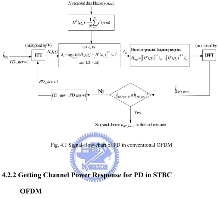
4.2.1 PD in Conventional OFDM………….………32

4.2.3 Diagonally Weighted STBC models……....……..……….38

4.2.4 PD in STBC OFDM……….………...42

4.2.5 Choice of received blocks window size in time-varying channel……44

5 Computer Simulations

47

5.1 Channel Estimate Error Performance……….………48

5.1.1 Subspace-based Method………...…48

5.1.2 Performance of PD………..53

5.1.3 Time-varying channel estimation………...………60

5.2 Bit Error Rate Performance………..………....63

5.3 Summary and the related work.………71

6 Conclusions

74

Appendix

76

Bibliography

79

List of Tables

2.1 Basic properties and comparisons between four-antenna STBCs………14

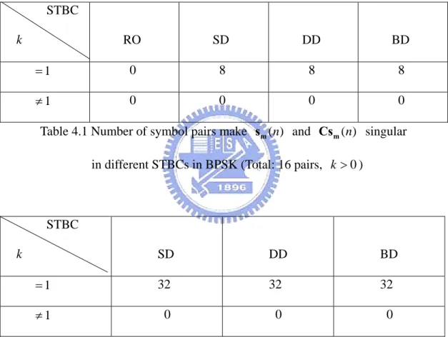
4.1 Number of symbol pairs make s_m( )n and Cs_m( )n singular in different STBCs in BPSK………..41

4.2 Number of symbol pairs make s_m( )n and Cs_m( )n singular in different STBCs in QPSK………..………..……41

List of Figures

2.1 Basic STBC transceiver model in frequency domain………....………….…5

3.1 Four-transmit-antenna STBC OFDM transceiver model with block precoders………16

3.2 Frequency domain version of four-antenna STBC OFDM transceiver model………..20

4.1 Signal-flow chart of PD in conventional OFDM…………....……..…………35

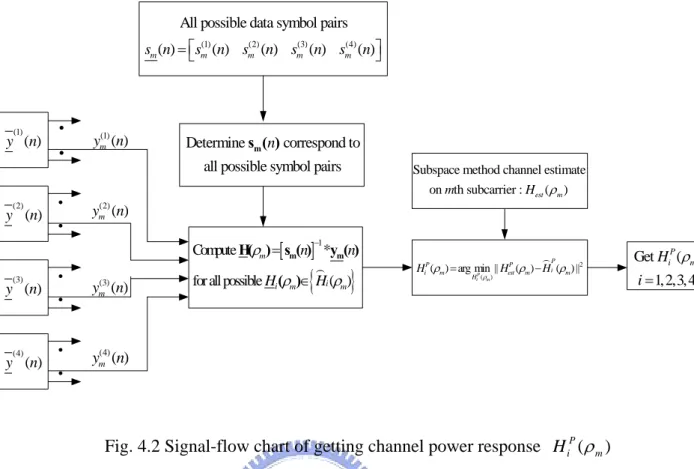
) 4.2 Signal-flow chart of getting channel power response H_iP(ρ_m in four-antenna STBC OFDM systems………..………38

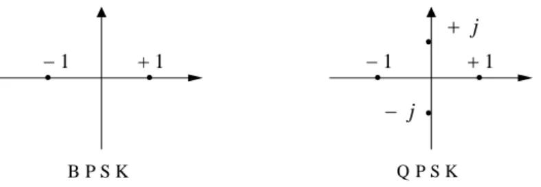
4.3 Signal constellations of BPSK and QPSK used in PD………..42

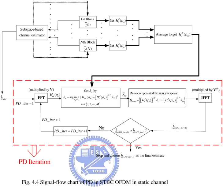
4.4 Signal-flow chart of PD in STBC OFDM in static channel...………...44

4.5 Signal-flow chart of PD in STBC OFDM in time-varying channel..…………46

5.1 RO & BD, Theoretical Subspace NMSCE………...……….49

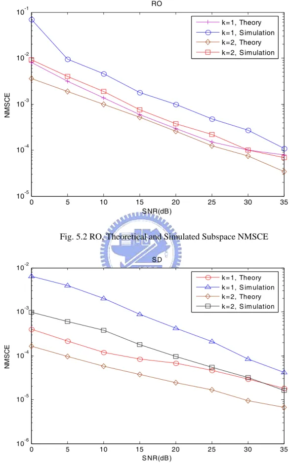
5.2 RO, Theoretical and Simulated Subspace……….………50

5.3 SD, Theoretical and Simulated Subspace…..……….……..………50

5.4 DD, Theoretical and Simulated Subspace………..………...51

5.5 BD, Theoretical and Simulated Subspace………..………...51

5.6 Four models, k =2 (k =1 for RO), Subspace…. ………52

5.7 RO, NMSCE vs. (SNR = 15 dB)………53 k 5.8 Four models, k =2 (k =1 for RO), Subspace + PD in BPSK……….…...54

5.9 Three models, k =2, Subspace + PD in QPSK……….………..54

5.10 RO, k=1, 2, Subspace & Subspace + PD in BPSK……….55

5.11 SD, k =2, Subspace & Subspace + PD in BPSK & QPSK………56

5.12 DD, k=2, Subspace & Subspace + PD in BPSK & QPSK………56

5.14 RO, , BPSK, Subspace & Subspace + PD with different multipath

lengths………..58

2 k= 5.15 SD, , BPSK, Subspace & Subspace + PD with different multipath lengths………..58

2 k= 5.16 DD, , BPSK, Subspace & Subspace + PD with different multipath lengths….……….59

2 k = 5.17 BD, , BPSK, Subspace & Subspace + PD with different multipath lengths………..59

2 k = 5.18 Four models, k =2, BPSK, Subspace with fd = 10Hz………60

5.19 Four models, k =2, BPSK, Subspace with fd = 50Hz………61

5.20 Four models, k =2, BPSK, Subspace with fd = 100Hz………..61

5.21 Four models, k =2, BPSK, Subspace with fd = 200Hz………..62

5.22 Four models, , BPSK, fd = 50Hz, Subspace & Subspace + PD (window size = 1, 50(RO, BD))………..……….63

2 k = 5.23 RO, BER vs. SNR (k=1, 2, 0.8)………...64 5.24 SD, BER vs. SNR (k=1, 2, 0.8)………64 5.25 DD, BER vs. SNR (k=1, 2, 0.8)………...65 5.26 BD, BER vs. SNR (k=1, 2, 0.8)………...65

5.27 Four models, BER vs. SNR (k=1)………..66

5.28 Four models, BER vs. SNR (k=2)………..67

5.29 RO, the effect of k on power of perturbations (SNR = 10, 15dB)………….70

5.30 BD, the effect of k on power of perturbations (SNR = 10, 15dB)………….70

5.31 Two different kinds of weighted BD, Subspace (k=2)………...72

Chapter 1

Introduction

Orthogonal frequency division multiplexing (OFDM) [1,2] has become a popular

technique for transmission of signals over wireless channels. It divides the whole

channel into many narrow parallel subchannels to increase the symbol period and

reducing or eliminating the inter-symbol interference (ISI) caused by the multipath

channel environment. The inter-channel interference (ICI), however, can be

eliminated by the independent and orthogonal among subcarriers, which is not easy to

obtain in practice. On the other hand, there is higher error probability for those

subchannels in deep fades since the dispersive property of wireless channels causes

frequency selective fading. Therefore, techniques such as error correction code and

diversity [2] have to be used to compensate for the frequency selectivity. In this thesis,

we investigate transmitter diversity using space-time block codes for OFDM systems.

Space-time block codes (STBC) [3-9] realize the diversity gains by applying

temporal and spatial correlation to the signals transmitted from different antennas

without increasing the total transmitted power and transmission bandwidth. They have

therefore been attractive means in high data rate transmissions. In fact, there is a

diversity gain that results from multiple paths between base station and user terminal,

and a coding gain that results from how symbols are correlated across transmit

antennas.

wireless communications, especially when receiver diversity is expensive or

impractical. Such systems always have more than one transmit-antenna and one

receive-antenna and are so-called multi-input single-output (MISO). With single

receive end, a well known two-transmit-antenna Alamouti STBC is proposed in [4]. In

this thesis, however, we want to look into four-transmit-antenna STBCs. Such model

includes real orthogonal [5], complex orthogonal [6,7], and complex non-orthogonal

[8,9]. In STBCs with more than two transmit antennas, real orthogonal models

guarantee full transmission rate (=1). But the complex orthogonal models cannot

achieve full rate [7]. The complex non-orthogonal ones, however, sacrifice the

orthogonality to achieve this goal [8,9].

For most STBC transceivers, multichannel estimation algorithms are important

issues. Training symbols are transmitted periodically in [10] for the receiver to

acquire the multi-input multi-output (MIMO) channels. However, training sequences

consume bandwidth and, thereby, incur spectral efficiency and capacity loss. For this

reason, blind channel estimation methods receive growing attention.

A few works have been proposed until now on blind MIMO and MISO channel

estimation that exploits the unique features of STBCs. Blind channel estimation and

equalization for MISO STBC systems has been proposed in [11] and for MIMO

STBC systems in [12,13]. Just like [14], [13] also introduced the semi-blind channel

estimation combining blind method and pilots. A subspace-based semi-blind method

is proposed in [15] for estimating the channel relying on redundant modulus

precoding responses.

In this thesis, unlike the similar system with two transmit antenna and Alamouti [4]

STBC proposed in [15], a linearly precoded STBC OFDM system with four transmit

antennas is introduced. Real orthogonal and complex non-orthogonal STBCs are

FIR channels through the subspace method is adopted as the channel estimation for

this system. Distinct redundant precoders insure that the subspace-based method can

estimate multiple channels simultaneously up to one scalar ambiguity [15]. The

theoretical mean square error of this estimator derived in [17] will also be mentioned

and be compared with the simulation results.

To further improve the subspace-based channel estimates, the “Phase direct (PD)”

method based on the finite alphabet property is exploited. The main idea of this

method is to solve the channel phase ambiguities after we have gained the channel

power response. PD originally works in conventional OFDM [16], which we can

acquire the channel power response easily by simple scalar division. But it is quite

different in STBC OFDM, since the received data consists of more than one different

transmitted data, which are not easy to be separated. So, the main problem we

encounter now is how to get the channel power response, which is practically hard to

obtain. In this thesis, the method of getting the channel power response for

four-antenna STBC OFDM is presented. The modulation classes we focus on are

BPSK and QPSK systems.

However, the singular transmission matrices produced by some possible symbol

pairs in non-orthogonal STBCs will make getting channel power response unworkable.

To solve this problem we modify the structure of transmission matrices of

non-orthogonal STBCs by multiplying a real constant gain on its diagonal

elements. Simulation results show that the increase of will better the subspace

estimator. But this will also increase noise power, which will make bit error rate

performance worse.

k

k

Furthermore, in time-varying channel, a proper window size of received data

blocks need to be chosen to get the channel power response and apply it to PD. A

system affected by noise more. The preorder form, however, is an issue that should

also be noticed behind the algorithm and will be discussed then.

This thesis is organized as follows. In Chapter 2, we show how data is transmitted

and received through space-time block code (STBC) and introduce several kinds of

STBCs. A novel kind of four-transmit-antenna complex non-orthogonal STBC named

Block Diagonal (BD) will be proposed. Four-antenna STBC combined with OFDM

system is presented in Chapter 3. A semi-blind channel estimation algorithm for

STBC OFDM and its improved method are shown in Chapter 4. Furthermore, Chapter

4 introduces the k -diagonally weighted transmission matrices for complex

non-orthogonal STBCs to prevent them from singular and therefore can be adopted in

PD. Chapter 5 exhibits simulation results and the effect of diagonal weight on

channel estimate error, noise, and bit error rate. Finally, our conclusions are

summarized in Chapter 6.

Chapter 2

Classifications of Space-Time Block

Codes

In this chapter, the basic concept of space-time block code (STBC) transceiving

process will be given first. We will then introduce several kinds of STBCs. Only the

first kind of STBC (Alamouti) is used in the 2-transmission-antenna system. Others

are used in 4-transmission-antenna systems, which can be divided into orthogonal and

non-orthogonal models. In complex non-orthogonal models, a novel kind of STBC

called Block Diagonal (BD) will be proposed. The structure of transmission matrix

and transceiving process of each STBC system will also be explained briefly.

2.1 Basic STBC tranceiving process

The following steps are all expressed in the frequency domain, as shown in Fig.2.1.

STBC Encoder

[

]

S

n

r

s

H

Suppose transmit antennas are used. STBC transmission matrix is presented as

. symbol vectors and their conjugates make up elements of

. Symbols in the same column of stand for symbols sent from the same transmit

antenna, while symbols in its same row stand for symbols sent in the same time slot. n

S n s1, s2, , sn

S S

The channel response vector is denoted by h, and the AWGN noise vector by n. h=

[

]

[

]

{

}

In the first place, modulated data symbols form the transmission matrices . Then

they are sent through channels. At the receiver end, received data symbol vector S

r can be presented as:

r S h n= * + (2.3) in frequency domain, where * is the matrix-vector multiplication.

In Eq. (2.3), AWGN are added after the symbols summed from different transmit

antennas in the same time slot. In the next step, r is adjusted to r so that only ' original data vectors s₁, s₂, s_n exist here in r after the adjustment. The ' terms of h_i and their conjugates are then exchanged with s_i. r can be written as: ' r' =H s n* + ' (2.4) where

s=

[

]

form its elements. Note that during Eq. (2.3) and Eq. (2.4), the characteristic of is

H h₁, h₂, , h_n

going to be transferred into H.

Finally, we can recover s from r by '

s H= −1*r'=H−1*H s H* + −1*n' = +s H−1*n' (2.6)

s is the soft decision data vector, which is at last sent into decision device to output

the hard decision data vector s.

2.2 Alamouti STBC

A simple STBC model had been proposed by Alamouti in [4]. The transmission

matrix of this scheme with two transmission antennas is

1_* 2_* (2.7) 2 1 s s s s ⎡ = ⎢−_{⎣ ⎦} S ⎤_⎥ 1

s and denote two transmitted symbol vectors that can be any size (including one). As we mentioned in section 2.1, the first and the second column of the matrix

denote the data symbol vectors transmitted by the first and the second antenna. While

the first and the second rows represent the two time slots it takes in a transmission

matrix to transmit the data vectors.

2

s

One of its important properties is that the transmission matrix is orthogonal. The

word “orthogonal” here means that the product matrix of the multiplication of S H and S is a diagonal matrix, where S is the Hermitian matrix (i.e. its transpose H conjugate matrix) of . Generally, each diagonal element of this product matrix

equals to . In this model: S Num_symbols 2 1 | i| i s =

∑

1 1 0 * 0 H a a ⎡ ⎤ = ⎢ ⎥ ⎣ ⎦ S S (2.8)

which corresponds to the definition of orthogonal, and

(2.9) 2 2 1 1 | i| i a s = =

∑

We also call SH*S the correlation matrix of S.

2.3 Four-by-four Orthogonal STBC

In this section, STBCs with four-by-four transmission matrices are introduced. Four

time slots are needed to transmit once (i.e. in a transmission matrix) and four transmit

antennas are used in these schemes.

2.3.1 Real Four-by-four Orthogonal (RO) STBC

As are the same in section 2.1, , , , and can denote four transmitted

symbol vectors of any size and form the transmission matrix. The STBC scheme

proposed in [5] transmits real symbols, such as PAM and BPSK. Its transmission

matrix is shown below:

1 s s₂ s₃ s₄ (2.10) 1 2 3 4 2 1 4 3 3 4 1 2 4 3 2 1 s s s s s s s s s s s s s s s s ⎡ ⎤ ⎢_{− −} ⎥ ⎢ = ⎢− ⎢_{− −} ⎥ ⎣ ⎦ S ⎥ ⎥ − 2 i s

S is also orthogonal. With real symbols, it is true that:

(2.11) Num_symbols Num_symbols 2 1 1 | _i| ( ) i i s = = =

∑

∑

0 ⎥ ⎥ Num_symbols 2 2 2 2 0 0 0 0 0 * 0 0 0 0 0 0 H a a a a ⎡ ⎤ ⎢ ⎥ ⎢ = ⎢ ⎢ ⎥ ⎣ ⎦ S S (2.12) where (2.13) 4 2 2 1 ( )i i a s = =

∑

Here, integer presents the number of transmitted symbol vectors in a

transmission matrix. The value of is 4 in this subsection. That means four

symbol vectors are sent during four time slots in a transmission matrix. So, the

transmission rate of this STBC is 1 and it is the maximum achievable transmission rate in a STBC system. In any arbitrary real signal system, there must exist STBC schemes that have maximum transmission rate with any number of transmission

antennas [7].

Num_symbols s_i

2.3.2 Complex Four-by-four Orthogonal (CO) STBC

In this subsection, the transmission matrix of STBC is also orthogonal. But the

complex modulation, such as QAM and PSK, is used. For any kind of complex

constellation, the maximal achievable transmission rate is

(

)

2 2 log _ log _ 1 2 N Tx N Tx ⎡ ⎤ ⎢ ⎥ + ⎡ ⎤ ⎢ ⎥ _{in an}

-transmit-antenna employed orthogonal STBC system [8]. Here, _

N Tx ⎡ ⎤_{⎢ ⎥}x means

the minimum integer larger than the real number x. For instance, the maximal

transmission rate for a 3 or 4-transmit-antenna system is 3/4. The transmission matrix

for a 2-antenna system (section 2.1), however, can always achieves the full

complex signals, it cannot achieve full rate for a STBC when . But for real

signals, however, full rate can be gained with any number of [7].

_ 3

N Tx≥ _ N Tx

The scheme introduced here, designed by Tarokh et al in [6,7], is a typical complex

four-by-four orthogonal STBC. A special feature of this scheme is that it only sends

three symbol vectors in every four time slots. Thus, its transmission rate is obviously

3/4, which corresponds to the fact mentioned above. Its transmission matrix structure

is: 3 3 1 2 * * 3 3 2 1 * * * * * * 3 3 1 1 2 2 2 2 1 1 * * * * * * 3 3 2 2 1 1 1 1 2 2 2 2 2 2 ( ) ( ) 2 2 2 2 ( ) ( ) 2 2 2 2 s s s s s s s s s s s s s s s s s s s s s s s s s s s s ⎡ ⎤ ⎢ ⎥ ⎢ ⎥ ⎢_{− −} ⎥ ⎢ ⎥ ⎢ ⎥ = − − + − − − + − ⎢ ⎥ ⎢ ⎥ ⎢ ⎥ ⎢ ₋ + + − ₋ + + − ⎥ ⎢ ⎥ ⎣ ⎦ S (2.14) and 3 3 3 3 0 0 0 0 0 * 0 0 0 0 0 0 H a a a a ⎡ ⎤ ⎢ ⎥ ⎢ = ⎢ ⎢ ⎥ ⎣ ⎦ S S 0 ⎥ ⎥ (2.15) where 3 2 3 1 | _i| i a s = =

∑

types.

2.4 Four-by-four Non-Orthogonal STBC

sacrifices in other properties of space-time block codes.

One of these sacrifices is that one may reduce the uncoded diversity gain, and rely

on coding to exploit the diversity provided by the additional antennas.

Another approach is that the requirement of orthogonality of the space-time block

code may be relaxed. Several designs of non-orthogonal space-time block codes will

be introduced in the following. With full transmission rate, these designs are also

based on 4 4× transmission matrices [8,9].

2.4.1 Spaced Diagonal (SD) STBC

This non-orthogonal (also called quasi-orthogonal) design was proposed by

Tirkkonen, Boariu and Hottinen in [8]. are four complex constellation

signals. The STBC transmission matrix is written as:

1, 2, ,3 4 s s s s ⎥ ⎥ 4⎥ ⎥ * 1 2 3 4 * * * * 2 1 4 3 3 4 1 2 * * * * 4 3 2 1 s s s s s s s s s s s s s s s s ⎡ ⎤ ⎢_{− −} ⎥ ⎢ = ⎢ ⎢_{− −} ⎥ ⎣ ⎦ S (2.17)

Thus, its correlation matrix is:

4 4 4 4 4 4 4 0 0 0 0 * 0 0 0 0 H a b a b b a b a ⎡ ⎤ ⎢ ⎥ ⎢ = ⎢ ⎢ ⎥ ⎣ ⎦ S S (2.18) where 4 2 4 1 | i| i a s = =

∑

4 S 4 ⎥ ⎥ ⎥ ⎥ *

Each of the non-orthogonal parts ( ) is separated by from the orthogonal parts

( ) in , so the name “Spaced Diagonal” is given. From the location of , we

can see that there are two non-orthogonal pairs in this model: the 1

4

b 0

a SH* b

st

and 3rd columns,

the 2nd and 4th columns.

2.4.2 Dual Diagonal (DD) STBC

Another work was proposed in [9] and developed the second kind of

non-orthogonal STBC. The transmission matrix is formed as:

(2.21) 1 2 3 4 4 3 2 1 * * * * 3 4 1 2 * * * * 2 1 4 3 s s s s s s s s s s s s s s s s ⎡ ⎤ ⎢ ⎥ ⎢ = ⎢ − − ⎢ _{− −} ⎥ ⎣ ⎦ S

Here, each same kind of symbol in forms a triangle in . The correlation

matrix of is: 1, 2, ,3 4 s s s s S S 5 5 5 5 5 5 5 5 0 0 0 0 * 0 0 0 0 H a b a b b a b a ⎡ ⎤ ⎢ ⎥ ⎢ = ⎢ ⎢ ⎥ ⎣ ⎦ S S (2.22) where 4 2 5 1 | _i| i a s = =

∑

located on the diagonal and reverse diagonal, respectively, in its correlation matrix.

2nd and 3rd columns.

2.4.3 Block Diagonal (BD) STBC

Here, we propose a novel kind of four-by-four non-orthogonal STBC named Block

Diagonal. Its may be generated by the general form in [12]. The transmission matrix

of this model is:

⎥ ⎥ ⎥ ⎥ * (2.25) 1 2 3 4 * * * * 3 4 1 2 2 1 4 3 * * * * 4 3 2 1 s s s s s s s s s s s s s s s s ⎡ ⎤ ⎢_{− −} ⎥ ⎢ = ⎢ ⎢_{− −} ⎥ ⎣ ⎦ S and (2.26) 6 6 6 6 6 6 6 6 0 0 0 0 * 0 0 0 0 H a b b a a b b a ⎡ ⎤ ⎢ ⎥ ⎢ = ⎢ ⎢ ⎥ ⎣ ⎦ S S where 4 2 6 1 | i| i a s = =

∑

pairs of SD and DD. Any two of four columns are in one non-orthogonal pair.

Therefore, three STBCs in section 2.4 have a total of different

non-orthogonal column pairs, which sit on all 12 non-diagonal locations of

(each occupies two). So these three STBCs contain all possible conditions of

4 2 6 C = * H S S

non-orthogonal STBCs with two non-orthogonal pairs.

2.5 Summary

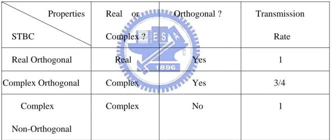
Comparing to the Complex Orthogonal STBC in the same transmission matrix size,

the Complex 4-by-4 Non-orthogonal STBCs have poor SER/BER performances at

low SNR (< 15dB) [8,9] and more complicated equalization matrices at the receive end, in the trade off of higher transmission rate. The basic properties and comparisons

of four-antenna STBCs introduced in this chapter are shown in Table. 2.1.

Properties STBC Real or Complex ? Orthogonal ? Transmission Rate

Real Orthogonal Real Yes 1

Complex Orthogonal Complex Yes 3/4

Complex

Non-Orthogonal

Complex No 1

Table 2.1 Basic properties and comparisons between four-antenna STBCs

In chapter 3, we will demonstrate how these four-antenna STBCs are combined

with the OFDM system. In chapter 4, channel estimation methods for STBC OFDM

in chapter 3 will be given. Four types of four-antenna STBC models: RO, SD, DD,

Chapter 3

Space-Time Block Code OFDM

System Model

We will combine STBCs with OFDM system in this chapter. The system we use in

this thesis is similar to that in [15,17], which has two transmit antennas, one receive

antenna, and Alamouti STBC (section 2.2).

Four transmit antennas are used here in this system, and its model is depicted in Fig.

3.1. Any kind of schemes in section 2.3 and section 2.4 can be chosen as the STBC in

this OFDM system.

The symbols are divided into huge block vectors first with size before

transmission. Each block is further separated into four smaller parts with each has

symbols.

4K×1

K

(1)

( )

s n denotes the first K symbols of s n( ), while s(2)( )n , s(3)( )n ,

(4)

( )

s n denotes its second, third, and last K symbols.

(1) (2) (3) (4) ( ) ( ) ( ) ( ) ( ) s n s n s n s n s n ⎡ ⎤ ⎢ ⎥ ⎢ = ⎢ ⎢ ⎥ ⎢ ⎥ ⎣ ⎦ ⎥ ⎥ (3.1)

With each one of size M× ( M KK > ), four different tall matrices , , and (for input block symbols

1 θ θ₂ θ₃ 4 θ (1) ( ) s n , s(2)( )n , s(3)( )n , and s(4)( )n , respectively)

represent four distinct linear block precoders where s n( ) is first sent to. After

precoders, the input symbol block becomes

(1) (1) (1) 1 (2) _{(2) (2)} (3) (3) (3) (4) (4) (4) ( ) _{( ) ( )} ( ) ( ) ( ) ( ) ( ) ( ) ( ) ( ) ( ) ( ) ( ) s n _{s n s n} s n s n s n s n s n s n s n s n s n s n s n ⎡ _{⎤ ⎡ ⎤ ⎡ ⎤} ⎡ ⎤ ⎢ _{⎥ ⎢ ⎥ ⎢ ⎥} ⎢ ⎥ ⎢ _{⎥ ⎢ ⎥ ⎢ ⎥} ⎢ ⎥ ⎢ ⎥ = =_{⎢ ⎥}= _{⎢ ⎥}= ⎢ ⎥ ⎢ _{⎥ ⎢ ⎥ ⎢ ⎥} ⎢ ⎥ ⎢ _{⎥ ⎢ ⎥ ⎢ ⎥} ⎣ ⎦ ⎢ ⎥ ⎣ ⎦ ⎣ ⎦ ⎣ ⎦ 1 2 2 3 3 4 4 θ _{θ 0 0 0} θ 0 θ 0 0 Θ 0 0 θ 0 θ 0 0 0 θ θ (3.2) where (3.3) ⎡ ⎤ ⎢ ⎥ ⎢ = ⎢ ⎢ ⎥ ⎣ ⎦ 1 2 3 4 θ 0 0 0 0 θ 0 0 Θ 0 0 θ 0 0 0 0 θ ⎥ ⎥

is a 4M×4K matrix and ( )s n is of size 4M× . 1

STBC Encoder 1 2 3 4 , , θ θ θ θ ( ) s n s n( ) 1( ) s n 2( ) s n 3( ) s n 4( ) s n IFFT W IFFT W IFFT W IFFT W 1( ) u n 2( ) u n 3( ) u n 4( ) u n P/S P/S P/S P/S 4( ) u n 3( ) u n 2( ) u n 1( ) u n CP A CP A CP A CP A Tx1 Tx2 Tx3 Tx4 ∑ Rx ( ) w n 1 h 2 h 3 h 4 h S/P CP R ( ) y n ( ) y n ( ) y n FFT W

( )

3.1 STBC Encoder and Transmitter

( )

s n is then sent to the space-time encoder. Any four-antenna STBC can be used

to in the system. The four precoded sub-blocks of ( )s n : s(1)( )n , s(2)( )n , s(3)( )n ,

and s(4)( )n will form a 4M× output code matrix of encoder as 4

(1) (1) (1) (1) 1 2 3 4 (2) (2) (2) (2) ( ) 1 2 3 4 1 2 3 4 _{(3) (3) (3) (3)} 1 2 3 4 (4) (4) (4) (4) 1 2 3 4 ( ) ( ) ( ) ( ) ( ) ( ) ( ) ( ) ( ) ( ) ( ) ( ) ( ( )) ( ) ( ) ( ) ( ) ( ) ( ) ( ) ( ) i s n s n s n s n s n s n s n s n s n s n s n s n s n s n s n s n s n s n s n s n s n ⎡ ⎤ ⎢ ⎥ ⎢ ⎥ ⎢ ⎥ ⎡ ⎤ = = ⎣ ⎦ ⎢ ⎥ ⎢ ⎥ ⎢ ⎥ ⎢ ⎥ ⎣ ⎦ M =S (3.4)

where i=1, 2,3, 4. s_i(1)( )n , s_i(2)( )n , s_i(3)( )n and s_i(4)( )n are all OFDM symbol. is the transmission matrix of STBC in chapter 2. Eq. (3.4) shows that the blocks in S

( )

s n in Eq. (3.2) are transmitted through four different independent channels in four consecutive time intervals.

After the OFDM symbols encoded by the space-time encoder, they are modulated

by M-point IFFT, where the result equals to multiplied by an IFFT matrix .

Vectors

IFFT W

( )

i

u n are produced (i=1, 2, 3, 4), then.

The size of time domain symbol vector u n is then be expanded by a length i( ) cyclic prefix (CP) to eliminate the effect of inter-block-interference (IBI) caused by

channel, and its size becomes

L

M + , then. The CP of L W_Ms_i( )l ( )n is the replicas of its last L elements and will be put in front of it, where l=1, 2, 3, 4. The channel order ((number of channel taps) 1− ) is assumed to be less than or equal to . The L

insertion of CP is represented by A_CP in Fig. 2.1, and the outputs are u ni( ). They

are finally sent through transmit antenna sequentially, i i=1, 2, 3, 4.

3.2 Channel

In the following descriptions, the channels between four transmit antennas and the

receive antenna are assumed to be frequency selective and their discrete time

baseband equivalent effect is in the form of the FIR linear time-invariant filter, which

has the impulse response vector

h_i =[ (0), (1),h_i h_i …, ( )] , h L_i T i=1, 2, 3, 4 L

(3.5)

where L≥max( ,L L L_{1 2}, ₃, ₄). L_i is the channel order of h , 1, 2,3, 4_i i= .

The FIR channel H_i is a (M +L)×(M +L) lower-triangular Toeplitz matrix and its ( , )s t th element is h s ti( − ), s t, ∈

{

}

3.3 Receiver

At the receiver end, an additive white Gaussian noise vector w n( ) is added to the

I

received symbols. The removing of CP can be described by the

matrixR_CP =[0_{M L× M}]. And the matrix Hi represents the equivalent channel

matrix without IBI, where

i = _{CP i CP}

H R H A (3.7) In Fig. 3.1, the received IBI-free 4M× block ( )1 y n can be written as:

(1) (2) (3) (4) ( ) ( ) ( ) ( ) ( ) y n y n y n y n y n ⎡ ⎤ ⎢ ⎥ ⎢ = ⎢ ⎢ ⎥ ⎢ ⎥ ⎣ ⎦ ⎥ ⎥ (3.8)

After removing the CP, the OFDM symbols in y n are demodulated by M-point ( ) FFT, which is presented as being multiplied by the M×M FFT matrix to obtain the received block

FFT W ( ) y n , (1) (2) (3) (4) ( ) ( ) ( ) ( ) ( ) y n y n y n y n y n ⎡ ⎤ ⎢ ⎥ ⎢ ⎥ = ⎢ ⎢ ⎥ ⎢ ⎥ ⎣ ⎦ ⎥ (3.9) We then adjust y n to ( )( ) y n by * * (1) (2) (3) (4) ( ) ( ) ( ) ( ) ( ) y n y n y n y n y n ⎡ ⎤ ⎢ ⎥ ⎢ ⎥ = ⎢ ⎢ ⎥ ⎢ ⎥ ⎢ ⎥ ⎣ ⎦ ⎥ (3.10)

and sent to space-time decoder. The output z n( ) is a block with diversity gain. After

all, the original data symbol s n( ) is recovered from z n( ) by applying the equalizer

.

Γ s n is the soft decision data here, which is perturbed by the noise. It is then put ( )

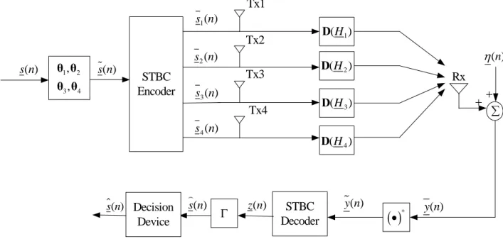
version of Fig. 3.1 can then be plotted in Fig. 3.2. STBC Encoder 1 2 3 4 , , θ θ θ θ ( ) s n s n( ) 1( ) s n 2( ) s n 3( ) s n 4( ) s n Tx1 Tx2 Tx3 Tx4 1 (H ) D 2 (H ) D 3 (H ) D 4 (H ) D ∑ Rx ( )n η + + ( ) y n STBC Decoder ( ) z n Γ ( ) s n Decision Device ( ) s n y n( )

( )

Fig. 3.2. Frequency domain version of four-antenna STBC OFDM transceiver model

The frequency response vector of channel h in Eq. (3.6) is_i

Hi = Vh (3.11) i

with matrix V is the submatrix of the first L+ columns of 1 W_FFT .

The equivalent channel matrix in time domain Hi can be diagonalized by pre- and

post-multiplication with W_FFT and W_IFFT:

W_FFTH Wi _IFFT =D(H_i) (3.12)

where D(Hi) denoting the diagonal matrix with Hi on its diagonal.

Combining the fact above, Eq. (3.4) and Eq. (3.9) together, we can rewrite y n ( )

4 (1) 1 4 (2) 1 4 (3) 1 4 (4) 1 ( ) ( ) ( ) ( ) ( ) ( ) ( ) ( ) ( ) ( ) i i i i i i i i i i i i H s n H s n y n H s n H s n = = = = ⎡ _{⎡ ⎤}⎤ ⎢ ⎣ ⎦⎥ ⎢ ⎥ ⎢ _{⎡ ⎤}⎥ ⎢ ⎣ ⎦⎥ ⎢ = ⎢ ⎥ ⎡ ⎤ ⎢ ⎣ ⎦⎥ ⎢ ⎥ ⎢ ⎥ ⎡ ⎤ ⎢ _{⎣ ⎦}⎥ ⎣ ⎦

∑

∑

∑

∑

3.4 STBC Decoder and Equalizer

Here, let us take BD in section 2.4.3 for example, Eq. (3.10) can be written as:

* * (1) (2) (3) (4) ( ) ( ) ( ) ( ) ( ) y n y n y n y n y n ⎡ ⎤ ⎢ ⎥ ⎢ ⎥ = ⎢ ⎥ ⎢ ⎥ ⎢ ⎥ ⎢ ⎥ ⎣ ⎦ * * (1) ₍₁₎ 1 2 3 4 (2) * * * * (2) 3 4 1 2 (3) (3) 2 1 4 3 * * * * (4) (4) 4 3 2 1 ( ) ( ) ( ) ( ) ( ) ( ) ( ) ( ) ( ) ( ) ( ) ( ) = ( ) ( ) ( ) ( ) _{( ) ( )} ( ) ( ) ( ) ( ) _{( )} ( ) s n v n H H H H H H H H s n v n H H H H _{s n v n} H H H H _{v n} s n ⎡ _{⎤ ⎡} ⎡ _{⎤ ⎢ ⎥ ⎢} ⎢ _{⎥ ⎢ ⎥ ⎢} − − ⎢ _{⎥ ⎢ ⎥ + ⎢} ⎢ _{⎥ ⎢ ⎥ ⎢} ⎢ _{⎥ ⎢ ⎥ ⎢} ⎢ − − ⎥ ⎣ ⎦ ⎢_{⎣ ⎥ ⎣⎦} D D D D D D D D D D D D D D D D = s n( ) η( )n s n( ) η( )n x n( ) η( )n ⎤ ⎥ ⎥ ⎥ ⎥ ⎥ ⎦ + = + = + D Θ A (3.15) where 1 2 3 4 * * * 3 4 1 * 2 1 4 3 * * * 4 3 2 1 ( ) ( ) ( ) ( ) ( ) ( ) ( ) ( ) ( ) ( ) ( ) ( ) ( ) ( ) ( ) ( ) H H H H H H H H H H H H H H H H ⎡ ⎤ ⎢ ⎥ − − ⎢ ⎥ = ⎢ ⎥ ⎢ ⎥ ⎢ − − ⎥ ⎣ ⎦ D D D D D D D D D D D D D D D D 2 * D , * * (1) (2) (3) (4) ( ) ( ) ( ) ( ) ( ) v n v n n v n v n η ⎡ ⎤ ⎢ ⎥ ⎢ ⎥ =⎢ ⎥ (3.16) ⎢ ⎥ ⎢ ⎥ ⎣ ⎦

A D= Θ, x n( )= A ns( ) (3.17) If the frequency domain channel state vectors H1, H2, H3 and H4 are

available at the receiver, z n( ) can be obtained from y n by: ( )

( ) ( ) ( ) ( ) ( ) ( ) H H z n y n s n n s n n η ξ = = + = _A + D D D Θ D D H (3.18) where H = A D D D Θ (3.19) and ξ( )n = DHη( )n (3.20) In above equations, the decoding step D D comes from H of STBCs in chapter 2. Eq. (3.10) will turn the property of orthogonal (or non-orthogonal) of

STBCs from into

*

H S S

S D . So the correlation matrix can be used in decoding, for

simplification. Note that it has been achieved multiantenna diversity of order four.

From Eq. (3.18), we know that D_AH and the inverse of

(

)

(

)

4K =

A

D in Eq. (3.19) should be full column rank (=4K), which means every M×M submatrix in D_A (except 0: M×K) must be full column rank (=4K).

So the designing of precoders is a main issue. Two important conditions in [15]

should be taken into consideration, here: Condition (3.1) M > + . K L

independent.

The form of precoders will be mentioned later in chapter 5.

After going through the equalizer Γ , the output is the soft decision data:

(

)

(

)

(

)

(

)

finite alphabet to get the hard decision data s n( ).

The channel state information (CSI) in Eq. (3.19) is assumed to be perfectly

available at the receiver end. In the next chapter, we will exhibit how to get the

Chapter 4

Subspace-based Channel

Estimation and the improved

method Phase Direct

In four-antenna STBC OFDM systems, the channel estimation method is based on

the redundancy caused by four M× linear precoders , K , , and , which is similar to the channel estimation in the two-antenna system in [17].

1

θ θ2 θ3 θ4

We will first simply describe the main idea of the subspace-based channel

estimation. Similar or same methods had been proposed for some two and

four-antenna STBCs in [11-14,15,17]. After the description, the design of precoders in

our systems is introduced. The theoretical mean square error of this algorithm derived

in [17] will then be mentioned.

In section 4.2, an improved finite alphabet method based on the subspace-based

channel estimation named phase direct (PD) [16], will be introduced to make the

channel estimates better. The PD based on subspace method in [17] only focus on

Alamouti STBC [4] with BPSK modulation. Here, we will extend it to four-antenna

STBC OFDM systems in section 2.3.1 and 2.4. We will also extend all these three

systems from BPSK modulation to QPSK modulation, which will also result in more

issue in PD. Such issue in the two-antenna Alamouti STBC OFDM system with

BPSK was also mentioned in [17]. In four-antenna STBC OFDM systems, because

the possible conditions of channel power response become more, the getting of the

channel power response is more complicated than that in a two-antenna system. And

so is that in QPSK than in BPSK in the same system. The algorithm we use in this

thesis to get channel power response is to select the most proper one from all its

possible conditions. So we should find out all the possible conditions of its channel

power response. Such algorithm is going to be discussed in section 4.2.2.

Furthermore, the feasibility for the algorithm in section 4.2.2 depends on that all

possible symbol conditions for of STBCs are non-singular. To achieve this goal,

we will introduce the diagonally weighted models of STBCs in section 4.2.3. PD for

four-antenna STBCs in static channel will be expressed in section 4.2.4. S

Finally, in time-varying channel, the choice of window size of received blocks in

PD will also be mentioned. This will be shown in section 4.2.5 while the same issue

was also taken in [17]. A longer window of received blocks can lessen the effect of

noise but cannot follow the varying channel, while a shorter window can follow the

channel variance more precisely than a longer one.

4.1 Subspace-based Multichannel Estimation

In the following description in this method, as the same in chapter 3, we also

choose Block Diagonal (BD) STBC in 2.4.3 to show the estimation algorithm here.

4.1.1 Subspace-based Multichannel Estimation Method

First, the algorithm starts from the received data vectors in Eq. (3.17), neglecting

y n( )=x n( )= As n( ) (4.1) N blocks of ( )y n =x n( ) are collected and form a matrix X_N in the size 4M×N:

[

]

where

SN =

[

]

It is impossible to implement this algorithm on the Complex Orthogonal (CO)

STBC system in section 2.3.2, however, because its received data vectors ( )y n cannot be presented in the form of As n( ) in Eq. (4.1) [11].

Compared to the condition in the two-antenna system in [15,17] that the number of

received blocks should be large enough ( ). must satisfy the condition

that here in four-antenna systems to guarantee that is with full rank

.

N ≥2K N

4

N≥ K S_N

4K

According to Condition (3.1), Condition (3.2), and the condition above. s n( ), a independent data vector, will show the fact that

4K×1 rank(X_N)=4K, and that the

nullity of X_N null(X_N)=4M−4K . Note that the range space of . So the singular value decomposition (SVD) of can

be written as: N X ( _N) ( _N H_N) ( R X =R X X =R A) X_N

[

]

∑

where

∑

2 2

1 2 k

2 4

σ ≥σ ≥ ≥σ . The null eigenvalues (all zeroes) yield null eigenvectors of , which form the 4

N X

(4 4 )

M× M− K matrix and column span the null space caused by redundant preorders.

n U

( _N N X )

Next, we use the property that N X( N) is orthogonal to R(XN)=R( )A , it appears

that:

ukHA=0, k =1, 2, , 4M −4K (4.5)

where u is the th column of the null space matrix _k . It is also the th null eigenvector of .

k U_n k

N X

Then, we separate the 4M× 1 u into four equal size parts: k

_1 _ 2 _ 3 _ 4 k st k nd k k rd k th u u u u u ⎡ ⎤ ⎢ ⎥ ⎢ =_⎢ ⎢ ⎥ ⎢ ⎥ ⎣ ⎦ ⎥ ⎥ (4.6)

where all of its four parts are M× vectors. 1

Here, we take BD in OFDM for example. By Eq. (3.15) and Eq. (4.5), it can be

shown that 1 2 3 4 * * * * 3 4 1 2 _1 _ 2 _ 3 _ 4 2 1 4 3 * * * * 4 3 2 1 ( ) ( ) ( ) ( ) ( ) ( ) ( ) ( ) ( ) ( ) ( ) ( ) ( ) ( ) ( ) ( ) 0 H k H H H H k st k nd k rd k th u H H H H H H H H u u u u H H H H H H H H ⎡ _{⎤ ⎡ ⎤} ⎢ _{⎥ ⎢ ⎥} − − ⎢ _{⎥ ⎢ ⎥} ⎡ ⎤ = ⎣ ⎦ ⎢ _{⎥ ⎢ ⎥} ⎢ _{⎥ ⎢ ⎥} ⎢ − − ⎥⎣ ⎦ ⎣ ⎦ = 1 2 3 4 A D D D D _{θ 0 0 0} 0 θ 0 0 D D D D 0 0 θ 0 D D D D 0 0 0 θ D D D D (4.7)

For any M× vectors 1 a and b, it is true that

aHD( )b =bD(a*) (4.8) where D(*) is as defined in chapter 3.

* * _1 _ 3 _ 2 _ 4 * * _ 3 _1 _ 4 _ 2 1 2 3 4 * * _ 2 _ 4 _1 _ 3 * * _ 4 _ 2 _ 3 _1 ( ) ( ) ( ) ( ) ( ) ( ) ( ) ( ) ( ) ( ) ( ) ( ) ( ) ( ) ( ) ( ) ( ) k k st k rd k nd k th k rd k st k th k nd T T H H k nd k th k st k rd k th k nd k rd k st u u u u u u u u u H H H H u u u u u u u u = ⎡ − − ⎤ ⎢ ⎥ − − ⎢ ⎥ ⎡ _{⎤ ⎢ ⎥} ⎣ ⎦ ⎢ ⎥ ⎢ ⎥ ⎣ ⎦ G D D D D D D D D D D D D D D D D * 3 * 4 0 ⎡ ⎤ ⎢ ⎥ ⎢ _{⎥ =} ⎢ ⎥ ⎢ ⎥ ⎣ ⎦ 1 2 =Ψ θ 0 0 0 0 θ 0 0 0 0 θ 0 0 0 0 θ (4.9) where * * _1 _ 3 _ 2 _ 4 * * _ 3 _1 _ 4 _ 2 * * _ 2 _ 4 _1 _ 3 * * _ 4 _ 2 _ 3 _1 ( ) ( ) ( ) ( ) ( ) ( ) ( ) ( ( ) ( ) ( ) ( ) ( ) ( ) ( ) ( ) ( ) k st k rd k nd k th k rd k st k th k nd k k nd k th k st k rd k th k nd k rd k st u u u u u u u u u u u u u u u u u ⎡ − − ⎤ ⎢ ⎥ − − ⎢ ⎥ = ⎢ ⎥ ⎢ ⎥ ⎢ ⎥ ⎣ ⎦ D D D D D D D D G D D D D D D D D ) ⎥ ⎥ (4.10) and _* (4.11) 3 * 4 ⎡ ⎤ ⎢ ⎥ ⎢ = ⎢ ⎢ ⎥ ⎣ ⎦ 1 2 θ 0 0 0 0 θ 0 0 Ψ 0 0 θ 0 0 0 0 θ

Using the relationship between h and _i H_i in Eq. (3.11), Eq. (4.9) is transformed into _{1 2 3 4} ( ) 0 T T T T H H k H H h h h h u = ⎡ ⎤ ⎢ ⎥ ⎢ ⎥ ⎡ ⎤ = ⎣ _{⎦ ⎢ ⎥} ⎢ ⎥ ⎣ ⎦ F V 0 0 0 0 V 0 0 G Ψ 0 0 V 0 0 0 0 V (4.12) where (4.13) T T H H ⎡ ⎤ ⎢ ⎥ ⎢ = ⎢ ⎢ ⎥ ⎣ ⎦ V 0 0 0 0 V 0 0 F 0 0 V 0 0 0 0 V ⎥ ⎥

In Eq. (4.12), the channel states are presented in time domain rather than in frequency

rows (4(L+1)) than G(uk)Ψ has ( 4M ), and it can thus reduce computation complexity.

Now, we have every null eigenvector u in Eq. (4.5) doing all the steps above, k

with k=1, 2, , 4M −4K. And then put them in a row, we can get

_{1 2 3 4}

[

]

The zero vector 0 here in Eq. (4.14) has 1 row and 4(L+ ×1) [4K×(4M −4 )]K columns, and hH = ⎣⎡h₁T h₂T h₃H h₄H⎤⎦ (4.15) Q F G=

[

]

which corresponds to the smallest eigenvalue of QQH:

{

}

By Eq. (4.15), the estimated channel is

* 1 * 2 3 4 h h h h h ⎡ ⎤ ⎢ ⎥ ⎢ ⎥ = ⎢ ⎥ ⎢ ⎥ ⎢ ⎥ ⎣ ⎦ (4.19)

This algorithm is named subspace-based channel algorithm since it is based on the

null space U_n of received data matrix X_N.

However, in the realistic condition, the white noise is added at the receiver end. In

~ ~ ~ ~ ~ _~ H x x x n N _H n n ⎡ ⎤_{⎡ ⎤} ⎢ ⎥ ⎡ ⎤_{⎢ ⎥}⎢ ⎥ = ⎢_⎣ ⎥_{⎦⎢ ⎥}⎢ ⎥ ⎢ ⎥ ⎢ ⎥ ⎣ ⎦ ⎣ ⎦

∑

∑

The diagonal matrix

~

x

∑

x

∑

(4.4), also has range eigenvalues of in its diagonal elements. , however,

will have the variance of white noise on its diagonal [15].

N X N

Y

∑

As it mentioned in [15,17], in order to simplify the computation, we replace in

Eq. (4.20) by the sample covariance matrix of

N Y ( ) y n in Eq. (3.15): 1 1 ( ) ( ) N _H y n y n y n N = =

∑

1 2 3 4 0

T T H H

h h h h

⎡ =

⎣ ⎤⎦Q in Eq. (4.14) is not unique. According to the description about channel identifiability in [15], if distinct precoders (any of the four precoders is

different from each other) are used, channel identifiability within one scalar α is guaranteed. For example:

1 ₁ 2 * 3 3 * 4 4 h _h h h h h h h α α α α ⎡ ⎤ 2 ⎡ ⎤ ⎡ ⎤ ⎢ ⎥ _{⎢ ⎥⎢ ⎥} ⎢ ⎥ _{⎢ ⎢ ⎥} = ⎢ ⎥ _⎢ ⎥_{⎢ ⎥} ⎢ ⎥ _⎢ ⎥_{⎥⎢ ⎥} ⎢ ⎥ ⎣ ⎦ ⎣ ⎦ ⎣ ⎦ I 0 0 0 0 I 0 0 0 0 I 0 0 0 0 I (4.22)

holds true in BD, where h is the final estimate of channels, i i=1, 2,3, 4. Here, we

use one pair of pre-precoding pilots in [15] to resolve the unknown scalar α .

Other three four-antenna STBCS, however, can also be adopted in the proposed

subspace-based channel estimation algorithm. The major steps of this algorithm in

Step 1) Collect N received data blocks y n and compute ( ) R_y in Eq. (4.21). Note that N ≥4K is the necessary condition in four-antenna systems.

Step 2) Find out the eigenvectors u ,_k k=1, 2, , 4M −4K, corresponding to the smallest 4M −4K eigenvalues of the matrix R_y, by proceeding its SVD. Step 3) Build Q in Eq. (4.16).

Step 4) Determine the eigenvector corresponding to the smallest eigenvalue of QQH

in Eq. (4.18) as the initial estimate.

Step 5) Resolve the scalar ambiguity α and determine the final estimate of channels.

4.1.2 Theoretical Mean Square Error of subspace method

[17]. For high SNR and large sample size (large N ), an approximation MSE is

2 2 2 2 2 (|| || ) (|| || ) ( ) ( ) || || = H H w w s s E h h E h E trace h h trace N N σ σ σ σ + + 2 + 2 ⎡ ⎤ − = = _⎣ ⋅ _⎦ ⋅ ≈ Q Q ⋅ Q (4.23)

This formula can be adopted in four-antenna systems as well as in the two-antenna

system. h is the estimate of channels and h is the real one. Both signals and noise

are assume to be i.i.d random variables with zero mean and variance σ_s2 and σ_w2, respectively. So we get σ σ_s2/ _w2 as SNR. is the number of sampling received data blocks. And the matrix

N

+

Q , which comes from Q in Eq. (4.16), will be explained as follows: With noise is added, assuming Q permits the SVD

~ ~ ~ ~ ~ _~ H q q q nq H nq nq ⎡ ⎤_{⎡ ⎤} ⎢ ⎥ ⎡ ⎤_{⎢ ⎥}⎢ ⎥ = ⎢_⎣ ⎥_{⎦⎢ ⎥}⎢ ⎥ ⎢ ⎥ ⎢ ⎥ ⎣ ⎦ ⎣ ⎦

∑

∑

where Q+ is computed as 1 ~ ~ ~ H q _q − + ₌ ⎛ ⎞ ⎜ ⎟ ⎝

∑

4.2 Phase Direct (PD)

PD was proposed in conventional (SISO) OFDM [16]. It was then addressed to

Alamouti STBC OFDM ([4], section 2.2) in [17]. In this thesis, we will combine it

with four-antenna STBC OFDM systems, and based on subspace method to improve

channel estimation.

4.2.1 PD in Conventional OFDM

We first show how PD performs in conventional OFDM. The signal modulation

types in discussion are P-'ary PSK constellations with size

{

}

: _P j p P| 1, 2, P ξ =e π p= , P

m

, here. In convention OFDM, the signal at the receive

end can be written as

y n m( , )=H(ρ_m) ( , )s n m +n(ρ ) (4.26) where s n m( , ) and y n m are the transmitted and received data signals, ( , ) respectively, through the th subcarrier on the th received data block. is

in the form of .

m n s n m( , )

P H(ρ_m) is the channel response of the th subcarrier in frequency domain and

m

( _m)

n ρ is the corresponding noise. A total of M subcarriers and N received data blocks are taken.

For the simplification of getting the power of to signal in Eq. (4.26), we neglect

the noise, and take the expectation to :

P n