非同步雙向圓環面連結網路

國

立

交

通

大

學

資訊科學與工程研究所

碩

士

論

文

非同步雙向圓環面連結網路

Asynchronous Interconnection Network using Torus Topology

研 究 生：蔡嘉承

指導教授：陳昌居 教授

非同步雙向圓環面網路連結

Asynchronous Bi-direction Interconnection Network Implementation

using Torus Topology

研 究 生：蔡嘉承 Student：Chia-Cheng Tsai

指導教授：陳昌居 Advisor：Chang-Jiu Chen

國 立 交 通 大 學

資 訊 科 學 與 工 程 研 究 所

碩 士 論 文

Submitted to Institute of Computer Science and Engineering College of Computer Science

National Chiao Tung University in partial Fulfillment of the Requirements

for the Degree of Master

in

Computer Science

June 2009

Hsinchu, Taiwan, Republic of China

i

非同步雙向圓環面連結網路實作

學生：蔡嘉承 指導教授：陳昌居教授

國立交通大學

資訊科學與工程研究所

摘要

ii

Asynchronous Bi-direction Interconnection Network

Implementation using Torus Topology

Student: Chia-Cheng Tsai Advisor: Prof. Chang-Jiu Chen

Department of Computer Science and Information Engineering

National Chiao Tung University

Abstract

NOC is a popular topic in recent year, and how to efficiency to connect processors with

different frequency are very hard. But, if we use asynchronous circuits design and torus

system, the problems can be solved easily. In asynchronous circuits, it uses handshaking to

replace the clock to synchronous every sub-circuits, and the torus system uses extra data paths

to reduce the transfer time. We use packet-switching and the new algorithms to avoid the

deadlock and make sure the packet sequence. By simulation, the packets spend about 40000ps

to pass through one router, and there would not cause deadlock happen when the system is

iii

Acknowledgement

iv

CONTENTS

Chapter 2 Related Works……….3

2.1 Asynchronous Circuit Design………3

2.1.1 Advantages………...3 2.1.2 Handshaking protocol……….……….5 2.2 Interconnection Networks………...9 2.2.1 Shared Bus……….………9 2.2.2 Net………11 2.2.3 Mesh………12 2.2.4 Torus system………13 2.2.5 Comparison………14 2.3 Data Transfer………...18 2.3.1 Wormhole………18 2.3.2 Packet-switching………...19 2.3.3 Deadlock……….20 2.3.4 Starvation………20 2.3.5 Comparison………20 2.4 C-element………..21

v Chapter 3 Design………...23 3.1 Data Flow………..……….24 3.2 System………...26 3.3 Routing Algorithm………..………...31

3.3.1

3.3.2

3.3.3

3.5.1

3.5.2

3.5.3

3.5.4

3.5.5

Chapter 5 Conclusion and Future Works………59

vi

Lists of Figures

Figure 1 (a) Bundle data channel………6

Figure 1 (b) Four-phase protocol………..………6

Figure 2 (a) Dual-rail………...8

Figure 2 (b) Dual-rail protocol………8

Figure 3 Transfer diagram………...……9

Figure 4 Sharing Bus……….10

Figure 5 The Net system……….11

Figure 6 The Mesh system………..……13

Figure 7 The torus system………14

Figure 8 The data paths of Mesh system………...16

Figure 9 The data paths of uni-direction torus system………16

Figure 10 The data paths of Bi-direction torus system…..………16

Figure 11 (a) C-element……...……….22

Figure 11 (b) C-element with RESET……….22

Figure 12 Data Flow (1)………24

Figure 13 Data Flow (2)…...……….25

Figure 14 Router’s Architecture………26

Figure 15 The torus system………...………28

Figure 16 Transfer order 1………30

Figure 17 Transfer order 2………30

Figure 18 Algorithm 1: Arrival……….………31

Figure 19 Algorithm 2: Direct-decision………33

Figure 20 Algorithm 3: Head-building………..………34

vii

Figure 22 (a) Data format………..………38

Figure 22 (b) Data format……….………38

Figure 23 (a) HEAD………..………38

Figure 23 (b) HEAD……….………38

Figure 24 Head-builder……….………39

Figure 25 The detail design of Head-builder………40

Figure 26 Arbitrator_One………...…...………41

Figure 27 MUX_ONE ………..………42

Figure 28 REGISTER and COMPARE_1………43

Figure 29 DEMUX………44

Figure 30 Arbitrator_Two………...…………..………45

Figure 31 MUX in detail………46

Figure 32 COMPARE_2………...………47

Figure 33 DEMUX_2………48

Figure 34 FIFO………..………49

Figure 35 REGISTER in detail……….………50

Figure 36 Multi-inputs C-element……….………51

Figure 37 To the FIFO………...………53

Figure 38 To the Processor………53

Figure 39 FIFO………..………54

Figure 40 From FIFO………54

viii

Lists of Tables

Table 1 Encoding method………...………7

Table 2 The number of data paths (16 routers)………..………...………15

Table 3 Critical and average of data paths………17

Table 4 The size of packets………...………20

Table 5 C-element truth table………21

Table 6 Direction Results………..………35

Table 7 COMPARE signals………...………...………47

Table 8 Time Simulation of bi-direction torus system……….…56

Table 9 Time Simulation of uni-direction torus system………...56

Table 10 Area Simulation of bi-direction torus system………....57

1

Chapter 1 Introduction

NOC (Network on Chip) becomes a famous topic in recent year [6]. How to connect

processors with different frequencies on the chip is a very important and hard issue. Focus on

this issue, we design a new kind of interconnection network using bi-direction torus system

and asynchronous circuits design to solve the connecting problem [7].

Asynchronous circuits design is one of the popular design ways in circuits design.

Asynchronous circuits design is different with synchronous circuits design, it is an emerging

design. The asynchronous circuits do not have a clock, they use handshaking protocols to

replace a global clock to synchronous the sub-circuits’ communications. Based on this

difference place, asynchronous circuits design has its own styles of designs to realize the

circuits, and those designs bring lots of advantages for the asynchronous circuits, such as

decreasing the power costs, the circuits are modularity …etc [1]. So our designs are all based

on asynchronous circuits design [2].

The other important topic is the interconnection networks. There are many ways to

realize the interconnection networks and the torus system is one of them. The torus system

has been used in interconnection network for a long time [2] and there are many researches

about the torus system [2, 5, 6]. The researches point out that the torus system has many

2

bi-direction torus system to realize the interconnection network.

Our designs unify the benefits of asynchronous circuits design and the torus system. The

torus system in our design is bi-direction connected and uses packet-switching to transfer data.

There are sixteen routers and sixty-four data paths between the routers in our torus system.

We use Verilog HDL to build all the modules of the system. The modules are synthesized and

simulated with TSMC 130nm library. The simulator is ModelSim 6.0. The area of one router

3

Chapter 2 Related Works

This chapter will discuss with the advantages of asynchronous circuits design, describe

the ways of communications in the asynchronous circuits, introduce several kinds of

interconnection network and explain the special element in the asynchronous circuits:

C-element.

2.1 Asynchronous Circuits Design

Asynchronous circuits design is one of the popular circuit designs. Comparing with

the synchronous circuits, there are many different points to the traditional circuit designs

and the asynchronous circuits have lots of advantages and special designs.

2.1.1 Advantages

The asynchronous circuits do not use a global clock like the synchronous

circuits but use handshaking to realize circuit synchronous and communication.

Because of without the global clock, the asynchronous circuits have many

advantages:

 Lower power requirement: the asynchronous circuits do not need to

4

asynchronous circuit are clock-driven, whereas they are demand-driven

in an asynchronous circuit. This means that the sub-circuits in an

asynchronous circuit are only active when and where needed. Therefore,

the power of building clock tree in a synchronous circuit consumes up to

36% to 40% [3, 4].

 Average case performance: The elasticity of the asynchronous pipeline

has led to the result that the asynchronous pipeline can achieve its

processing in the average case rather than the worst case for each stage.

When an asynchronous circuit finishes its work, it can send the data out

immediately. The asynchronous circuits do not need to spend extra time

to wait other circuits; therefore, the asynchronous circuits do not wait for

the slowest circuits.

For example, the stage of the synchronous circuits should choose the

time of the worst case to be the clock cycle time to avoid functions are

not finished. So the synchronous circuits are worst case performance. But

the stages of the asynchronous circuits are independence, each stage has

its finish time and does not influence on other stages.

 Modularity: The asynchronous circuits use handshaking to communicate

5

frequencies; they only need to know the inputs, outputs and the way of

the handshaking. So the modules using the asynchronous circuits design

can easily apply to any places.

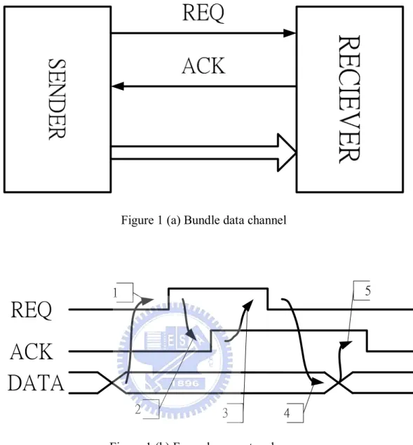
2.1.2 Handshaking Protocols

Handshaking protocols in asynchronous circuit design have two common

methods: one is bundle data protocol (Figure 1 (a)) and the other one is dual-rail

protocol (Figure 2 (a)).

Bundle data protocol has REQ and ACK signals to control all of the transfer

steps, and the most common way is four-phase bundle data protocol (Figure 2 (b)).

Initially, REQ and ACK signals are all 0. When DATA in the SENDER is ready,

REQ signal is pulled up to 1 (1), and then the RECIEVER captures REQ signal and

receives DATA. After receiving DATA, the RECIEVER pulls up ACK signal to 1

(2). At the time the SENDER receives ACK signal, it pulls down REQ signal to 0 (3)

and stops sending DATA, Finally, the RECIEVER pulls down ACK signal to 0 (4)

6

Figure 1 (a) Bundle data channel

REQ

ACK

DATA

Figure 1 (b) Four-phase protocol

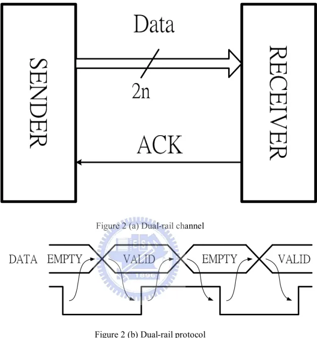
The other way of handshaking is dual-rail protocol. The special place of

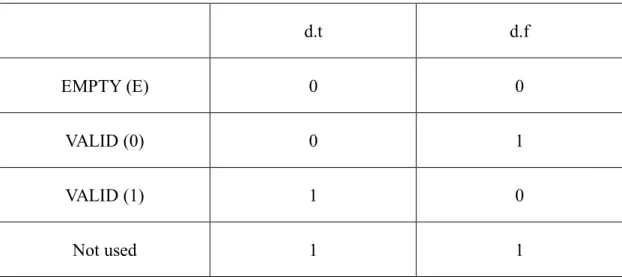
dual-rail protocol is the system does not have REQ signal, and uses 2-bits to encode

1-bit data. The encoding method is shown in Table 1. It uses 00 to shows that there

is no data (EMPTY), uses 01 to encode the data of 0 and 10 to encode the data of 1

(VALID). If the system uses dual-rail protocol to transfer n-bits data, there will be

7 d.t d.f EMPTY (E) 0 0 VALID (0) 0 1 VALID (1) 1 0 Not used 1 1

Table 1 Encoding method

Because of the system does not have REQ signal, the RECEIVER needs extra

circuits to detect DATA signals are arrival. This special design in dual-rail protocol

is called completion detection.

Figure 2 (b) shows the steps if data transfer using dual-rail protocol. Initially,

DATA is EMPTY, and the ACK signal is 0. When DATA is VALID and the

RECIEVER detects that the DATA is ready, the RECIEVER captures DATA and

pulls up ACK signal to 1. And then the SENDER stops sending DATA, so DATA

becomes to EMPTY. Finally, the RECIEVER pulls down ACK signal to 0 and the

8

Figure 2 (a) Dual-rail channel

Figure 2 (b) Dual-rail protocol

VALID will be separated appears. Dual-rail protocol uses EMPTY to separate

each VALID. After the SENDER sends data, the situation will return to EMPTY and

wait for another data. This situation calls return to zero. So the sequence of data is

9

Figure 3 Transfer diagram

Using Dual-rail protocol has another benefit: delay insensitive. This is because

dual-rail protocol encodes the data and has completion detection. The completion

detection lets the circuits without a delay matching, so the circuits are delay

insensitive.

2.2 Interconnection Networks

There are several kinds of interconnection networks, such as sharing bus, net, mesh,

torus system …etc. This paragraph will discuss these ways and compare with them.

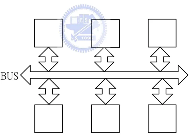
2.2.1 Shared Bus

Shared bus system is the most common way in interconnection networks. All

of the other ways of interconnection networks are the improvement of shared bus

system.

10

Every router on the bus can capture every data, so the routers need to distinguish the

data on the bus. When the router wants to send data, it needs to check the bus is idle,

because the bus only can transfer one data at the same time.

Advantages of the shared bus system:

 It is easy to design the system.

 The cost is lowest.

Disadvantages of the shared bus system:

 The performance is low.

11

2.2.2 Net

Every router in the net system connects to any other routers (Figure 5). The

routers have many inputs and outputs ports. Net system contains maximum data

paths and the most complicated connection.

 The performance is the best.

Disadvantages of the net system:

 The cost is the highest.

 The system is hard to expand.

12

2.2.3 Mesh

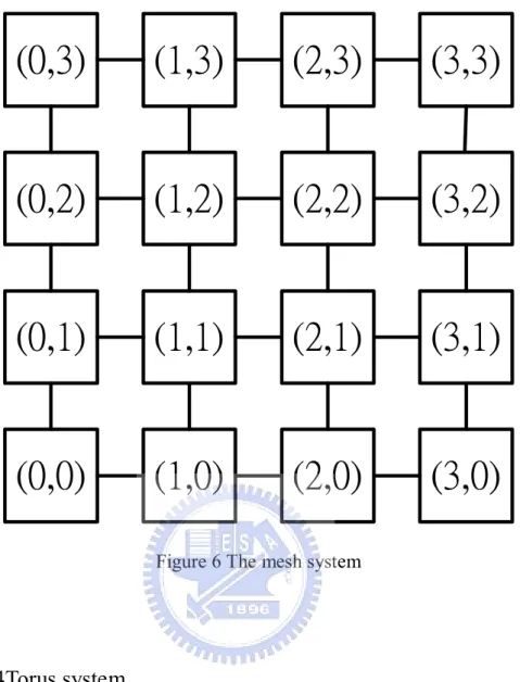
Mesh system can be seen as a two-dimension matrix (Figure 6). Each router in

the mesh system connects to the routers around. The routers in the mesh system can

be separate with three kinds: one is at the corner {(0,0), (3,0), (0,3), (3,3)}, another

one is in the border {(1,0), (2,0), (0,1), (0,2), (1,3), (2,3), (3,1), (3,2)} and the other

one is in the center {(1,1), (2,1), (1,2), (2,2)}. The routers at different places have

different connection ports. Because of the difference, the mesh system needs a

special algorithm to realize transferring data in the system.

Advantage of the mesh system:

 The system arranges in order.

 The cost is lower than the net system.

Disadvantages of the mesh system:

 The critical path is longest.

13

(0,3)

(1,3)

(2,3)

(3,3)

(0,2)

(1,2)

(2,2)

(3,2)

(0,1)

(1,1)

(2,1)

(3,1)

(0,0)

(1,0)

(2,0)

(3,0)

Figure 6 The mesh system

2.2.4 Torus system

The torus system can be seen as an improvement system of the mesh system.

The torus system adds some data paths and modifies the router’s architecture. The

routers on the border connect to the router on the other side of the border. So the

data have a shorter transfer path. The torus system has two different types:

uni-direction torus system (Figure 7 (a)) and bi-direction torus system (Figure 7 (b)).

If the router in the uni-direction torus system, it cannot send data to the router which

14 problem.

Advantages of the torus system:

 The torus system is easy to design. Each router is the same.

 The torus system has a smaller average data path.

(a) (b)

Figure 7 The torus system

2.2.5 Comparison

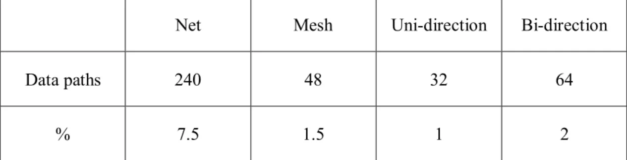
First, we compare with the numbers of the data paths between the

interconnection networks described previously. Suppose that all of the systems have

sixteen routers, and the results are in Table2. The net system has the maximum data

15

bi-direction torus system has sixty-four data paths, and the uni-direction torus

system has the minimum data paths: thirty-two. We can find that the bi-direction

torus system is in among.

Net Mesh Uni-direction Bi-direction

Data paths 240 48 32 64

% 7.5 1.5 1 2

Table 2 The number of data path (16 routers)

The other important issues are the critical data path and the average data paths

in all of the systems. The net system has the smallest critical and average data path:

two, because the routers connect to each other.

The mesh system can be separated into three parts. The critical data path of the

routers at the corner is seven; the critical data path of the routers on the border is six

16

(a) (b) (c)

Figure 8 The data paths of the mesh system

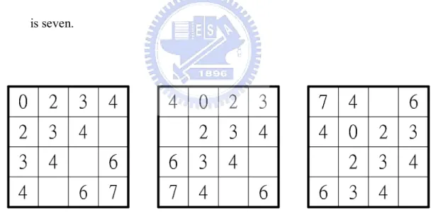
The situations of routers in the uni-direction torus system are shown in Figure

9. All situations of the routers in the system are the same, and the critical data path

is seven.

Figure 9 The data paths of the uni-direction torus system

The situations of the routers in the bi-direction torus system are shown if

Figure 10. Because of the data paths in the system are bi-direction, the critical path

17

Figure 10 The data paths of the bi-direction torus system

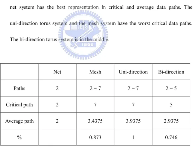
Table 3 shows the comparisons between those interconnection networks. The

net system has the best representation in critical and average data paths. The

uni-direction torus system and the mesh system have the worst critical data paths.

The bi-direction torus system is in the middle.

Net Mesh Uni-direction Bi-direction

Paths 2 2 ~ 7 2 ~ 7 2 ~ 5

Critical path 2 7 7 5

Average path 2 3.4375 3.9375 2.9375

% 0.873 1 0.746

18

2.3 Data Transfer

The popular ways of data transfer in the interconnection networks are wormhole and

packet-switching. Both of them have their advantages and characteristics.

2.3.1 Wormhole

The transformation way of wormhole is to create a channel to transfer data. In

this way, it needs a leading packet that goes first to tell the router where to go.

Behind the leading packet are data packets. The size of the data packets is not fixed.

At last is ending packet and it tells router that the transformation is finished and the

channel can be canceled. Using wormhole to transfer data, the paths are occupied by

one packet sequence at one time, so the rate of router’s exploitation is low.

Furthermore, the wormhole system needs a global controller to check the paths to

avoid the data crash.

For example, if there is a transformation that needs to use Router (0,3),

ROUTER(1,3). The global controller stores the information and let other

transformations do not use them.

2.3.2 Packet-switching

19

packet-switching system are independence and do not influence on other data. Each

packet has its own head to determine the transfer migration. The packets do not

occupy the data paths, so in data-switching system, it allows many packets

transferred at the same time.

For example, if there is a packet that needs to go through Router (0,3),

ROUTER(1,3). The packet use one router at one time and then release the

domination of the router after using.

2.3.3 Deadlock

Deadlock is the most important issue in the transformation system because

deadlock will crash the system. Unfortunately, deadlock would happen in wormhole

system, so the wormhole system needs extra designs such as global controller and

virtual channels [19] to avoid deadlock. But it would not happen in

packet-switching system because the packet-switching system does not occupy data

paths at transformation. Describe in detail, in the packet-switching system, the

packet does not hole the data paths and waits for other data paths and the packets

would not be in the situation of circular waiting. With these two reasons, the

20

2.3.4 Starvation

Starvation is another problem that should be solved. Each outer in our system

has many input and output ports. If one of the packets in the system cannot be sure

to obtain the right of transfer, starvation may happen. To solve this problem, we use

round robin to transfer packets in the system. With round robin, each packets can be

sure that it will be sent.

2.3.5 Comparison

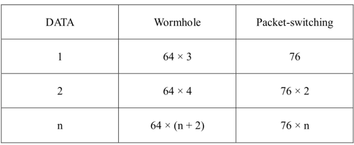
If the system is dual-rail system, the size of data is 32-bits and the head is

6-bits. So the packets in the wormhole system are all 64-bits and the packets in the

packet-switching system are 76-bits. Table 4 shows the sizes of the packets that both

of the systems use.

DATA Wormhole Packet-switching

1 64 × 3 76

2 64 × 4 76 × 2

n 64 × (n + 2) 76 × n

Table 4 The size of packets

21

need to send 192-bits and spend three times to finish the job. But if users use

packet-switching system, they only send 76-bits.

2.4 C-element

C-element is a very important element in the asynchronous circuits. It is usually

used to control the ACK signals and REQ signals. The behavior of C-element is shown

in Table 5. When the inputs are all 0, the output is 0, too. If one of the inputs changes its

status, the output would not change. Until both of the inputs changes to 1, the output

changes to 1. Figure 11 (a) shows the gate level design of C-element. It uses three AND

gate and one OR gate. The output C will connect to the inputs and become one of the

inputs. Figure 11 (b) shows C-element with RESET signal.

a b c

0 0 0

0 1 No change

1 0 No change

1 1 1

22

&

&

&

+

a

b

c

Figure 11 (a) C-element

23

Chapter 3 Design

In chapter 2, we have already compared the advantages and disadvantages of the

asynchronous circuits. In addition, we also describe the benefits of the interconnection

network using the torus system. But there are still some points that can be improved. Chang

propose “Self-timed Torus Interconnection Network with Cut-through Routing Mechanism”

in 2009 [5]. However, because if its circuit routing nature, the network has lots of limitation.

In addition, with its 1-of-5 encoding scheme, it makes it difficult to implement in the real

circuits. Thus, we design a new interconnection network using dual-rail encoding and

packet-switching in the torus system called Asynchronous Bi-direction Interconnection

Network using Torus Topology. This design unifies these two kinds of techniques’ merits, the

asynchronous circuits and the torus system.

This chapter describes with the data flow first, and then it talks about the overall system.

According to these two preconditions, a new algorithm for the routing system and two data

formats to meet the requirements are necessary. The algorithm is the most important part of

our designs, our designs all base on the algorithm. This chapter will describe the router’s

24

3.1 Data Flow

The data flows have two parts: one is used in router and the other is used in

head-building. The first part is shown in Figure 12. This flow shows the data how to

transfer in the router. The router receives the packets from other routers around and

decides that the packet should be kept and sent to the processor or continued transferring

and sent to other routers.

Receive packet from other routers

Arrivial?

Send the packet to the processor

Send the packet to FIFO

FIFO buffer

Send packets out to other routers priority: 1. Y up 2. Y down 3. X left 4. X right

2

1

3

4

5

YES

NO

25

At first, a packet is sent to the router (1). If there are more than one packet arrive at

the same time, the router will receive the packet from up-side first. The priority from

high to low of the four was is up-side, down-side, left-side and right side. Then the router

should determine that the packet is arrival to the destination or not (2). If the packet is

arrival to the destination, the router sends the packet to the processor and the packet has

finished its routing, or else the router sends the packet to the FIFO (3). The packet in the

FIFO waits for the router (4) sending it out to continue routing until the packet arrives to

its destination (5).

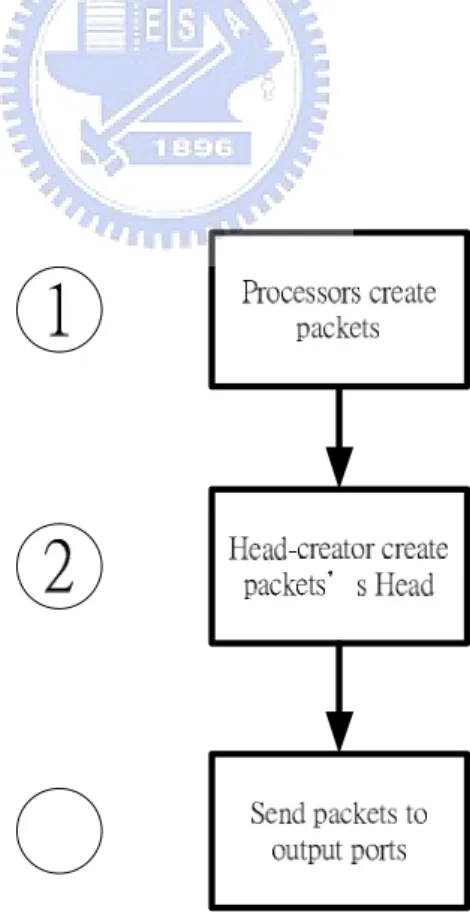
The other data flow shows the data that is created from processors and how to build

its head (Figure 13).

26

Data are created by the processor (1). The only one thing the processor knows is

that the data should be sent to which one of the processor in the system, but the processor

does not know how to transfer the data. So the data are sent to the Head-builder to build

a head and the Head-builder wraps the head in the packet (2). According to the head,

routers can send the packet to the right port and start its routing (3).

3.2 System

The router consists of three major constructions: Arbitrator_One, Arbitrator_Two

and FIFO (Figure 14).

Figure 14 Router’s Architecture

27

packets, Arbitrator_Two is used for sending the packets out and FIFO can be seen as

buffers. Each of the routers has five input ports which can receive the packets from the

neighbor routers and the processor, and they also have five output ports to send the

packets out to the routers around or the processor. FIFO is used to be buffered the input

and the output speed difference. Normally, the input speed is faster than the output speed;

FIFO can let the router receiving the packets continuously, but not stops and waits for the

output.

The routers also need to distinguish the packets between arrival or not. If the packet

is arrival, it will stop routing, or else the packet will continue its travel. This work is

done in Arbitrator_One.

The torus system has two ways to orientate the routers in the system. One is

node-coding [8, 9] and this ways uses a sequence of 0 and 1 to encode each router, like

Johnson code. The routers in the system have their own code. The system which is using

node-coding is hard to expand, because the code should be re-defined when the system

adds new routers. The other way is setting the system like a two-dimension matrix. It

uses X-Y coordinates to orientate each router.

The network system in our design is a bi-direction torus system (Figure 15). We

define the system as a X-Y coordinates. Each row and each column has four routers, so

28

Figure 15 The torus system

Each router in the system has its own identity (ID). The ID is a pair of X-Y

coordinates (X, Y), for example: (0,0), (1,2), (3,2). Thus the router at the low-left is

defined ROUTER(0,0) and the router at the up-right is defined ROUTER(2,2). The

X-coordinates is increasing toward right migration, ex: the right side of ROUTER(0,0) is

29

is on the up side of ROUTER(0,0). Therefore we can easily define the overall system and

use the system.

The routers connect to their neighbor routers and the routers are form beginning to

end connected. The router connects to its neighbor routers means that the router the

router connects to the routers at the up-side, down-side, left-side and right-side. For

example, ROUTER(1,1) connects to ROUTER(0,1), ROUTER(1,0), ROUTER(1,1) and

ROUTER(1,2). The routers connect from beginning to end means that the router on the

border connects to the router on the other side of the border. For example, ROUTER(0,0)

can send a packet to ROUTER(3,0) directly. According to the design, the torus system in

our design has sixty-four connection paths.

Each packet in our torus system has one and only one routing path. The routing path

is decides when the data sent to the router at the first time. So the packet’s routing would

accord with the instruction migration and the packet would not lose its way and be

missed.

Example 1: If ROUTER(2,2) wants to send a packet to ROUTER(0,0), the packet

will go through ROUTER(3,2), ROUTER(0,2), ROUTER(0,1) and ROUTER(0,0) in

30

Figure 16 Transfer orders 1

Example 2: If ROUTER(3,3) wants to send a packet to ROUTER(0,0), the packet

will go through ROUTER(0,3) and ROUTER(0,0) in order (Figure 17).

31

Data transferred in our torus system is using packet-switching. Every packets has its

own head and every packets is the respective independence in the system.

3.3 Routing Algorithms

Routing algorithm can be separated into three parts. The first part handles the

packets which just arrived to the router and the algorithm works in Arbitrator_One. The

second part deals with the packets that are sent out the routers. The third part is used to

build the header for the packets which are sent b the processors, and the algorithm works

in Arbitrator_Two.

3.3.1 Algorithm 1: Arrival

Figure 18 Algorithm 1: Arrival

Algorithm 1 is used to make sure the packet is arrival. This is the most

32

Compare (X_coordinates, X_local) uses OR of XOR to check that is the packet

already at the right column and the result will be stored in Temp_X. If the packet is

at the right column the value of Temp_X is 0, or else the value is 1. Compare

(Y_coordinates, Y_local) uses the same way to check is the packet at the right row

and it stores the result in Temp_Y. According to the values of Temp_X and Temp_Y,

Arbitrator_one can easily know the packet is arrival or not and make right decision

that send the packet to the right place (the processor or the FIFO).

Example 1: Local is (2,2) and the input packet is (2,0). Compare

(X_coordinates, X_local) is compare (2,2), the numbers are the same, so Temp_X

will be 0. Compare (Y_coordinates, Y_local) is compare (2,0), the numbers are not

equal, so Temp_Y is 1. According to Temp_X and Temp_Y, the packet will be sent

to FIFO.

Example 2: Local is (1,1) and the input packet is (1,1). Compare

(X_coordinates, X_local) is compare (1,1), the numbers are the same, so Temp_X

will be 0. Compare (Y_coordinates, Y_local) is compare (1,1), the numbers are the

same, so Temp_Y is 1. According to Temp_X and Temp_Y, the packet will be sent

33

3.3.2 Algorithm 2: Direct-decision

Figure 19 Algorithm 2: Direct-decision

Algorithm 2 is used to determine the packet should be sent to which one of the

output ports. It influence on the packets’ routing paths (Figure19).

Compare (X_coordinates, X_local) uses OR of XOR to check that is the packet

already at the right column and the result will be stored in Temp_X. If the packet is

at the right column the value of Temp_X is 0, or else the value is 1. Compare

(Y_coordinates, Y_local) uses the same way to check is the packet at the right row

and it stores the result in Temp_Y. This part is the same with the front discussion.

But in this algorithm, DECISION also needs X_direct and direct to make right

decision. X_direct and Y_direct store the packet’s travel direction. X_direct and

Y_direct are made by Algorithm 3.

34

Compare (X_coordinates, X_local) is compare (1,2), the numbers are not equal, so

Temp_X is 1. Compare (Y_coordinates, Y_local) is compare (1,2), the numbers are

not equal, so Temp_Y is 1. Because of the value of Temp_X is 1 and the value of

X_direct is 01, DECISION will be 00.

Example 2: Local is (1,1), the packet is (1,0), X_direct is 01 and Y_direct is 10.

Compare (X_coordinates, X_local) is compare (1,1), the numbers are equal, so

Temp_X is 0. Compare (Y_coordinates, Y_local) is compare (1,0), the numbers are

not equal, so Temp_Y is 1. Because of the value of Temp_Y is 1 and the value of

Y_direct is 10, DECISION will be 11.

3.3.3 Algorithm 3: Head-Building

Figure 20 Algorithm 3: Head-Building

35

head-builder and the head-builder is in Arbitrator_two. This algorithm can

determine the packet’s transfer directions (Figure 20).

The routers transfer the packets in compliance with X_direct and Y_direct.

X_coordinates – X_local can let the router knows that the destination is on the right

side or the left side. If the value of X is 1, 2 or -3, it means the destination is on the

right side and the packet will be quite quick by the right side transmission. If the

value of X is -1, -2 or 3, the packet will be quite quick by the left side transmission.

This rule can use in Y. if the value of Y is 1, 2 or -3, the packet should be sent to the

upper-side router and the value of Y is -1, -2 or 3, the packet should be sent to the

under-side router. So the value of X_direct is 01 means the packet goes to right, 10

means goes to left. The value of Y_direct is 01 means the packet goes to up, 10

means goes to down (Figure 21, Table 6).

X-direct Y-direct

0, -1, -2, 3 10 10

1, 2, -3 01 01

36

Figure 21 Signal of transfer direction

Example 1: Local is (1,1) and the packet is (2,2). X_coordinates – X_local is

1 – 2, so the value of X is -1. Looking up the table, the value of X_direct is 10.

Y_coordinates – Y_local is 1 – 2, so the value of Y is -1. Looking up the table, the

value of Y_direct is 10. According to the X_direct and Y_direct, this packet will go

to up-left.

Example 2: Local is (2,2) and the packet is (0,1). X_coordinates – X_local is 2

- 0, so the value of X is 2. Looking up the table, the value of X_direct is 01.

Y_coordinates – Y_local is 2 – 1, so the value of Y is 1. Looking up the table, the

value of Y_direct is 01. According to the X_direct and Y_direct, this packet will go

37

3.4 Packet Sequence

According to the algorithm, each packet has only one routing path, and if the

packets are sent to the same location, the paths are the same, too. So the packets in the

system do not have the packet sequence problem. It means that the packet which is sent

to the destination earlier, it will arrive to the destination earlier than other packets.

3.5 Router

This paragraph describes that how we design the router. First, we design two kind of

packet formats and then we design the overall router.

3.5.1 Packet Formats

The packets in the design have two kinds of formats: one is the processor send

to the router (Figure 22 (a)) and the other one is routers send to each other (Figure

22 (b)).

Each of the formats has two parts: a length of 8-bits or 12-bits head and a

length of 64-bits data. Both of them are using dual-rail encoding, so the real size of

transfer data is 32-bits. The first format which is used in PROCESSOR to ROUTER

has an 8-bits long head and the head only contains destination coordinates(X-Y)

where the packet should be sent to (Figure 23 (a)). The other format is used in

38

destination coordinates but also sending directions (Figure 23 (b)). The sending

directions tell the router that the packet should be sent to which way and the

sending directions are built by the Head-creator. It will be described in the next

paragraph (Head-creator).

(a) Data Format

Figure 22 (b) Data Format

(a) HEAD

39

3.5.2

Head-builder (Figure 24) has two input ports: location and packet_in and one

output port: packet_out. The location is the router’s identity in the Torus system ((X,

Y)), and the length of the location is 4-bits. It is used to check that which direction

the packet should be sent to. The routing algorithm is described in previous

paragraph (Routing Algorithm). Packet_in and packet_out are the data

transformation ports.

Figure 24 Head-builder

Initially, head-creator receives the location and stores it. Then, the processor

sends a packet to the head-builder; the head-builder starts to compare the packet’s

head with location and builds a new HEAD for the packet. The way of the

head-builder determines the packet’s direction is using subtraction (Algorithm 3).

40

new head and data. Finally, Head-builder sends the new packet out. Figure 25

shows the gate-level design of the Head-builder.

M U X M U X

M

er

ge

Figure 25 The detail design of Head-Builder

3.5.3 Arbitrator_One

Arbitrator_one (Figure 26) is used to receive the packet form the routers

around and check out. It has four input ports: four routers around and two output

41 COMPARE_1 BUFFER PROCESSOR Y down Y up X right X left Figure 26 Arbitrator_One

MUX_ONE is used to receive packets and send ACK signal to the senders.

The MUX_ONE can receive one packet at one time. If many packets arrive to the

router at the same time, the MUX_ONE will decide that which one should be dealt

with first. In our design, we use round robin to decide that which one of the packets

can be received and avoid starvation. Based on the design, each packet from routers

around has the same priority, because the SCANNER scans the four ports.

Starvation is a big problem in the interconnection networks. If starvation is

happened, the system will be crashed.

The detail design of the MUX_ONE is shown below (Figure 27). The detects

42

detection is 1, or else the value of detection is 0. ACK_OUT signal tells the sender

that it can stop sending the packet. ACK signal is used to let the REGISTER to

capture the packet.

Figure 27 MUX_ONE

When the packet is received from the MUX_ONE, it will be sent to the

REGISTER. Because the COMPARE_1 stores the location of the router, the

COMPARE_1 can easily make a right judgment that where the packet in the

43

gates. If {packet [73], packet [71], packet [67], packet [65]} is equals to location

[3:0], the value of COMPARE is 0, or the value of COMPARE is 1. The value of

COMPARE decides the packet will go to the PROCESSOR or the FIFO. When the

packet is sent out, the RESET resets the REGISTER, and the REGISTER will wait

for another packet (Figure 28).

R

E

G

IS

T

E

R

44

Figure 28 REGISTER and COMPARE_1

By way of COMPARE_1’s judgment, the packet will be sent to PROCESSOR

or to FIFO by DEMUX (Figure 29). This part also receives the ACK_in signal form

the FIFO and the PROCESSOR, and uses an OR gate to merge these two signals.

D

E

M

U

X

45

3.5.4 Arbitrator_Two

Arbitrator_two (Figure 30) is used to re-packing packets from the processor

and to let the packets go to right routers. It has two input ports: from FIFO and the

processor, four output ports: four routers around.

M

U

X

R

E

G

IS

T

E

R

D

E

C

IS

IO

N

Head-builder has been shown in previous paragraph. It is used to build a new

head for the packets.

MUX (Figure 31) handles that packets from FIFO and Head-builder arrive at

the same time. The design in the Arbitrator_Two is the same with the design in the

Arbitrator_One, we use round robin to make decision. This design can avoid

46

ACK_out

SCANNER

DELAY

MUX

detect_FIFO

detect_processor

packet

Figure 31 MUX in Detail

After receiving the packet from the FIFO or the PROCESSOR, the packet will

be sent to the REGISTER and waiting for the COMPARE signal. The COMPARE

signal can determine the packet should be sent to which output ports. The location

[3:2] subtracts {packet[73], packet[71]} and the location[1:0] subtracts {packet[67],

packet[65]}. The answer of the subtractions will decide COMPARE signal (Table 7).

47 Y = 0 Y ≠ 0, Y_direct = 01 Y ≠ 0, Y_direct = 10 X_direct = 01 00 10 11 X_direct = 10 01 10 11

Table 7 COMPARE signals

D

E

C

IS

IO

N

DECISION is used to send the packet to routers around and receive the ACK

signals. It receives COMPARE signal and sends the packet out (Figure 33).

48

After passing the head-builder, the new head is 0110_1001_1010. According to the

new head, the COMPARE signal is 11; so the packet will be sent to the up-side.

D

E

M

U

X

3.5.5 FIFO

FIFO (Figure 34) in the design can be regarding as buffers. The main utility

solves Arbitrator_one and Arbitrator_two speed different problem. In the design

Arbitrator_two is slower than Arbitrator_one. Arbitrator_two not only receives and

49

check the packets arriving to the destination or not. So Arbitrator_two needs more

time to finish its works.

R

E

G

IS

T

E

R

R

E

G

IS

T

E

R

R

E

G

IS

T

E

R

R

E

G

IS

T

E

R

R

E

G

IS

T

E

R

In the design, FIFO has five stages. According to Muller pipeline, FIFO will be

half-full. So FIFO can pack at most three packets

The deep of FIFO is another important issue. Using five stages is considered at

the same time may receive four packets. One packet stays in Arbitrator_one and

three packets can stay in FIFO.

Figure 35 shows the detail design of the REGISTER.

Because of the multi-inputs C-element is hard to design and it will waste lots of

50

c

c

c

c

c

+

+

data1.t

data1.f

datan.t

datan.f

ACK

data1.t

data1.f

datan.t

datan.f

ACK_out

51

52

Chapter 4 Simulation

In chapter 3, we describe the designs of the function blocks in detail. We use Verilog

HDL to build all of the designs and construct the whole system with above mentioned our

sub-modules in chapter 3.

We implement our asynchronous interconnection network using torus system in

gate-level. The design was synthesized and simulation with the TSMC 130nm library and the

simulator is ModelSim 6.0. The experimental group of our design is the bi-direction torus

system, and the control group is the uni-direction torus system.

4.1 Time Simulation

To make sure our design is correct; we simulate three parts of the main design first.

After confirming the three main parts, we start to test the whole system.

The first simulation is the part of Arbitrator1. Figure 37 shows the simulation of sending

packet to the FIFO. It takes 19174ps to finish this works. Another simulation of the

Arbitrator1 is the packet sent to the processor. We can find that it needs 11392ps (Figure

53

Figure 37 To the FIFO

Figure 38 To the Processor

The second part is the FIFO. Because of the FIFO is combined with many

C-elements, it takes lots of time to pass through one packet. Figure 39 shows the

simulation result. From input to output, it takes 6616ps. In detail simulation, BUFFER0

needs 1996ps, BUFFER1 needs 2197ps, BUFFER2 needs 1250ps, BUFFER3 needs

54

Figure 39 FIFO

The third part is Arbitrator2. The Arbitrator2 receives packets from the FIFO and

the processor. Figure 40 shows the simulation that FIFO sends packets to the Arbitrators

and Figure 41 shows the other simulation. It takes 12090ps to finish transferring the

packet from the FIFO and 13420ps to finish transferring the packet from the processor.

55

Figure 41 From processor

After the testing of the three main parts, we start to simulate the time that sending

packets from ROUTER to ROUTER. The start router is ROUTER(0,3), it sends one

packet to other routers in the system. The simulation is shown in Table 8. The time that

goes through two routers is 24823 ~ 24830ps, the time that goes through tree routers is

64360 ~ 64365ps, the time that goes through four routers is 103907 ~ 103910ps and the

time that goes through five routers is 143445ps. The average time of the simulation is

69636.2ps.

0ps 24823ps 64360ps 24825ps

24820ps 64361ps 103907ps 64365ps

64361ps 103905ps 143445ps 103910ps

24826ps 64360ps 103910ps 64365ps

56

In the previous paragraph, we simulate the bi-direction torus system. Now we

simulate the uni-direction torus system. In the same situation, the total routing time of

ROUTER(0,3) sends packets to other routers is shown in Table 9. The average time is

110543.3pa.

0ps 24523ps 63859ps 103410ps

24520ps 63865ps 103400ps 143446ps

63850ps 103905ps 142950ps 172495ps

103400ps 142945ps 182510ps 217570ps

Table 9 Time simulation of uni-direction torus system

4.2 Area Simulation

The areas of each sub-modules are shown in Table 10, and the areas only contains

whole of the router without the processors. As we can see the area of the FIFO is the

largest. This is because that the sub-module of the FIFO is made up by lots of

C-elements. Each of the C-element contains four gates (three AND gates and one OR

gate). The area of Arbitrator1 is 4566μm2, the area of the FIFO is 15796μm2 and the area

57 module Area (μm2) Arbitrator1 4566 FIFO 15796 Arbitrator2 3849.7 Total 24211.7

Table 10 Area Simulation of bi-direction torus router

The area of the uni-direction torus router is shown in Table 11. The total area of one

router is 22726.4μm2. module Area (μm2) Arbitrator1 3975 FIFO 15796 Arbitrator2 2955.1 Total 22726.4

Table 11 Area Simulation of uni-direction torus route

4.3 Comparison

58

size of uni-direction torus router, and the average routing time of bi-direction torus

system is 58% faster than uni-direction torus system. So we spend 6% extra area to gain

59

Chapter 5 Conclusion and Future Works

In this paper, we design and implement an interconnection network using torus topology.

Our system uses packet-switching routing and bi-direction torus system with new algorithms

to improve the performance of the routing system, avoid the deadlock and starvation.

Moreover we use asynchronous circuits design to solve the problem of global clock and the

system can easily to merge different processors with frequency. Therefore the design can use

in all kind of NOC system.

There are some important reasons using torus system to implement the interconnection

network. First, torus system is easy to design and the routers in the system are all the same. If

the system needs to increase routers, it does not need to change the architecture of the routers.

Second, the torus system has a better performance than mesh system, and the difference of

costs between them are small.

But there still have some points that can be improvement. We use a lot of c-element to

implement the FIFO, so the area of FIFO is very large. Maybe we can use registers to take

place of the c-element and the area may have a better result. The other problem is the deep of

the FIFO. In the design, the deep of the FIFO is five. We do not consider too much, but after

the simulation, we find that the deep of the FIFO can be decreased. The system transfers the

60 performance.

Another place can be improve is the routing algorithms. The algorithm in our design

determines only one routing path for each packet. If there is one router broken, the packets

would not change their routing paths. A good algorithm and router can avoid this situation.

The most popular way of interconnection networks on NOC in recent year is net system.

Because of the number of processors are small, the paths are not too large to place and route.

The torus system has benefits if the system has more than sixteen routers. In this situation,

torus system can balance the cost and the performance.

Finally, our torus system, the results of the simulations: the area of the ROUTER is

61

References

[1] Jens Sparso and Steve Furber, “Principles of Asynchronous Circuit Design“, London, 2001

[2] Lasse Natvig, “High-level Architectural Simulation of the Torus Routing Chip”, pp. 48-55,

IEEE International Verilog HDL Conference, 1997

[3] David Duarte, Vijaykrishman Narayanan and Mary Jane Irwin, “Impact of Technology

Scaling in the Clock System Power”, IEEE International Computer Society Annual

Symposium on VLSI, 2002

[4] R. Y. Chen, M. Vijaykrishma and M. J. Irwin, “Clock Power Issues in System-on-a-Chip

Designs”, 1999, IEEE International

[5] Yuan-Teng Chang, Man-Chen Huang, Wei-Min Cheng, Hung-Yue Tsai, Chang-Jiu Chen,

Fu-Chiung Cheng and Yuan-Hua Chu, “Self-Timed Torus Network with 1-of-5 Encoding”,

pp.569-572, ISCE2009

[6] Angelo Kuti Lusala, Philippe Manet, Bertrand Rousseau and Jean-Didier Legat, “NOC

Implementation in FPGA using Torus Topology”, IEEE International, 2007

[7] Bradley R. Quinton, Mark R. Greenstreet and Steven J. E. Wilton, “Practical

Asynchronous Interconnect Network Design”, IEEE transactions on VLSI System, 2008

[8] Xiaoqiang Yang, Huimin Du and Jungang Han, “Research on Node Coding and Routing

62

[9] Xiaoqiang Yang, Huimin Du and Jungang Han, “A Node Coding and the Improved

Routing Algorithm in Torus Topology”, pp. 443-447, 2008 ICSIT

[10] Donald F. Wann and Mark A. Franklin, “Asynchronous and Clocked Control Structures

for VLSI Based Interconnection Network”, IEEE Transactions on Computer, vol.32 No.3,

March 1983, pp. 284-293

[11] Aydin O. Balkan, Gang Qu and Uzi Vishkin, “Arbitrate-and-Move Primitives for High

Throughput On-Chip Interconnection Networks”, 2004 ISCAS

[12] Paul E. Gronwski, William J. Bowhill, Ronald P. Preston, Michael K. Gowan and Randy

L. Allmon, ”High-Performance Microprocessor Design”, IEEE Journal of Solod-state

Circuits, vol.33 No.5, May 1998, pp. 676-686

[13] William J. Dally, “Performance Analysis of k-ary n-cube Interconnection Networks”,

IEEE Transactions on Computer, vol.39 No.6, June 1990, pp. 775-785

[14] Li-Shiuan Peh and William J. Dally, “A Delay Model and Speculative Architecture for

Pipelined Routers”, pp. 255-266, 2001 IEEE

[15] Wladek Olesinski and Pawel Gburzynski, “Asynchronous Deflection with Transient

Buffers”, pp. 338-345, 1998 IEEE

[16] W. J. Dall and C. L. Seitz, “The Torus Routing Chip”, J. of Distributes Computing,

1(3):187-196, 1986

63 Morgan Kaofmann, 2005

[18] W. J. Dally and C. L. Seitz, “Deadlock-Free Message in Multiprocessor Interconnection

Networks”, IEEE Transactions on Computer, vol36 No.5, May 1987, pp. 539-546

[19] Kermani P., Kleinrlck L., “Virtual Cut-Through: a new computer communication