虛擬實境多媒體影音即時互動之研究

國立交通大學

機械工程研究所

碩 士 論 文

虛擬實境多媒體影音即時互動之研究

The Research for Virtual Reality based Audio-Visual

Interactive Multimedia

研 究 生: 曹 明 亮

指導老師: 成 維 華 教授

中華民國九十六年六月

虛擬實境多媒體影音即時互動之研究

The Research for Visual Reality based Audio-Visual Interactive Multimedia

研 究 生: 曹 明 亮 Student: Ming-Liang Tsao 指 導 教 授: 成 維 華 Advisor: Wei-Hua Chieng

國 立 交 通 大 學 機 械 工 程 研 究 所

碩 士 論 文 A Thesis

Submitted to Department of Mechanical Engineering College of Engineering

National Chiao Tung University In Partial Fulfillment if the Requirements

For the Degree of Master of Science In

Mechanical Engineering June 2007

Hsinchu, Taiwan, Republic of China

虛擬實境多媒體影音即時互動之研究

The Research for Virtual Reality

based Audio-Visual Interactive Multimedia

Student : Ming-Liang Tsao Advisor : Dr. Wei-Hua Chieng Department of Mechanical Engineering

National Chiao Tung University

Abstract

This study proposes an audio-visual interactive multimedia based on DirectX programming. The real-time virtual reality takes a sensor as an input device. This system treats the waterfall in summer and furnace in winter as the scene. The fire effects, the tempo of playback and the volume of playback alter with rising or decreasing temperatures. This literature introduces 3D graphics programming, special effects, audio effect system, and so on.

Acknowledgement

I would like to express my deep appreciation to my advisor Prof. Wei-Hua Chieng. Thank for his instruction and concern both in class and in my life during the two years in the research institute.

I also thank my seniors, Chih-Fang Huang, Shang-Bin Lu, and Yung-Cheng Tung. Thanks a lot. Finally, I would like to appreciate my family, who always help me and encourage me all the time. The support andconsideration of my parents are the great significance to me.

Contents 摘要………i Abstract………..ii Acknowledgement………...……….iii Contents……….………iv List of Figures………...………....vi Nomenclatures………...vii CHAPTER 1 INTRODUCTION……….………...1 1.1 Research Orientation………..…….………...……1

1.2 A Brief Overview of DirectX……....……….2

1.3 The Program Flow…….………...……….3

CHAPTER 2 DirectX Graphics….………..……….…..4

2.1 Direct3D Pipeline………5

2.1.1 Vertex Data………...5

2.1.2 Classic Transform and Lighting………...9

2.1.3 Clipping and Viewport Mapping………14

2.1.4 Texturing………16

2.1.5 Fog………19

2.1.6 Alpha, Stencil, Depth Testing………21

2.2 Special Effects……….………..24

2.2.1 Fire Effects………...………..………24

2.2.2 Texture Transformations………...………..27

CHAPTER 3 Audio System………...31

3.1 DirectAudio……….……….………...31

3.2.1 Initializing DirectSound………..………..…….………32

3.2.2 Using Secondary Sound Buffers………36

3.2.3 Altering Volume, Panning, and Frequency Settings………….………..38

3.3 DirectMusic………..………..40

3.3.1 Starting with DirectMusic………..………41

3.3.2 Altering Music………..……..45

3.4 MP3 Playback Effects………...……….49

CHAPTER 4 Input Device………..………..52

4.1 Serial Communication Overview………...………52

4.2 Serial Protocol……….………...54

4.3 Implementation of Serial Port Communication………...………..54

CHAPTER 5 Results and Conclusion………...63

List of Figures

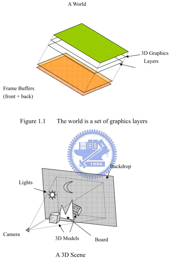
Figure 1.1 The world is a set of graphics layers--- 67

Figure 1.2 The set of the 3D objects in the view--- 67

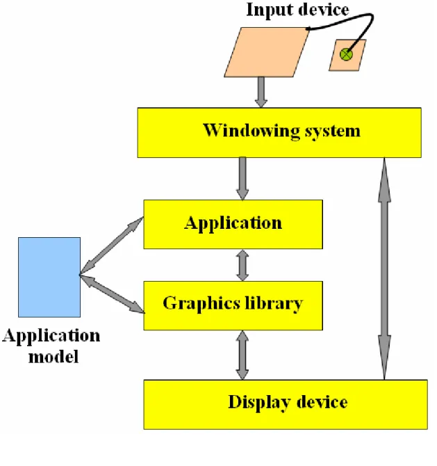
Figure 1.3 System Architecture--- 68

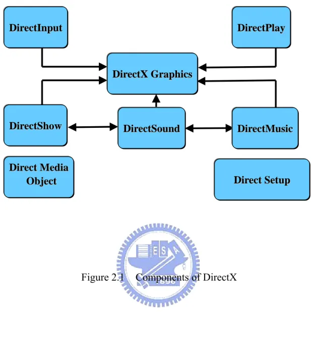
Figure 2.1 Components of DirectX--- 69

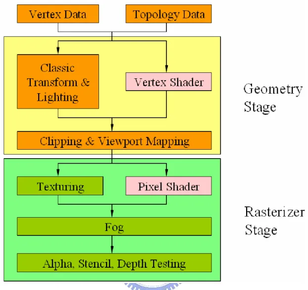
Figure 2.2 Direct3D Pipeline--- 70

Figure 2.3 Vertex Structure in Detail--- 71

Figure 2.4 Primitive Types and Polygons--- 72

Figure 2.5 Sample blend weight functions--- 73

Figure 2.6 Illustration of the effect of blend weight functions--- 73

Figure 2.7 Classic transform of the scene--- 74

Figure 2.8 The effects of lighting and material--- 75

Figure 2.9 Viewport Culling and Clipping--- 76

Figure 2.10 Mipmap--- 77

Figure 2.11 Repeating and Clamping --- 78

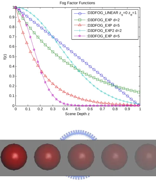
Figure 2.12 Fog factor functions--- 79

Figure 2.13 A case that breaks the Painter’s algorithm--- 80

Figure 2.14 Calculation of z-values--- 80

Figure 2.15 Each fire values--- 81

Figure 2.16 The algorithm for calculating the fire --- 81

Figure 3.1 Flowchart of the sound architecture--- 82

Figure 3.2 MP3 playback flowchart--- 83

Figure 4.1 Serial Communication Protocol--- 84

Figure 4.2 Input device--- 85

Nomenclature

( )

β x = Blend weight function

β = Locating a distance

'

P = The resulting blended vertex position

0 , 1

P P , = A straight line connecting the two transformed points

f C = A fog color C = Object’s color f = A fog factor z = Scene depth e z = RS Fog End s z = RS Fog Start d = RS Fog Density s

α = The alpha value of the source pixel

r

α = The reference alpha values

Chapter 1 Introduction

1.1 Research Orientation

A world is a set of graphics layers where the 3D objects acts on as Figure 1.1 shows. A 3D graphics layer is a projection of the rendering of a 3D view. The set of the 3D objects in the view, we call it the “scene” as Figure 1.2 shows. Computer vision enables us to reconstruct highly naturalistic computer models of 3D environments from camera images. We may need to extract the camera geometry (calibration) scene structure (surface geometry) as well as the visual appearance (color and texture) of the scene. The system architecture is shown in Figure 1.3. We represent the application model which created by 3DS MAX. Then we convert them to x-file format. Above-mentioned concept is very important.

For this literature, we chose two of the most popular special effect techniques used today─fire effect and texture transformations. This system treats the waterfall in summer and furnace in winter as the scene to represent real-time interactive multimedia.

With texture animation, our worlds come alive in ways we can’t imagine. Using everything from basic texture transformations to advanced media playback techniques, we can recreate some awesome effects such as dynamic level backdrops, flowing water, and in─game cinematic sequences. Much like world transformations alter a model’s vertex coordinate data before it is drew, texture transformations alter a model’s texture coordinate data before it is rendered. In other words, we want the appearance of water gushing forth from a waterfall and rolling lazily down a stream.

All science and technology start with the discovery of fire. Of course, to model flames of a real fire accurately is difficult and would require much more CPU power. Like so many other things in game programming, we’re going to produce a fire algorithm that mimics real fire at a fraction of the processing cost. By changing the variables that the fire algorithm uses, we can create a wide variety of fire effects. It looks unbelievably nice.

1.2 A Brief Overview of DirectX

DirectX is a set of low-level application programming interfaces (APIs) for creating games and other high-performance multimedia applications. It includes support for two-dimensional (2D) and three-dimensional (3D) graphics, sound effects and music, input devices, and support for networked applications such as multiplayer games.

DirectX is not a game-creation package; it merely aids in the development of the applications through the use of APIs designed to interface directly with the computer hardware. If the hardware is equipped with DirectX drivers, we have access to the accelerated functions that device provides. If no accelerated functions exit, DirectX will emulate them. This means that we will have a consistent interface with which to work, and we will not have to worry about things such as hardware features. If a feature doesn’t exit on the card, it’s still likely that the feature will work through DirectX’s emulation functions. No fuss, no muss; just program the game and rest assured that it will work on the majority of systems. New versions of DirectX are frequently released, with each new version adding newer features and improving older ones. At the time of this writing, version 9 has been released and that is then version on which this thesis is based.

1.3 The Program Flow

A typical program begins by initializing all systems and data then entering the main loop. The main loop is where the majority of things happen. Depending on the game state that is occurring, we’ll need to process input and output differently. Here are the steps that we follow in a standard game application：

1. Initialize the systems (Windows, graphics, input, sound, and so on). 2. Prepare data (load configuration files).

3. Configure the default state. 4. Start with the main loop.

5. Determine state and process it by grabbing input, processing, and outputting.

6. Return to Step 5 until application terminates and then go to Step 7. 7. Clear up data (release memory resources, and so on).

8. Release the systems (windows, sound, and so on).

Steps 1 through 3 are typical for every game：set up the entire system, load the necessary support files (graphics, sound, and so on).

Chapter 2 DirectX Graphics

Direct3D is a low level graphics API that enables us to render 3D worlds using 3D hardware acceleration. Direct3D can be thought of as a mediator between the application and the graphics device. DirectX is divided into several parts as Figure 2.1 shows.

1. DirectGraphics：This part of DirectX takes care of drawing graphics to the screen. In previous versions of DirectX, there are separate components for 2D graphics (called DirectDraw) and 3D graphics (called Direct3D). With DirectX 9, these components have been combined into DirectGraphics.

2. DirectAudio：This part of DirectX is all about making music and sound effects

3. DirectPlay：This is, in a word, networking. This component allows we to create multiplayer games easily than work over the Internet, modem, LAN, serial line, and so on. It also provides functionality for real-time voice communications in multiplayer games.

4. DirectInput：This provides access to keyboards, mice, joysticks, and other input devices. DirectInput also provides a means to control force feedback devices.

5. DirectShow ： This provides video and multimedia playback capabilities.

We will concentrate mostly on DirectGraphics and DirectAudio in this thesis. Figure 2.2 shows Direct3D pipeline architecture. It is the core of 3D graphics programming. Each major section of the pipeline is treated by a part of this thesis. The application delivers scene data to the pipeline

in the form of geometric primitives. The pipeline processes the geometric primitives through a series of stages that results in pixel displayed on the monitor.

2.1 Direct3D Pipeline

2.1.1 Vertex Data

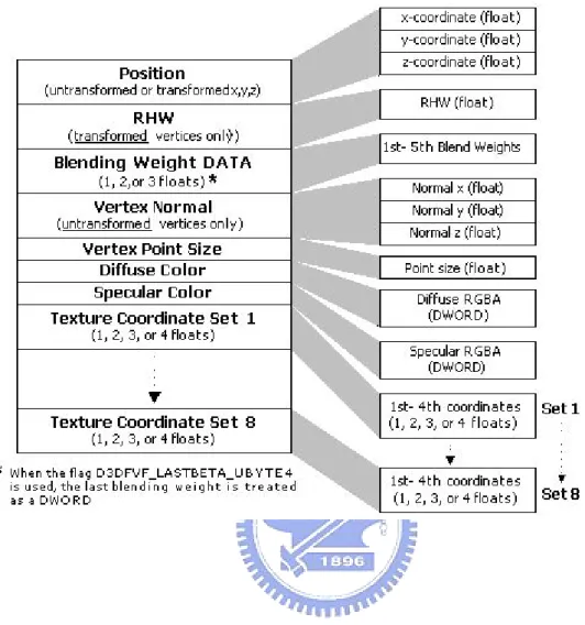
3D models form the foundation of most 3D programs. Simply put, a model is a collection of vertices, with some additional properties for each vertex (the corresponding texture coordinate for that vertex, the vertex’s normal, and the like). We construct everything in the 3D world from vertices. Vertices form triangles, triangles form surface, and surfaces form the hollow models. A programmer that renders a complex 3D world wants to hand Direct3D all sorts of information about a vertex as shown in Figure 2.3, not only its position in world space also its normal, material, color, and the like.

To render the model properly, Direct3D must interpret the vertices we give it and must form those vertices into triangles. It can do this in three ways：Triangle lists, triangle strips, and triangle fans. Direct3D calls these primitive types as Figure 2.4 shows. In a triangle list, each vertex of each triangle is specified. In a triangle strip, the first three vertices define a triangle. Direct3D forms the next triangle by using the last two vertices of the first triangle and one new vertex. Direct3D forms the third triangle using the last two vertices of the second triangle and one new vertex. In essence, every triangle shares two of its vertices with the preceding triangle. In a triangle fan, we send Direct3D the vertex at the base of the fan, followed by all the vertices on the top of the fan, and it’s smart enough to know that the end vertex for one triangle is the start

vertex for another. Essentially, each triangle in the fan has the same base vertex and one vertex it shares with its fan neighbor. In fact, triangle lists are the most widely used.

Direct3D gives us the freedom to define a vertex in many different ways. For example, if we’re using 2D graphics, we can specify coordinates in 2D screen coordinates (transformed coordinates). On the other hand, if we’re using local or world space coordinates, we can specify coordinates in 3D (untransformed coordinates). The flexible vertex format (FVF) is used to construct the custom vertex data for use in the applications. With FVF, we get to decide what information to use for the vertices; information such as the 3D coordinates, 2D coordinates, color, and so on. We construct the FVF using a standard structure in which we add only the components we want. There are some restrictions of course, as we must list the components in a specific order, and certain components cannot conflict with others (such as using 2D and 3D coordinates at the same time). Once the structure is complete, we construct a FVF descriptor, which is a combination of flags that describe the vertex format. The following code bit contains a vertex structure using the various variables allowed with FVF. The variables in the structure are listed in the exact order they should appear in the structures. If we cut any variables, make sure we maintain the order as shown：

typedef struct{

FLOAT x, y, z, rhw; // 2D coordinates FLOAT x, y, x; // 3D coordinates FLOAT nx, ny, nz; // Normals

D3DCOLOR diffuse; // Diffuse Color

FLOAT u, v; // Texture coordinates; } sVertex;

including the normals. Normals are coordinates that define a direction and can be used only in conjunction with 3D coordinates. We need to pick which set of coordinates (2D or 3D) to keep and which to discard. If we are using the 2D coordinates, we cannot include the 3D coordinates, and vice versa. The only real difference between the 2D and 3D coordinates is the addition of the rhw variable, which is the reciprocal of the homogeneous W. This typically represents the distance from the viewport to the vertex along the Z-axis. We can safely set rhw to 1.0 in most cases. In order to describe a FVF descriptor, we combine all the appropriate flags into a definition (assuming the 3D coordinates and diffuse color component)：

#define VertexFVF (D3DFVF_XYZ | D3DFVF_DIFFUSE)

Just make sure that all the flags match the components that we added to the vertex structure, and everything will go smoothly.

After we construct the vertex structure and descriptor, we create an object that contains an array of vertices. Before we can add vertices to the vertex buffer object, we must lock the memory that the buffer uses. This ensures that the vertex storage memory is in an accessible memory area. We then use a memory pointer to access the vertex buffer memory. Here we have the offset into the buffer at the position we want to access (in bytes), as well as the number of bytes we want to access (0 for all). Then all that we need to do is give the function the pointer to the memory pointer that we’re going to use to access the vertex buffer. Now we have the vertex structure, descriptor, and buffer and we are locked and ready to store vertex data. All we need to do is copy the appropriate number of vertices into the vertex buffer. That’s all there is to constructing a vertex buffer and filling it with vertex data.

Another property, the simplest case of vertex blending is when two matrices and a single weight are used to blend between the two transformed points. This formula is similar to the alpha blending formula. Vertex blending with a single weight may be visualized as interpolating along a straight line connecting the two transformed points P0 andP1,

with β_{locating a distance along the line.P}'_{is the resulting blended}

vertex position.

'

0 1

= + (1- )

P βP β P _(2-1)

Assigning a βvalue to each vertex defines the ratio of transformations at each vertex. Usually the blend weight values will be assigned by a modeling program where a user interface is provided for controlling the appearance of vertex blending. There are four blend weight functions

( ) β x _{defined for x in [0, 1].} 25( 0.5) ( ) 1 sin( ) ( ) 1 1 ( ) 1 2 , [0, 0.5] ( ) 2(1 ), (0.5,1] x x x x x x e x x x x x β π β β β − − = − = − = + ∈ ⎧ = ⎨ _{− ∈} ⎩ (2-2)

Figure 2.5 plots four different distributions of blend weights on the interval [0, 1]. Figure 2.6 shows the result of applying a translation using those distributions. The blend weights were computed for the model by normalizing the x coordinate of each vertex into the interval [0, 1] and computing β x( )_.

2.1.2 Classic Transform and Lighting

As Figure 2.7 shows, a typical 3D application has several local coordinate systems (one local coordinate system for each 3D model). The origin of each of those local coordinate systems is usually at the center of that particular 3D model. In addition, a typical 3D application has one world coordinate system, whose origin is literally the center of the game universe. The first order of business is to take all the model’s local coordinates and transform them into world coordinates so that they all share a single world again.

Converting local vertices on a model to world vertices is the same as applying a transformation to them. In the world transformation step, the system multiplies each model’s vertex by a matrix that rotates it, scales it, and translates it to a specific position in the world. Of course, each model has a separate matrix. After we do this for all the models in the scene, there is no longer any notion of model space. The matrix we plug into the assembly line to place the model in the world is called the world transformation matrix. It’s named this because it’s the matrix that transforms local coordinates into world coordinates.

3D hardware simply renders the vertices which means that the viewer of the scene is hard-coded to be at (0, 0, 0), looking down the positive z-axis into the screen. Simply transforming all the model vertices into world vertices isn’t enough. We need to transform them one more time to account for where the viewer of the world is. All it takes is another pass through the vertex-processing assembly line. The camera position is shifted to the world origin (0, 0, 0), and is right side up. This is

the second step in the pipeline. For example, there is a teapot floating in space at position (11, 17, 63). Now imagine that we put a camera at (11, 17, 63), looking in a positive z direction. What we’d expect the camera to see would be an-closed-and-personal image of the teapot. After all, the camera is only one unit in front of the teapot and is looking right as it. Unfortunately, graphics hardware can render scenes only as seen from (0, 0, 0). To deal with this, we just move everything in the world by (-11, -17, -62), which works because now the camera’s at (0, 0, 0) and that makes the graphics hardware happy. The teapot also is moved (-11, -17, -62), so it ends up at position (0, 0, 1), still one unit in front of the camera. In other words, everything is relative. It doesn’t matter where exactly the camera is located. What matters is where it’s located relative to all the other objects in the scene. That’s how cameras work. The view transformation matrix is simply the matrix that takes each vertex and translates it so that the camera is at (0, 0, 0) and facing straight up (positive y-axis). Most view matrices are concatenations of four matrices ： one matrix that translates the objects and three rotation matrices that rotate the world so that the camera’s x, y, and z axes are pointing correctly. That is, positive x-axis pointing left, positive y-axis pointing up, and positive z-axis pointing into the scene.

After we do view transform, we have a set of vertices that graphics programmers consider to be in view space. They’re all set up. The only problem is that they’re still 3D, and the screen is 2D. Projection transformation takes all the 3D coordinates and projects them onto a 2D plane, at which point they’re said to be in project space. It converts the coordinates by using a matrix called the projection transformation matrix. Projection transformation matrix set up the camera’s filed-of-view and viewing frustum.

Next on the list of advanced graphics techniques is the use of lighting. Unlike in real-life, most games fully illuminate the scene, which does make graphics look sharp, albeit unrealistic. To get a more true-to-life scene, and to give the graphics those subtle lighting effect, we need to utilize Direct3D’s lighting capabilities. We can use four types of light in Direct3D：ambient, point, spot, and directional. Ambient light is a constant source of light that illuminates everything in the scene with the same level of light. Because it is part of the device component, ambient light is the only lighting component handled separately from the lighting engine. The other three lights have unique properties. A point light illuminates everything around it (like a light bulb does). Spotlights point in a specific direction and emit a cone-shaped light. Everything inside the cone is illuminated, whereas objects outside the cone care not illuminated. A directional light (a simplified spotlight), merely casts light in a specific direction.

Lights are placed in a scene just as other 3D objects are─by using x, y, z coordinates. Some lights, such as spotlights, also have a direction vector that determines which way they point. Each light has an intensity level, a range, attenuation factors, and color. That’s right, even colored lights are possible with Direct3D. With the exception of the ambient light, each light uses a D3DLIGHT9 data structure to store its unique information. It contains all the information we need in order to describe a light. Although the lights don’t necessarily use every variable in the D3DLIGHT9 structure, all the lights share a few common fields.

Point lights are the easiest lights with which to work. We just set their positions, color components, and ranges. Spotlights work a little differently than the other lights do because spotlights cast light in a cone

shape away from the source. The light is brightest in the center, dimming as it reaches the outer portion of the cone. Nothing outside the cone is illuminated. We define a spotlight by its position, direction, color components, color components, range, falloff, attenuation, and the radius of the inner and outer cone. We don’t have to worry about falloff and attenuation, but need to think both radiuses of the cone. Programmers determine which values to use and we’ll just have to play around until we find the values we like. In terms of processing, directional lights are the fastest type of light that we can use. They illuminate every polygon that faces them. To ready a directional lights for use, we just set the direction and color component fields in the D3DLIGHT9 structure. Ambient lighting is the only type of light that Direct3D handles differently. Direct3D applies the ambient light to all polygons without regard to their angles or to their light source, so no shading occurs. Ambient light is a constant level of light, and like the other types of light, we can color it as we like.

There doesn’t seem to be a limit to the number of lights that we can use in a scene with Direct3D, but keep the number of lights to four or less. Each light that we add to the scene increases the complexity and the time required for rendering.

Materials comprise the second half of the Direct3D lighting system. Direct3D allows us to assign materials to vertices and, therefore, to the surface the vertices create. Each material contains properties that influence the way light interacts with it as Figure 2.8 shows. A Direct3D material is basically a set of four colors：diffuse, ambient, emissive, and specular.

Diffuse color has the most effect on the vertices because it specifies how the material reflects diffuse light in a scene. This parameter tells Direct3D what colors the object reflects when hit with light. In essence, this determines the color of the object under direct light. Say that we set up a model using only material and specify a diffuse color of RBG (255, 0, 0) for that material. This means that the object reflects only red light. When hit with a white light, the object also appears red because the only light it reflects is red light. When hit with a red light, the object also appears red. When hit with a blue or green light, however, the object appears black because there’s no red within the blue or green light to reflect.

The intensity of the reflected light depends on the angle between the light ray and the vertex normal. The intensity is strongest when the light rays are parallel to the vertex’s normal, in other words, when the light is shining directly onto the surface. The intensity is weakest when the light rays are parallel to the surface, because it’s impossible for them to bounce off the surface when they’re parallel to it.

The ambient color property determines a material’s color when no direct light is hitting it. Usually, we set this equal to the diffuse color because the color of most objects is the same when hit by ambient light and when hit by diffuse light. However, we can create some weird-looking materials by specifying an ambient color that’s different from the diffuse color. Ambient color always has the same intensity because it is assumed that the ambient light is coming from all directions.

We use emissive color to create the illusion of materials that glow. They don’t actually glow─Direct3D doesn’t perform lighting calculations using them as a light source─but they can be used in scenes to create the

appearance of a glowing object, without requiring additional light processing. For example, we can create a material that emits a white color and use it to simulate an overhead fluorescent light in the scene. It won’t actually light up anything. We have to compensate for they by, say, assigning a bright ambient color to the objects in the scene.

Last but not least, we use the specular color of a material to make an object shiny. Most of the time, we set the specular color to white to achieve realistic highlights, but we can set it to other colors to create the illusion of colored lights hitting the object. Another property, specular power, goes hand-in-hand with specular color. The power property of a material determines how sharp the highlights on that material appear. A power of zero tells Direct3D than an object has no highlights, and a power of 10 creates very definite highlights.

2.1.3 Clipping and Viewport Mapping

Camera and viewports are different things. A viewport defines the destination of the 3D rendering. Whereas a camera represents a position and orientation in the 3D world we want to render. A viewport defines a destination rectangle into which Direct3D renders the scene. Viewports also allow us to define the range of z-values we want in the final scene. A viewport is a 3D box; it has width, height, and depth. In Direct3D , we specify the viewport’s rectangle using four variables：X, Y, Width, and Height. Direct3D assumes that the X and Y values represent the screen coordinates relative to the top-left corner of the rendering surface and that Width and Height represent the width and height of the viewport. A viewport has two additional variables, MinZ and MaxZ, which tell Direct3D the minimum and maximum z-values of the rendered scene. We will see more precisely how these values come into play on the 3D

geometry pipeline, but for now just realize that most of the time we set MinZ to 0.0 and MaxZ to 1.0. Note that most 3D games fill the entire screen with a 3D scene, so the viewports of most 3D games have x/y values of (0, 0) and width and height values equal to the width and height of the back buffers. We can set MinZ and MaxZ to values other than 0.0 to 1.0 to achieve special effects. For example, if we’re rendering a heads-up display onto a previously rendered scene, we probably want both MinZ and MaxZ to be 0.0, which guarantees that Direct3D will put the scene we’re rendering on top of everything else.

When we refer to a camera in 3D graphics programming, what we’re talking about is ultimately a combination of the view matrix and the projection matrix. The view matrix is like the position and orientation of the camera. The view matrix transforms the world coordinates so that they form a scene as viewed from a certain position and orientation in a 3D space. The projection matrix determines the camera’s field of view, along with the nearest and farthest point a camera can see. The projection matrix takes the 3D points in the 3D world and converts them to 2D points on the screen. In other words, it “projects” the 3D world onto a 2D plane.

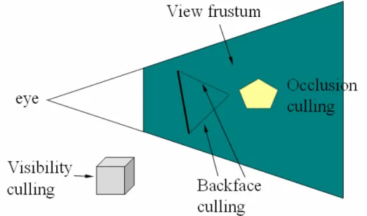
The field of view, along with the near and far clipping planes, defines a view frustum, a pyramid with a flat top instead of a point. The finished 3D scene contains only the objects inside this frustum─all other objects are not visible. Some objects might have to be clipped, if they’re partially inside the frustum as shown Figure 2.9 shows.

Direct3D supports different ways to project the 3D scene onto a rectangular rendering surface. The most common projection is the perspective projection. When we use this projection, Direct3D creates the

illusion of 3D by making objects in the distance appear smaller than objects up close. The second most common projection is an orthogonal projection, in which distant objects are not rendered smaller than near objects. Orthogonal projection don’t scale the size of the objects they render, which makes them useful when we want to stop Direct3D from shrinking far away objects and enlarging near objects. For example, when we’re using Direct3D to write a 2D game, we may still want to use z values to determine the drawing order, but we may not necessarily want the size of the sprite to change.

After the vertices come through projection transformation, Direct3D looks at each one and discards the ones that aren’t visible on the screen. Direct3D might have no do more work than just removing a vertex. If the vertex it removed is part of a surface that is on the screen, Direct3D might have to do some additional work with that vertex so that the surface on-screen appears to have a vertex off-screen. At this point, it also looks at the MinZ and MaxZ values we specified when we set up the viewport, and it scales the z-values of all the vertices so that they fit within the range. After the vertices come through the clipping and viewport mapping process, they’re sent to the rasterizer, which takes the vertex data and begin drawing the pixels of the scene.

2.1.4 Texturing

Direct3D stores textures as surfaces. This means that anything we can get into a surface as a texture. We can load it from a bitmap. Direct3D provides utility functions that allow us to create a texture straight from a BMP file, or generates the pixel data, using a fractal algorithm. This also means that we specify the pixel format we’d like when we’re creating textures, just as we specify a pixel format for the

back buffer. Most of time, we want the textures to be the same format as the back buffer, but in a few scenarios we want them to differ─for example, if we want to save graphics memory by using paletted textures. There’s one important caveat involving texture surfaces. Usually, their width and height must be powers of 2. This means that 2×_{2, 4}×_{4, 8}×_8,

and so on. Textures are okay.

After we load a texture into a memory pool, the next logical step is to tie it to a surface of a 3D model. The way to do is through the model’s vertices. Recall that when we create a flexible vertex format (FVF), one of the properties we can include in the vertex is a texture coordinate. This texture coordinates tells Direct3D what texel should be placed at that vertex. For a 2D textures, this texture coordinate is made up of two components, a u-value and v-value, which correspond to the x-value and y-value in 2D space. This information, combined with the texture coordinates for other vertices, tells Direct3D how the texture fits onto the surface. Direct3D considers the entire width of the texture to be a 1.0 texture coordinate unit wide, and the entire height of the texture to be 1.0 texture coordinate unit tall. In other words, regardless of the texture’s resolution, a (u, v) coordinate of (1.0, 1.0) always represents the lower-right corner, and a (u, v) coordinate of (0.5, 0.5) always represents the center of the texture. Here’s the most common process we go through when using textures：

1. Make sure that the device we’re running on supports the texture operations we need.

2. Load the texture from disk, or if we’re using an algorithm to generate the texture, generate the texels manually.

coordinate that tells Direct3D which texel corresponds to that vertex. 4. In the rendering code, select a texture for a surface, and them pump

the vertices that use this texture into Direct3D. Select a different texture, pump those vertices in, and repeat until everything is textured. Repeat for each frame of the game.

5. Release the texture interface when we’re done with it.

One of the most basic problems to solve when it comes to texturing involves how exact the computer is when taking a bitmap of a certain dimension and mapping it to a surface that’s bigger or smaller. Texturing-filtering modes determine how Direct3D deals with this problem. Direct3D supports several types of texture-filtering modes： linear filtering, mipmap filtering, anisotropic filtering, and no filtering (nearest-point sampling).

Linear filtering is a step up from nearest-point sampling. When using this method, Direct3D calculates a weighted average between the nearest four texels adjacent to the calculated texel. Because the average is weighted, this creates a smooth blending effect. Small textures rendered to big surfaces appear out of focus but less blocky than with nearest-point sampling. Direct3D supports are bilinear filtering. What it means is that several pixel colors are combined to create the final image. Resource-wise, linear texture filtering is a good compromise between nearest-point sampling and mipmap texture filtering. Linear texture filtering requires a medium amount of CPU power.

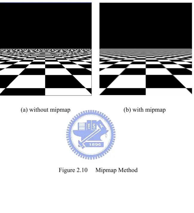
Mipmap texture filtering hogs memory but allows for quick and highly realistic texture rendering. In essence, the technique of mipmapping involves using several bitmaps of varying sizes as one texture. Direct3D uses high-resolution bitmaps for objects close to the

viewer and low-resolution bitmaps for objects far away. This enables us to filter and tweak the low-resolution bitmaps manually so that they become highly accurate counterparts to the high-resolution texture as Figure 2.10 shows. Each bitmap in a mipmap chain must be smaller than the one before it by exactly one power of 2. if the highest-resolution image is 512×_{512, the smaller images must be 256}×_{256, 128}×_{128, and} so on. In addition, we can use mipmapping in conjunction with nearest-point sampling or linear filtering.

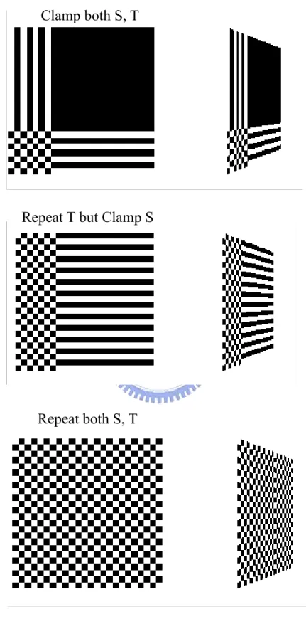
Usually, (u, v) coordinates are between 0.0 and 1.0, but they don’t have to be. The active texture addressing mode tells Direct3D what to do when a (u, v) coordinate falls outside this range. We can choose from four addressing modes as Figure 2.11 shows：wrap, mirror, clamp, and the border color. When the wrap addressing mode is active, Direct3D tiles the texture repeats itself every 1.0 coordinates. Mirror addressing is very similar to wrap addressing in that the texture repeats itself every 1.0 coordinate. The difference is that each tile is a mirror of its adjacent tiles. In clamp addressing, Direct3D does not tile the image. Instead, it treats any u or v coordinate above 1.0 as if it were 1.0, in effect duplicating the last row and column of the texture across any coordinates greater than 1.0.

2.1.5 Fog

Fog, also called depth-cueuing, is an effect that changes an object’s color based on its depth from the camera. The object’s color C is changed by blending it with the fog color Cf using a fog factor f .

' _{= + (1- )}

f

The fog factor f _{is computed based on the object’s distance from the}

camera. Fog changes the color of objects, but it does not change an object’s transparency, so the alpha channel remains untouched by the fog blend. Direct3D provides support for two kinds of fog applications： vertex fog and pixel fog, only one of these can be used at a time and pixel fog cannot be used with programmable vertex shaders. With vertex fog, the fog factors are computed per-vertex as part of vertex processing and these fog factors are interpolated for each pixel produced by rasterization. With pixel fog, also called table fog, the fog factors are computed per-pixel during rasterization, usually by a table lookup from the pixel’s depth. Direct3D also allows an application to compute the fog factor for each vertex and supply it to the rasterizer for interpolation. Once the fog has been determined, the fog blend is applied to the pixel as the last stage of pixel processing.

RS Fog Enable controls the application of fog altogether. If this state is FALSE, then no fog computations are performed. The fog color Cf is

defined by RS Fog Color; only the RGB channels are used. With fixed-function processing, one or both of RS Fog Mode and RS Fog Vertex Mode can be set to D3DFOG_NONE. To supply application computed fog factors, either through stream data or a programmable vertex shader, set both fog modes to D3DFOG_NONE and RS Fog Enable to TRUE. The fog mode selects a formula that is used to compute the fog factor based on depth. The formulas are plotted in Figure 2.12 and give below.

2 ( ) 1, 3 _ ( ) , [ , ] 0, 3 _ ( ) 3 _ 2 ( ) s e s e e s e dz dz z z z z D DFOG LINEAR f z z z z z z z z D DFOG EXP f z e D DFOG EXP f z e − − ⎧ < ⎪ ₋ ⎪ =_⎨ ∈ − ⎪ ⎪ _> ⎩ = = (2-4)

Linear fog ramps from the object’s color to the fog color when the depth is in the range [ , ]z z_{s e . Exponential fog makes a smoother}

transition between the object’s color and the fog color. Exponential fog has a density parameter d that controls the falloff of the fog factor. The fog distance is usually computed as the distance to a plane at depth z from the camera. For points distant from the center of the image, this is not the true distance between the camera and the point. Range-based fog computes the true distance from a point to the camera for use with the fog factor formula.

2.1.6 Alpha, Stencil, Depth Testing

After the fog color has been applied to source pixels, they can be subjected to a rejection test based on the transparency (alpha) value of the source pixel. If the alpha test is enabled, a comparison is made between the alpha value of the source pixel and a fixed alpha value given by a render state. If the test fails, the pixel is discarded and no further processing is performed on the source pixel. We can reject completely transparent pixels which have no effect on the final rendering. This eliminates work in the frame buffer and can increase the rendering throughput when a significant number of pixels are likely to be completely transparent. This is often the case when a texture is used as a cutout for a shape, with a large number of completely transparent pixels in the texture. The alpha test comparison is given by the equation.

s r

α op α _(2-5)

Be careful not to confuse to the alpha test, which rejects source pixels based on their alpha value, with alpha blending, which uses the alpha of the source pixel to combine the source pixel with the frame buffer. The alpha value in the interval [0, 255], where 0 corresponds to fully-transparent and 255 corresponds to fully-opaque.

The stencil buffer is used in conjunction with the Z buffer. The stencil buffer can provide arbitrary rejection of source pixels based on the results of the depth test combined with the result of the stencil test. The stencil test compares the value of the current stencil reference value with the stencil buffer value at the destination pixel location. New values computed for the stencil buffer itself are computed according to one of three possible cases for a source pixel.

1. The stencil test failed.

2. The stencil test passed and the depth test failed. 3. The stencil test passed and the depth test passed.

The render states RS Stencil Fail, RS Stencil Z Fail, and RS Stencil Pass, respectively, define the operation performed on the existing stencil buffer value to compute a source stencil value for each of the three cases. The values for these render states are given by the D3DSTENCILOP enumerated type.

There’s a still one important concept：depth buffers. Depth buffers are a crucial element of 3D programming. One of the most difficult aspects of rendering a 3D scene is determining which polygons are covered up by other polygons closer to the viewer. Throughout the years,

many algorithms have been created to address this problem. For example, the Painter’s algorithm says, ”Start at the back, and draw everything in order from farthest away to closest.” In other words, this means rendering the scene as a painter would paint a picture, by first drawing the objects in the background and then drawing over it with the objects in the foreground. At first thought, this sound like a great solutions, but consider the infamous case of three overlapping polygons as Figure 2.13 shows. In this scenario, all the polygons overlap each other to some extent, so no matter which polygon the system chooses to render first, the scene will be incorrect. As we see, to render this scene properly, we can’t simply decide which vertex is closer to the viewer. Depth buffers allow us to occlude things on a per-pixel level.

As shown in Figure 2.14, a depth buffer is a 2D array of numbers that has the same dimensions as the final scene. If rendering a 640*480 image, the depth buffer must be 640*480. the 3D graphics hardware stores the depth buffer in its RAM. When we first start a scene, we clear the depth buffer by setting every array element to its highest possible value. Then, for each pixel we want to render, we compare the pixel’s z-value to the corresponding number in the depth buffer. If the pixel’s z-value is lower than the number in the depth buffer, we plot the pixel and store its z-value in the depth buffer. If the pixel’s z-value is greater than the number in the depth buffer, we don’t render the pixel. Essentially, as we render the scene, the depth buffer keeps tracks of the lowest z-value. The only way we can put a pixel on the screen (and overwrite what’s there already) is by having a z-value lower than the current lowest z-value for that point. That’s how a depth buffer works.

2.2 Special effects

2.2.1 Fire Effects

In essence, the fire algorithm is nothing more than a blend function which combined with careful use of color and clever dampening functions. The fire is just an array of fire values. Each fire value determines how hot the fire is at that particular point as shown as Figure 2.15.

Each pixel of the fire is 1 byte; 0 means as cold as possible, and 255 means as hot as possible. These fire values are mapped to an appropriate color by using a 255-color palette. For example, we’d probably choose to map fire value 255 to RGB (255, 255, 255) and fire values 0 to (0, 0, 0), with red, yellow, and blue colors for the fire values in between. We use these fire values to put texels on a fire texture. We then use the fire texture to texture the objects on which we want the flames to appear.

Every frame, we process the entire fire array. For each fire value in the array, we do the following (See Figure 2.16)：

1. Get the fire values immediately above and below and to the left and right of the fire value we’re processing. For fire values on the edge of the fire array, we can wrap around, or say that their neighbors are 0. 2. Add all four of these values, and then divide that sum by 4.

3. Subtract an amount, usually a small amount, from the calculation. This emulates the fire flames cooling.

That blends the pixels together, but one piece is still missing─we need to get the flames burning upwards. To do this, we take all the new fire values and move them up by 1 so that a calculation for the fire values at (x, y) is stored at (x, y-1) in the fire array. Note that because we have to move the new fire values, we can’t use just one fire array. To process a frame of fire, we need two arrays：one array describing the fire array currently and a blank array “scratchpad” into which we can put the calculations. When we’re done with all the calculations, we use the filled-up scratchpad array to color the texels of the fire texture. We determine the color of each texel by looking at the corresponding fire value and using that as an index into the fire color palette. Finally, after we’re done with one frame, we swap buffers so that the new calculations become current and the old array becomes a scratchpad for the next frame. We also need to fuel the fire by adding random amounts to each fire on the bottom row. That is how we create a fire effect. The fire algorithmic code is given below：

void ProcessFire(unsigned char* firefield, unsigned char* firefield2, int firesizex, int firesizey, int coolamount)

{

for(int y=0; y< firesizey; y++) {

for(int x=0; x< firesizex-0; x++) {

unsigned char firevalue_left, firevalue_right, firevalue_bottom, firevalue_top; int finalfirevalue;

int xplus1, xminus1, yplus1, yminus1;

xplus1 = x+1; if(xplus1 >= firesizex) xplus1=0; xminus1 = x-1; if(xminus1 <0) xminus1 = firesizex - 1;

yplus1 = y+1;

if(yplus1 >= firesizey) yplus1 = firesizey - 1; yminus1 = y-1; if(yminus1 <0) yminus1 = 0;

firevalue_right = firefield[ (y*firesizex) + xplus1 ]; firevalue_left = firefield[ (y*firesizex) + xminus1 ]; firevalue_bottom = firefield[ ((yplus1)*firesizex) + x ]; firevalue_top = firefield[ ((yminus1)*firesizex) + x ]; finalfirevalue = (firevalue_left + firevalue_right + firevalue_top + firevalue_bottom)/4;

finalfirevalue -= coolamount;

if( finalfirevalue < 0 ) finalfirevalue = 0;

firefield2[ ((yminus1)*firesizex)+x ] = finalfirevalue; }

}

// just pick one and stay with it around with the code to get //various by changing the below code to various parts gives //different effects.

// Add fuel to the fire value on the scratch array. for(int x=0; x< firesizex; x+=2)

{

int y=firesizey-1;

int fuel = firefield[ (y*firesizex) + x ] + (rand() % 64) - 32;

if( fuel > 255 ) fuel = 255; if( fuel < 0 ) fuel = 0;

firefield2[ (y*firesizex) + x ] = (unsigned char)fuel; firefield2[ (y*firesizex) + x + 1 ] = (unsigned char)fuel; }

2.2.2 Texture Transformations

Typical animation consists of the manipulation of vertices in the 3D meshes. For the most part, the manipulation of those vertices is enough for the game. But what about animating the polygon surfaces? Maybe we want to change the appearance of a polygon over time, play a movie on the surface of the polygons, or just smoothly scroll a texture across the polygon’s surfaces.

Using texture animation, we can smoothly scroll a texture of water across the polygons that make up the waterfall and stream. Without any changes to the mesh, the scene comes alive. Scrolling textures aren’t all that we can do, though we can also rotate the textures. Unlike their 3D equivalents, texture transformations are 2D and use a 3x3 transformation matrix. We no longer have to do anything with translation along the z-axis and rotation along the x and y axes. All we’re left with is x/y translation (with the y-axis flipped, negative going upward) and z-axis rotation. The easiest texture transformation we can perform is translation. Direct3D texture translations are specified is values from 0 to1, much like they are assigned as texture coordinates.

To make things easy, we can use the D3DX matrix objects to construct the texture transformations. Texture transformations use a 3x3 matrix, but if we manage to stick to using only x/y translations and z rotations, we can work a little magic and make D3DX’s 4x4 matrices to work. Trying to create a translation matrix like this：

// D3DXMatrixTranslation prototype from DX SDK

D3DXMATRIX *D3DXMatrixTranslation(D3DXMATRIX *pOut, FLOAT x, FLOAT y, FLOAT z);

D3DXMatrixTranslation(&matTranslation, 0.5f, 0.5f, 0.0f);

For texture rotation, we use the D3DXMatrixRotationZ function. As long as we keep to the z-axis, we can use a 4x4 matrix. Rotation occurs around the origin of the texture. If we want the textures to rotate around another point, we have to transform the texture, rotate it, and then transform it back to its original position. Here’s an example of rotating a texture around its center by 0.47 radians：

D3DXMATRIX matTrans1, matTrans2, matRotation; D3DXMatrixTranslation(&matTran1, -0.5f, -0.5f, 0.0f); D3DXMatrixTranslation(&matTran2, 0.5f, 0.5f, 0.0f); D3DXMatrixRotationZ(&matRotation, 0.47f);

// Combine matrices into a single transformation D3DXMATRIX matTransformation;

matTransformation = matTrans1 * matRotaion * matTrans2

As we can see from this example code, we can combine any number of matrices to come up with the final transformation matrix. Now we’ve got a valid D3DXMATRIX set up with all of the transformations we want to apply, we can render the transformed texture. First, however, we need to convert the 4x4 matrix to a 3x3 matrix that Direct3D uses for texture transformations. A small function like the following one will convert the matrix.

void Mat4x4To3x3(D3DXMATRIX *matOut, D3DXMATRIX *matIn) {

matOut->_11 = matIn->_11; // Copy over 1st row matOut->_12 = matIn->_12;

matOut->_13 = matIn->_13; matOut->_14 = 0.0f;

matOut->_21 = matIn->_21; // Copy over 2nd row matOut->_22 = matIn->_22;

matOut->_23 = matIn->_23; matOut->_24 = 0.0f;

matOut->_31 = matIn->_41; // Copy bottom row matOut->_32 = matIn->_42; // used for translation matOut->_33 = matIn->_43;

matOut->_34 = 0.0f;

matOut->_41 = 0.0f; // Clear the bottom row matOut->_42 = 0.0f;

matOut->_43 = 0.0f; matOut->_44 = 1.0f; }

Calling the Mat4x4To3x3 function is as simple as calling any D3DX matrix function. All we need to do is provide a source and destination matrix pointer as in the following (note that the source and destination matrices can be the same)：

// Convert matrix to a 3x3 matrix

Mat4x4To3x3 (&matTexture, &matTexture);

Once we’ve passed the 4x4 texture transformation matrix to Mat4x4To3x3, we can set the resulting 3x3 texture transformation matrix using IDirect3DDevice9::SetTransform in the call：

// Set transformation in Direct3D Pipeline

pDevice->SetTransform(D3DTS_TEXTURE0, &matTexture);

At this point, Direct3D is almost ready to use the texture transformation. The only thing left to do is tell Direct3D to process 2D texture coordinates in its texture transformation calculations. We can accomplish this with the following call：

pDevice->SetTextureStageState(0,

D3DTSS_TEXTURETRANSFORMFLAGS, D3DTTFF_COUNT2);

Now, every texture (from stage 0) we render from this point will have the transformation applied to it. As we can see, using texture coordinate transformations is pretty straightforward and simple. The hardest part is keeping track of the various transformations.

Chapter 3 Audio System

3.1 DirectAudio

DirectX Audio is composed of the two DirectX components, DirectSound and DirectMusic. DirectSound is the main component used for digital sound playback. DirectMusic handles all song formats─ including MIDI, DirectMusic native format, and wave files─and sends them to DirectSound for digital reproduction. Microsoft recommends that we play sounds through DirectMusic because doing so frees us form having to parse the wave file and stream it into the buffer as needed. DirectMusic knows what a WAV file is, and it knows how to load it. DirectSound does not, so we have to use our own functions to load and prepare WAVs for DirectSound.

Before we discuss in detail, we need to know a few things about the DirectAudio architecture. First things first, the whole point to DirectAudio is to move a sequence of bytes from somewhere inside the computer out to the sound card and eventually to the speakers. DirectSound deals with the low-level details of moving this chunk of memory out to the sound card, and it refers to this chunk of memory as a primary buffer. Additionally, DirectSound can create secondary buffers, which are chunks of memory (system RAM or sound card RAM) that contain sounds. At the most basic DirectSound level, to play a sound, we load it from disk into a secondary buffer. Then we mix the secondary buffer with the primary buffer, which cause the sound to play.

DirectMusic sits atop this DirectSound layer and generally frees us form having to deal with the details of mixing a secondary buffer onto the

primary one. At the highest level of DirectMusic sits an object called a DirectMusic performance. The DirectMusic performance object has nothing to do with measuring the system performance─CPU use, and so on. We use the performance object to do basically everything we want DirectMusic to do─play songs, play sound effects, and so on. In DirectMusic, we play these songs and sound effects using an audio path. An audio path is similar to a DirectSound buffer but on a higher level. An audio path is a path the sound or music takes to get to the outside world. This often means that an audio path is really just a secondary DirectSound buffer. When we initialize DirectMusic, it sets up a default audio path, which is what we will use most of the time.

3.2 DirectSound

We create a COM object that interfaces with the sound hardware. With this COM object, we’re then able to create individual sound buffers that store sound data. We can modify the sound channels to play at different frequencies, alter the volume and panning during playback, and even loop the sound. Not only not, but sounds can also be played in a virtualized 3D environment to simulate real sounds.

3.2.1 Initializing DirectSound

It really isn’t hard to work with DirectSound. In fact, we work with only the three interfaces. IDirectSound8 is the main interface, from which we create sound buffers (IDirectSoundBuffer8). A sound buffer then can create its own notification interface (IDirectSoudNotify8) that we use for marking positions with the sound buffer that notifies us when reached. This notification interface is useful for streaming sounds. initializing DirectSound, we do the following：

1. Create the IDirectSound8 object, which is the main interface representing the sound hardware.

2. Set the cooperative level of the IDirectSound8 object.

3. Grab control of the primary sound buffer and set the playback format of the system.

Initializing the Sound System Object

Before anything else, we need to include DSound.h and link in

DSound.lib. Other than that, the first step to using DirectSound is the

creation of the IDirectSound8 object, which is the main interface representing the sound hardware. We accomplish this with the help of the

DirectSoundCreate8 function. Using the DirectSoundCreate8 function

and a global IDirectSound8 object instance, we can initialize the sound system object as follows：

IDirectSound8 *g_pDS; // global IDirectSound8 object if(FAILED(IDirectSoundCreate8(NULL, &g_pDS, NULL))) {

// Error occurred }

Setting the Cooperative Level

The next step in initialization is to set the cooperative level of the IDirectSound8 object. We use the cooperative level to determine how to share the sound card resources with other applications. We want the card all to ourselves, not letting others play with it; or we want to share access. Or we need a special playback format that doesn’t jibe with the default one? Setting the cooperative level is the job of

IDirectSound8::SetCooperativeLevel. There are four cooperative levels

What cooperative level should we use? That really depends on the type of application we’re creating. For full-screen applications, use exclusive level. Otherwise, we recommend priority level. The only caveat when using a level other than the normal level is that we need to specify a playback format. Here is an example of setting the cooperative level to priority using a pre-initialized IDirectSound8 object：

if(FAILED(g_pDS->SetCooperativeLevel(hWnd, DSSCL_PRIORITY))) {

// Error occurred }

Setting the Playback Format

The last step in initializing DirectSound is grabbing control of the primary sound buffer and setting the play back format of system, but only if we are using a cooperative level other than normal. This is a two-step process ： first using the IDirectSound8 object to create the buffer interface and second using the interface to modify the format. Here we jump ahead and grab the primary sound buffer interface：

IDirectSoundBuffer g_pDSPrimary; // global access

DSBUFFERDESC dsbd; // buffer description

ZeroMemory(&dsbd, sizeof(DSBUFFERDESC)); //zero out structure Dsbd.dwSize = sizeof(DSBUFFERDESC); // set structure size

Dsbd.dwFlags=

DSBCAPS_PRIMARYBUFFER|DSBCAPS_CTRLVOLUME; Dsbd.dwBufferBytes = 0; // no buffer size

Dsbd.lpwfxFormat = NULL; // no format yet

If(FAILED(g_pDS->CreateSoundBuffer(&dsbd, &g_pDSPrimary, NULL)));

{

// Error occurred }

Now that we have control of the primary sound buffer, it is time to set the playback format of the system. We’re going to set the format to 22,050 Hz, 16-bit, mono：

//g_pDSPrimary = pre-initialized global primary sound buffer WAVEFORMATEX wfex; ZeroMemory(wfex, sizeof(WAVEFORMATEX)); wfex.nFormatTag = WAVE_FORMAT_PCM; wfex.nChannels = 1; // mono wfex.nSamplesPerSec = 22050; // 22050 hz wfex.BitsPerSample = 16; // 16-bit

wfex.nBlockAlign = (wfex.wBitsPerSample/8) * wfex.nChannels; wfex.nAvgBytesPerSec = wfex.nSamplesPerSec * wfex.nBlockAlgin;

if(FAILED(g_pDSPrimary->SetFormat(&wfex))) {

// Error occured }

We finally have control of the sound system and are ready to rock. We only need to get the primary buffer to start playing. Even though there are no sounds, it’s best to start the buffer now and to keep it going until we’re finished with the whole sound system. Starting the buffer playing at the start of our application saves processing time when starting and stopping. To play a sound buffer, we must call the sound buffer’s play function. It has two settings：0, which forces the sound buffer to play once and stop when the end is reached, and DSBPLAY_LOOPING, which tells the sound to wrap around to the beginning in an endless loop when the end is reached. For the primary sound buffer, looping playback is exactly what we want, and here is the code：

if(FAILED(g_pDSPrimary->Play(0, 0, DSBPLAY_LOOPING))) (

// Error occurred )

When we’re done with the primary sound buffer, we need to stop it with a call to IDirectSoundBuffer::Stop, which takes no arguments：

if(FAILED(g_pDSPrimary->Stop())) {

// Error occurred }

3.2.2 Using Secondary Sound Buffers

Next in line is the creation of secondary sound buffers that will hold the actual sound data we want to play. There are no limits to the number of secondary sound buffers we can have at once, and with the capabilities of DirectSound, we’re able to play them all at once. We accomplish this by stuffing the primary sound buffer with the sound data contained in the secondary sound buffers. The data is mixed as it goes along, so writing one sound and then another at the same location in the primary sound buffer will play the two sounds at the same time.

The only difference here in creating a secondary sound buffer is that we must set the playback format while initializing it. This means that the buffer will have only one format to use. If we need to change the format, we have to release the buffer and create another one. Here’s an example of the creating a secondary sound buffer using a 22,050 Hz, 16-bit, mono format. We give the buffer two seconds worth of storage along with volume, panning, and frequency control.

// g_pDS = pre-initialized IDirectSound8 object IDirectSoundBuffer *pDSB; // local sound buffer

IDirectSoundBuffer8 *pDSBuffer; // the global object we want

// Setup the WAVEFORMATEX structure WAVEFORMATEX wfex;

wfex.wFormatTag = WAVE_FORMAT_PCM; wfex.nChannels = 1; // mono wfex.nSamplesPerSec = 11025; // 22050hz wfex.wBitsPerSample = 16; // 16-bit

wfex.nBlockAlign = (wfex.wBitsPerSample / 8) * wfex.nChannels; wfex.nAvgBytesPerSec = wfex.nSamplesPerSec * wfex.nBlockAlign;

// Setup the DSBUFFERDESC structure DSBUFFERDESC dsbd;

ZeroMemory(&dsbd, sizeof(DSBUFFERDESC)); // zero out structure dsbd.dwSize = sizeof(DSBUFFERDESC); // need to zero-out dsbd.dwFlags = DSBCAPS_CTRLVOLUME;

dsbd.dwBufferBytes = wfex.nAvgBytesPerSec * 2; // 2 seconds dsbd.lpwfxFormat = &wfex;

// Create the first version object

if(FAILED(g_pDS->CreateSoundBuffer(&dsbd, &pDSB, NULL))) { // Error occurred

} else {

// Get the version 8 interface

if(FAILED(pDSB->QueryInterface(IID_IDirectSoundBuffer8, \ (void**)&g_pDSBuffer))) {

// Error occurred - free first interface first // and then do something

pDSB->Release(); } else {

// release the original interface - all a success! pDSB->Release();

} }

The sound buffer is created, and now we’re ready to play sounds. The only problem now is getting the sound data into the buffers. Sound buffers have a pair of functions at their disposal：Lock function, which deals with locking the sound data buffer and retrieving pointers to the data buffer, and Unlock function, which releases the resources used during a lock operation. Here’s an example of the locking the whole data buffer and throwing in some random data：

// g_pDSBuffer = pre-initialized secondary sound buffer char *Ptr; DWORD Size; if(SUCCEEDED(g_pDSBuffer->Lock(0,0,(void**)&Ptr \ (DWORD*)&Size,NULL,0,DSBLOCK_ENTIREBUFFER))) { for(DWORD i=0;i<Size;i++) Ptr[i] = rand() % 256; }

We need to pass only the values (not the points to them) received form locking the buffer：

if(FAILED(g_pDSBuffer->Unlock((void*)Ptr, Size, NULL, 0))) {

// Error ocurred }

The data in these sound buffers are mixed together into a main mixing buffer (called the primary sound buffer) and played back in any sound format we specify.

3.2.3 Altering Volume, Panning, and Frequency Settings

When the correct flags are used to create the sound buffer, we can alter the volume, panning, and frequency of the sound buffer, even while it’s play. This means adding some great functions to the sound system, but don’t go crazy, because these capabilities strain the system a bit. Exclude the flags of unused features while creating the buffers.

Volume Control

Volume is a bit strange to deal with at first. DirectSound plays sounds at full volume as they are sampled. It will not amplify sounds to make them louder, because that’s the purpose of the actual sound

hardware. DirectSound only makes sounds quieter. It does this by attenuating the sound level, which is measured in hundredths of decibels ranging from 0 (full volume) to -9600 (silence). The problem is that the sound can drop to silence anywhere in between depending on the user’s sound system. As an example of altering the volume, check out the following code that will attenuate the volume level by 25 decibels：

// g_pDSBuffer = pre- initialized sound buffer if(FAILED(g_pDSBuffer->SetVolume(-2500))) {

// Error occured }

We need to create the sound buffer using the DSBCAPS_CTRLVOLUME flag in order to play with volume controls. DirectSound defines two macros to represent the full volume and silence; they are DSBVOLUME_MAX and DSBVOLUME_MIN.

Panning

Next in line is panning, which is the capability to shift the sound’s playback between the left and right speakers. Think of panning as a balance control on the typical stereo. Panning is measured by an amount that represents how far left or right to pan the sound. The far-left level (left speaker only) is -10,000, whereas the far-right level (right speaker only) is 10,000. Anywhere in between is balanced the two speakers. Panning lowers the volume in one speaker and raises it in the opposite to give a pseudo 3D effect.

Try it out on an example buffer by setting the panning value to -5,000, which decreases the right speaker’s volume level by 50db：

// g_pDSBuffer = pre- initialized sound buffer if(FAILED(g_pDSBuffer->SetPan(-5000))) {

// Error occurred }

We need to create the sound buffer using the DSBCAPS_CTRLPAN flag in order to play with panning controls. Be sure that the primary buffer supports a 16-bit playback format, or the pan effect might not sound quite right.

Frequency Changes

Altering the frequency at which the sound buffer plays back effectively changes the pitch of the sound. We could even use the same sampling of a man to simulate a female’s voice by raising the frequency a bit. We only need to set the dwFrequency argument to the level we want. For example：

// g_pDSBuffer = pre-initialized sound buffer if(FAILED(g_pDSBuffer->SetFrequency(22050))) {

// Error occurred }

Altering the playback frequency has the effect of squashing the sound wave, thus making it play in a shorter amount of time.

3.3 DirectMusic

Whereas DirectSound handles digital sound, DirectMusic handles music playback from MIDI files, DirectMusic native files (*.SGT files), and digitally recorded songs stored in a wave format (*.WAV files). Each has its advantages and disadvantages. The real magic of DirectMusic is when we use the native format.