不對稱變幅條件相關係數模型之經濟價值分析

國 立 交 通 大 學

經營管理研究所

碩 士 論 文

不對稱變幅條件相關係數模型

之經濟價值分析

Economic Value Analysis of Asymmetric

Range Conditional Correlation Models

研 究 生：陳致宏

指導教授：周雨田 教授

不對稱變幅條件相關係數模型

之經濟價值分析

Economic Value Analysis of Asymmetric

Range Conditional Correlation Models

研 究 生︰陳致宏

Student: Chih-Hung Chen

指導教授︰周雨田 博士 Advisor: Dr. Ray Yeu-Tien Chou

國立交通大學

經營管理研究所

碩士論文

A Thesis

Submitted to Institute of Business and Management College of Management

National Chiao Tung University in Partial Fulfillment of the Requirements

for the Degree of

Master of Business Administration

July 2008

Taipei, Taiwan, Republic of China 中華民國 九十七 年 七 月

不對稱變幅條件相關係數模型之經濟價值分析

研究生：陳致宏

指導教授：周雨田 博士

國立交通大學經營管理研究所碩士班

中文摘要

本 篇 論 文 根 據 Engle(2002) 提 出 的 動 態 條 件 相 關 係 數 (Dynamic Conditional

Correlation, DCC) 模 型 與 Cappiello et al.(2006) 提 出 的 不 對 稱 動 態 條 件 相 關 係 數

(Asymmetric Dynamic Conditional Correlation, ADCC)模型配合 GARCH、GJR-GARCH 與

CARR 波動模型，利用標準普爾 500(S&P 500)指數期貨與美國十年期公債(10-year T-bond)

期貨來估計波動時變性的經濟價值。在本文的實證分析上，支持以變幅(range)為基礎的 估計模型得到較高的經濟價值，若從投資者的角度來看，投資者願意支付較高的轉換費 用使用 CARR 計量模型，以最適化資產配置。實證結果也支持以變幅當作較佳的波動代 理變數。 關鍵詞：一般化自我迴歸條件異質變異數、條件變幅自我相關、動態條件相關係數、不 對稱性、經濟價值、波動時變性、變幅

Economic Value Analysis of Asymmetric Range Conditional

Correlation Models

Student: Chih-Hung Chen

Advisor: Dr. Ray Yeu-Tien Chou

Institute of Business and Management

National Chiao Tung University

ABSTACT

This paper employs the return-based (GARCH and GJR-GARCH) and range-based (CARR) volatility models to go with the symmetric dynamic correlation (DCC) and asymmetric dynamic correlation (ADCC) model. We apply these models to measure the economic value of volatility in a mean-variance framework with three assets – stock, bond, and cash. Under consideration of asymmetric effect on conditional variance and correlation, we find that the CARR-DCC and CARR-ADCC models are superior in the different target returns and risk aversions. From the viewpoints of the investors, it is shown that the predictable ability captured by the dynamic volatility models is economically significant, and investors may choose the CARR model to allocate their assets and optimize their portfolio. The empirical results give robust inferences for supporting the range-based model in forecasting volatility.

Keywords: GARCH, CARR, DCC, Asymmetry, Economic value, Volatility timing, Range

Table of Contents

中文摘要 ... i

ABSTACT ... ii

Table of Contents ... iii

List of Tables ... iv

List of Figures ... iv

Ⅰ. Introduction ... 1

Ⅱ. Literature Review ... 6

2.1 The Mean-Variance Framework ... 6

2.2 The Value of Volatility Timing Measurement ... 6

2.3 The ARCH, GARCH and GJR-GARCH Model ... 7

2.4 The Conditional Autoregressive Range (CARR) Model ... 7

2.5 The Dynamic Conditional Correlation (DCC) and Asymmetric Dynamic Conditional Correlation (ADCC) Model ... 8

Ⅲ. Model ... 9

3.1 Mean-Variance Framework ... 9

3.2 Measuring the Value of Volatility Timing ... 10

3.3 The ARCH, GARCH and GJR-GARCH Model ... 13

3.4 The Conditional Autoregressive Range (CARR) Model ... 15

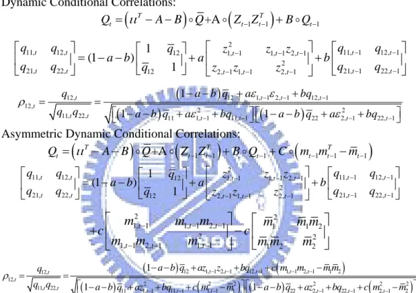
3.5 The Dynamic Conditional Correlation (DCC) Model ... 15

3.6 The Asymmetric Dynamic Conditional Correlation (ADCC) Model ... 20

Ⅳ. Results ... 21 4.1 Data ... 21 4.2 Descriptive Statistics ... 22 4.3 Empirical Analysis ... 24 Ⅴ. Conclusion ... 30 Appendix A: ... 32 Appendix B: ... 33 References ... 34

List of Tables

Table 1: Descriptive Statistics ... 37 Table 2: Estimation Results of Bivariate Return-based (GARCH) and Range-based (CARR) DCC and ADCC Model. ... 39 Table 3: Estimation Results of Bivariate Return-based DCC and ADCC Model

with Asymmetry in Conditional Variance (GJR-GARCH) ... 41 Table 4: Comparison of the Volatility Values of Timing in the Minimum Variance

Strategy (GARCH-DCC vs. CARR-DCC) ... 43 Table 5: Comparison of the Volatility Values of Timing in the Minimum Variance

Strategy (GARCH-ADCC vs. CARR-ADCC) ... 44 Table 6: Comparison of the Volatility Values of Timing in the Minimum Variance

Strategy (GJR-GARCH-DCC vs. GJR-GARCH-ADCC) ... 45 Table 7: Comparison of the Incremental Volatility Values of Timing in the

Minimum Variance Strategy. ... 46

List of Figures

Figure 1: S&P 500 Index and 10 Year Treasury Bond Weekly Closing Prices,

Returns, Ranges, Open Interests and Trading Volumes. ... 49 Figure 2: Volatility Estimates for the GARCH, GJR-GARCH and CARR Model . 51 Figure 3: Correlation and Covariance Estimates for the DCC and ADCC fitted by

GARCH, CARR and GJR-GARCH ... 54 Figure 4: The Weights of Minimum Volatility Portfolio Derived by the Static and

Ⅰ. Introduction

Modern portfolio theory (MPT) proposes how rational investors use diversification to allocate their assets and optimize their portfolios. MPT models a portfolio as a weighted combination of assets so that the return of a portfolio can be expressed as a summation of the constituent asset’s returns. Additionally, the volatility of a portfolio (σ2portfolio) can be

shown as the function of the variance of each asset (σi2) and the correlation (ρij) of the

component assets. One of the most influential concepts of MPT is Markowitz diversification. Diversification in investment portfolio is a risk management technique that mixes a wide variety of assets within a portfolio. Because the fluctuations1 of a single asset have less impact on a diversified portfolio, diversification can eliminate the specific-risks or unsystematic-risks from any one investment portfolio. In order to reduce the specific-risks of a portfolio, one can invest multiple assets with varied risk levels, therefore, large losses in some assets are offset by others assets if their correlations are not equal to one (perfectly correlated). In other words, investors can reduce their exposure to individual asset risk by holding a diversified portfolio of assets. Although diversification minimizes the risk of a portfolio, it does not necessarily reduce the portfolio return. Consequently, well-diversified in assets is referred to as the free lunch in finance.

In Markowitz portfolio selection model, we can generalize the portfolio construction problem to the case of many risky assets and a risk-free asset. The first step is to determine the return-risk trade-off to the investor. There are summarized by the minimum-variance frontier. This frontier is a graph of the lowest possible portfolio variance that is attainable for a given portfolio expected return. Afterward we can easily find the weights of global

1

More volatile of fluctuations, more risk of assets. We use the standard deviation of the portfolio’s return to proxy the portfolio risk in this study.

minimum variance portfolio with the function of each asset’s variance (σ_i2) and the

covariance (σ_ij) between two constituent assets. The part of the frontier that lies above the

global minimum-variance portfolio is called the efficient frontier of risky assets. The second part of the optimization includes the risk-free asset proxied by an investment in short-dated Government securities. The risk-free asset has zero variance in returns, and it is uncorrelated with any other asset. Accordingly, we search for the capital allocation line (CAL) with the highest reward-to-variability ratio (Sharpe ratio, S ), and the CAL must be _p tangent to the efficient frontier. Sharpe ratio is a measure of the excess return (risk premium) per unit of risk. Therefore, the portfolio is the optimal risky portfolio with more than two risky assets and a risk-free asset. For the weights that result in risky portfolio with the highest Sharp ratio, the objective is to maximize the slope of the CAL for any possible portfolio.

A number of useful improvements have appeared since the moment of the classic theory creation. In static portfolio strategy, we can employ the unconditional expected returns (u ), variances (_i σ_i), and correlations (ρ_ij) for any target return (u_target) to acquire the optimal weights of risky and risk-free assets in our portfolio. The MPT uses the historical parameter “volatility” as a proxy for risk and assumes volatility never changes. The optimal weights of the portfolio are not dynamic because we don’t take the time-varying character into account.

Recently, quantitative investment becomes popular in financial market. Investors and quantitative analysts begin using mathematical and statistical models to price stocks, bonds and derivatives. Dynamic investment strategies used in portfolio optimization would benefit investors because the financial markets are not entirely efficient and the phenomenon of volatility is changeable over time. In another word, dynamic investment strategies not only

reduce the risk but improve portfolio performance as well.

In the financial market, the financial economists found that the autocorrelation plays an important role in estimating volatility than in estimating return. Therefore, we can forecast the second moment such as volatility and correlation easily than the first moment (return). Previous researchers had assumed constant volatility and used simple devices to approximate risk. Engle (1982) proposed the Autoregressive Conditional Heteroscedasticity (ARCH) model in which the variance at time t (σ_{i t}2_, ) is modeled as a linear combination of

the past q-period of squared errors (ε_{t q}2₋ ). Afterward, Bollerslev (1986) added lag lengths p

of variance (σ_{i t p}2_,− ) to the model and advanced the GARCH (Generalized ARCH) model for measuring and forecasting financial market volatility. The GJR-GARCH model with asymmetry was introduced by Glosten, Jaganathan, and Runkle (1993) following the GARCH model. In the GJR-GARCH model, good news (ε_{t q−} > ) and bad news (0 ε_{t q−} < ) 0 have different effects on the conditional variance, the model suggests that bad news increases volatility more than good news in general.

The above-mentioned GARCH family models are based on the return data (log_e

(

p_tclose p_tclose₋₁

)

). Recently, numerous studies have mentioned that the range data based on the logarithmic difference of high and low prices in a fixed interval (log_e

(

p_thigh p_tlow

)

) make a superior estimation of volatility than the return data. Parkinson pioneered in estimating the variance of the rate of return (see Parkinson, 1980). The follow-up studies are Brandt and Jones (2006), Chou (2005, 2006) and Martens and Dijk (2007). Especially, Chou (2005) proposed a Conditional Autoregressive Range (CARR) model which provides sharper volatility estimates compared with the standard GARCH model.

of individual asset into account, but the conditional covariance and correlation as well. Engle developed new econometric models of volatility that captured the tendency of more than two assets to move between high volatility and low volatility period. Engle (2002a) advanced the Dynamic Conditional Correlation (DCC) Model, which is derived from the GARCH family.

In the recent, researchers have noted that volatilities and correlations for financial markets rise more after negative returns shocks than after positive shocks. Namely, the asymmetric phenomena of volatility and correlation show that there are higher market volatility and correlation levels in market downswings than in market upswings. Cappiello, Engle, and Sheppard (2006) proposed the ADCC (Asymmetric DCC) model to capture the asymmetry in estimating dynamic correlations.

The existence of asymmetry has been widely studied and confirmed. It plays a vital role in risk management and asset allocation. From the viewpoints of investors, the main issue is whether asymmetric phenomenon can reduce the volatility, enhance risk-adjusted portfolio return and improve utility of investors.

In the mean-variance framework, investors acquire the different portfolio weights over time using varied models. Therefore, we can easily obtain the return and risk of the optimal portfolio. In order to measure the economic value of timing under uncertainty, we consider an investor with different risk-averse levels uses conditional volatility and correlation to allocate portfolio among cash, stock, and bond. Fleming, Kirby and Ostdiek (2001) extended West, Edison, and Cho’s (1993) utility criterion to measure the economic value of timing with different risk tolerance levels. This study shows that the CARR model may bring out a better performance to investor, that is to say, the investor might pay more annually to switch from the static strategy to the dynamic strategy.

The article is structured as follows. In Section Ⅱ, we introduce literature related to GARCH family and CARR with DCC and ADCC model. In addition, the literature resources related to the economic value of timing are also included in Section Ⅱ. Section Ⅲ provides the methodology of asset allocation, the measurement of economic value over time, and the return-based (GARCH and GJR-GARCH) and range-based (CARR) models with DCC and ADCC. Section Ⅳ presents the data used in this paper, its summary statistics, and the details of the performance in the different strategies and risk aversion levels. Finally, Section Ⅴ is the conclusion to the paper.

Ⅱ. Literature Review

2.1 The Mean-Variance Framework

Prior to Markowitz's work, investors focused on assessing the risks and returns of individual securities in constructing their portfolios. Markowitz (1952) proposed that investor focus on selecting portfolio based on their overall risk-return characteristics.

Tobin (1958) expanded on Markowitz’s framework by adding a risk-free asset to the portfolio. This made it possible to leverage or deleverage portfolio on the efficient frontier. Through leverage, portfolio on the capital allocation line that outperform portfolio on the efficient frontier is feasible.

2.2 The Value of Volatility Timing Measurement

Many studies show that the forecast models only can explain little part of variations in time-varying volatilities. Some studies argue against the viewpoints and wonder whether volatility timing has economic value (Busse (1999), Fleming, Kirby, and Osdiek (2001, 2003), Marquering and Verbeek (2004)).

This article focuses on whether range-based models are superior to return-based models, and investors are willing to switch from a symmetric DCC to an asymmetric DCC model. The purpose of this paper is to examine its economic value of volatility timing by using conditional mean-variance framework developed by Fleming, Kirby and Ostdiek (2001).

We construct three-asset, mean-variance portfolio made up of two market returns (stock and bond) and the risk-free asset (cash). Fleming, Kirby and Ostdiek (2001) extend West, Edison, and Cho’s (1993) utility criterion to test the economic value of volatility

timing for the short-horizon investors with different risk tolerance levels. In this paper, we examine the economic value for longer horizon forecast of selected models in our empirical study.

2.3 The ARCH, GARCH and GJR-GARCH Model

The Autoregressive Conditional Heteroskedasticity (ARCH) model has become the most famous model in processing the conditional volatility since Engle (1982) proposed it. The ARCH model adopts the effect of past residuals and helps explain the volatility clustering phenomenon. In traditional econometrics models, the one period forecast variance is assumed to be constant. The ARCH model differently assumes that variance of residuals to be time varying and conditional on past sample. Bollerslev (1986) proposed the Generalized ARCH (GARCH) model which brings the previous volatility term into the ARCH model. The GARCH model opens a new field in research of volatility and is widely applied in research of financial and economic time series.

The GJR-GARCH model with asymmetry was introduced by Glosten, Jaganathan, and Runkle (1993) following the GARCH model. In the GJR-GARCH model, good news and bad news have different effects on the conditional variance, the model suggests that bad news increases volatility more than good news in general.

2.4 The Conditional Autoregressive Range (CARR) Model

Several studies show that the range data can offer a sharper estimate of volatility than the return data. A number of studies have investigated this issue started with Parkinson’s (1980) research, and more recently, Brandt and Jones (2006), Chou (2005, 2006), and Martens and Dijk (2007). Especially, Chou (2005) proposes a Conditional Autoregressive Range (CARR) model which can easily capture the dynamic volatility structure and has obtained some

insightful empirical evidences.

2.5 The Dynamic Conditional Correlation (DCC) and Asymmetric Dynamic Conditional Correlation (ADCC) Model

Bollerslev (1990) presents the Constant Conditional Correlation (CCC) model uses a strong assumption, the correlation of variables to be fixed, to simplify the estimation process. Kroner and Ng (1998) propose the General Dynamic Conditional Correlation model which incorporates several multivariate GARCH models to compose a more general model. Engle (2002a) looses the restriction of constant conditional correlation and proposes Dynamic Conditional Correlation (DCC) model.

In the ADCC (Cappiello, Engle and Sheppard 2006) model, both conditional variance and correlation increase in response to negative news, allowing portfolio weights computed from ADCC.

Ⅲ. Model

3.1 Mean-Variance Framework

Mean-variance optimization (MVO) is a quantitative tool which allows investors to optimize their portfolios by considering the risk/return trade-off. In conventional single period MVO, investors make optimal portfolio decision for a single forthcoming period. The objective is to minimize portfolio risk (variance) subject to a selected level of target return. The single period MVO was developed by Markowitz.

In the beginning, we consider a minimization problem for the portfolio variance ( 2

portfolio

σ ) which is a measure of portfolio risk subjected to a target return constraint (μ_target).

Suppose R_t+1= ⎣⎡R_1,t+1LR_{k t,+1}⎤_⎦T denotes the expected return for each risky asset2, and

[ ]

1 , 1 1 n t i i t i E R w R μ _{+ +} =

= =

∑

denotes the expected return for portfolio. In addition, its conditional covariance matrix H for each risky asset is defined as follows, _t

(

)(

)

2 2 11, 1 1 , 1 1 1 2 2 1, 1 kk, 1 t k t T t t t t k t t H E R R σ σ μ μ σ σ + + + + + + ⎡ ⎤ ⎢ ⎥ ⎡ ⎤ = _⎣ − − _{⎦= ⎢ ⎥} ⎢ ⎥ ⎣ ⎦ L M O M L (1)

The matrix given above is a square matrix3 where its elements on the main diagonal are the variances of each risky asset. The top-right and bottom-left off-diagonal elements are the covariances between any two risky assets.

A single-horizon investor chooses the optimal weights of portfolio (w_t) to minimize portfolio variance subject to a target return constraint (μ_target), the minimization problem

2

In linear algebra, matrix AT indicates the transpose of a matrix A. 3

means that the portfolio of risky assets has the lowest variance. It can be expressed as follows, min t w 2 2 11, 1 1 , 1 1, 2 , 1, , 2 2 1, 1 kk, 1 , t k t t T portfolio t t t t t k t k t t k t w w H w w w w σ σ σ σ σ + + + + ⎡ ⎤ ⎡ ⎤ ⎢ ⎥ ⎢ ⎥ ⎡ ⎤ = _{= ⎣ ⎦ ⎢ ⎥ ⎢ ⎥} ⎢ ⎥ ⎢_⎣ ⎥_⎦ ⎣ ⎦ L L M O M M L

(

)

target subject to w_tT

μ

+ −1 w_tT1 R_f =

μ

(2) where w_t = ⎣⎡w_1,tLw_{k t,} ⎤_⎦T is a k×1 vector of portfolio weights on the risky assets at time t,

f

R is the return on the risk-free asset, and μtarget is the given target return. The solution to the vector of optimal portfolio weights is as follows,

1 arg 1 ( ) ( 1) ( 1) ( 1) t et f t f t T f t f R H R w R H R μ μ μ μ − − − − = − − (3)

It is apparently to be expressed in a bivariate case (k=2): 4

(

2

)

target 1 2, 2 12, 1, 2 2 2 2 1 2, 2 1, 2 1 2 12, t t t t t t w μ μ σ μ σ μ σ μ σ μ μ σ − = + − ,

(

2

)

target 2 1, 1 12, 2, 2 2 2 2 1 2, 2 1, 2 1 2 12, t t t t t t w μ μ σ μ σ μ σ μ σ μ μ σ − = + − (4)

where μ_target =μ_target −R_f, μ₁=R₁−Rf, and μ2=R2−Rf are the excess target returns and

the excess returns of risky asset A and risky asset B.

3.2 Measuring the Value of Volatility Timing

West, Edison, and Cho (1993) make use of the quadratic utility function in exchange rate volatility measurement. According to their study, the investor’s utility can be defined as follows,

(

)

t+12 t+1 t+1 W U W =W 2 α － (5) 4 See Appendix A

where W is investor’s wealth at time t+1, _t+1 α is the Arrow-Pratt measure of absolute risk aversion (ARA) or coefficient of absolute risk aversion, the ARA is defined as follows,

(

)

₍

(

t+1

₎

)

t+1 t+1 t+1 U W ARA W U W 1 W α α ′′ = − = − ′ − (6)

The higher the curvature of U W

(

_t+1

)

, the higher the risk aversion. In addition, the Arrow-Pratt measure of relative risk aversion (RRA) is defined as follows,

(

)

t+1

₍

(

₎

t+1

)

t+1 t+1 1 t+1 t+1 W U W W RRA W U W 1 W t α γ α + ′′ = = − = − ′ − (7)

Under the measure of RRA, even if investor’s risk aversion changes from risk-averse to risk-loving, the measure is still a valid estimation. In order to capture the trade-off between risk and return, Fleming, Kirby and Ostdiek (2001) use a generalization of West, Edison, and Cho’s (1993) criterion to construct the linkage between quadratic utility and mean-variance framework. According to their study, the investor’s realized utility function at period t + 1 can be written as,

(

)

2 2 t+1 t , 1 , 1 W U W =W 2 t p t p t R ₊－α R ₊ (8)

where W is the investor’s wealth at period t and the portfolio return (_t R_{p t,+1}) at period t+1 is defined as follows,

(

)

1, 1 , 1 1 1 1, , , 1 1 1 t T T T p t t f t t f t t f t k t k t r R w R w R R w r R w w r + + + + + ⎡ ⎤ ⎢ ⎥ ⎡ ⎤ = − + = + = _{+ ⎣ ⎦ ⎢ ⎥} ⎢ ⎥ ⎣ ⎦ L M (9)

1

t

r₊ is defined in terms of excess returns, it can be expressed as follows,

1, 1 1, 1 1 1 , 1 , 1 1 t f t t t f k t f k t R R r r R R R R r + + + + + + ⎡ − ⎤ ⎡ ⎤ ⎢ ⎥ ⎢ ⎥ = − =_{⎢ ⎥ ⎢}= _⎥ ⎢ − ⎥ ⎢_⎣ ⎥_⎦ ⎣ ⎦ M M (10)

For comparison between the static and dynamic investment strategies, we assume that the investor has a constant relative risk aversion (CRRA), that is to say γ_t is equal to some

fixed value γ . This implies αW_t is also a constant term.

t t W W W= 1 W 1 W 1+ t α α γ γ γ α α α γ = ⇒ = ⇒ − − (11)

The equation (8) can be rewritten as

(

)

₍

t

₎

2

₍

₎

2 t+1 t , 1 , 1 t , 1 , 1 W U W =W W 2 1 2 1 p t p t p t p t R γ R R γ R γ γ + + + + ⎛ ⎞ = ⎜_⎜ ⎟_⎟ + _⎝ + _⎠ － － (12)

Under the assumption of CRRA, we can make use of the average realized utility U

( )

⋅

to estimate the expected utility by a given initial wealth W . ₀

( )

₍

₎

2 0 , , 1 W 2 1+ T p t p t t U R γ R γ = ⎛ ⎞ ⋅ = ⎜_⎜ − ⎟_⎟ ⎝ ⎠

∑

(13)

In order to estimate the value of volatility timing (Δ ), we equate the average utilities for any two alternative portfolios. The expression is as follows,

(

)

(

)

(

)

(

)

2 2 , , , , 1 2 1 1 2 1 T T a t a t b t b t t t R γ R R γ R γ γ = = ⎡ ⎤ ⎡ ⎤ − = − Δ − − Δ ⎢ ₊ ⎥ ⎢ ₊ ⎥ ⎣ ⎦ ⎣ ⎦

∑

∑

(14)

strategies, and Δ is the weekly maximum performance fee that an investor would be willing to pay to switch from one strategy to another.

In this paper, we use ordinary least square (OLS) model to represent the static investment strategy. On the contrary to the above-mentioned OLS strategy, we use three models, GARCH, GJR-GARCH and CARR model to measure the volatilities of individual assets. Additionally, in order to capture the time-varying relation among multiple assets, we employ the DCC and ADCC model to quantify their correlations and covariances.

To measure the weekly switching fee (Δ_weekly), we find the value of switching fee that

satisfies5 ( ) ( ) ( ) ( ) ( ) ( ) 2 2 2 , , , , , , 1 1 1 1 1 1 2 1 1 1 2 1 2 1 1 T T T T T T b t b t a t a t b t b t t t t t t t weekly R T R T T R R R R T γ γ γ γ γ γ γ γ γ γ γ γ = = = = = = ⎡ ⎤ ⎛ ⎞ ⎛ ⎞ ⎛ ⎞ ⎛ ⎞ ⎛ ⎞ − ± − − ⎢ − − − ⎥ ⎜ ₊ ⎟ ⎜ ₊ ⎟ ⎜ ₊ ⎟ ⎜ ₊ ⎟ ⎜ ₊ ⎟ ⎢ ⎥ ⎝ ⎠ ⎝ ⎠ ⎝ ⎠ ⎝⎣ ⎠ ⎝ ⎠⎦ Δ = + ∑ ∑ ∑ ∑ ∑ ∑ (15)

We report our estimates of switching fee annually (Δ_annually) using three different values of relative risk aversion (RRA), that is γ = , 1 γ = and 5 γ =10.

3.3 The ARCH, GARCH and GJR-GARCH Model

In the Gauss–Markov theorem, it assumes that all error terms have the same variance (Var

( )

ε_i =σ2), that is homoscedasticity. But in the financial market, it is observed that the variance has the phenomenon of volatility clustering which was documented by Mandelbrot. Volatility clustering is a pervasive feature in many securities markets, observations of this type in financial time series are usually approached by ARCH-type models.

5

Engle (1982) first proposes the Autoregressive Conditional Heteroskedasticity (ARCH) model. It the ARCH model, it allows the conditional variance (h_t) to vary over time as a function of past information (ε_{t i}2₋ ). After that, Bollerslev (1986) advances the Generalized ARCH (GARCH) model based on the ARCH model. The GARCH (p, q) is defined as follows,

(

)

1 , | ~ 0, t t t t t r = +μ ε ε Ω₋ N h (16) 2 1 1 q p t i t i i t j i j h ω α ε ₋ βh₋ = = = +

∑

+

∑

(17) where the equation (16) and (17) are the conditional mean equation and conditional variance equation, respectively. Ω is the information set at time t-1, t−1 N

(

0,ht

)

shows

the normal distribution with a mean of zero and a variance of h_t, ω is a constant term, and ε_{t i}2₋ (ARCH term) is the news about volatility from the lag lengths q period while

t j

h₋ (GARCH term) is the lag lengths p period’s forecast variance.

GJR-GARCH was introduced by Glosten, Jaganathan, and Runkle (1993). The generalized specification for the conditional variance of GJR-GARCH (p, q, r) is given by,

2 2 1 1 1 q p r t i t i i t j k t k t k i j k h ω α ε₋ βh₋ δ I₋ ε₋ = = = = +

∑

+

∑

+

∑

where 1, 0 0, 0 t t t I ε ε < ⎧ = ⎨ _≥ ⎩ (18)

In the GJR-GARCH model, good news has an impact of α_i while bad news has a great effect of α δi+ k t kI− on the conditional variance. In the GARCH equation, δk is restricted to

zero, i.e. the GARCH model is the special case of the GJR-GARCH model. In the GJR-GARCH model, bad news will increase volatility and has asymmetric impact when

0

k

3.4 The Conditional Autoregressive Range (CARR) Model

Chou (2005) proposed the Conditional Autoregressive Range (CARR) model to estimate the volatility of financial assets. The range (R ) is a better estimator of standard deviation (i t, σt)

in statistics and is defined as R_{i t,} =log_e

(

P_{t i,}high p_{t i}low_,

)

. The CARR (p, q) for the range can be expressed as follows, 1 , | ~ exp(1, ) t t t t t R =λ ε ε Ω₋ ⋅ , 1 1 q p t i t i j j t j i j R λ ω α ₋ β λ ₋ = = = +

∑

+

∑

(19) * / c t t t z =r λ ，where * t adj t λ = × ，λ ˆ adj σ λ =

where the range R is calculated by the difference between logarithm high and low prices _t during a fixed interval. λ_t and λ are the conditional and unconditional mean of the range, ˆ respectively. ε_t is the disturbance term, or the normalized range (ε_t =R_t λ_t ), which is assumed to follow the exponential distribution. σ is the unconditional standard deviation for the return series. The ratio of adj is used to adjust the range (λ_t) to produce the standardized residuals (z_tc =r_t/

(

adj×λ_t

)

).

3.5 The Dynamic Conditional Correlation (DCC) Model

The Dynamic Conditional Correlation (DCC) model (Engle 2002a) can be viewed as an extension of the Bollerslev (1990) constant conditional correlation (CCC) model. In Bollerslev’s CCC model, the covariance matrix H for a vector of k asset returns can be _t written as follows,

2 11, 1 , 2 1, , t k t t t t k t kk t h h H D RD h h ⎡ ⎤ ⎢ ⎥ = _{= ⎢ ⎥} ⎢ ⎥ ⎣ ⎦ L M O M L (20)

where R is the sample correlation matrix and D_t is the k k× diagonal matrix, a diagonal matrix is a square matrix where the entries outside the main diagonal are all zero. The diagonal matrix D_t can be defined as,

{ }

11, , , 0 0 t t ii t kk t h D diag h h ⎡ ⎤ ⎢ ⎥ = _{= ⎢ ⎥} ⎢ ⎥ ⎣ ⎦ L M O M L (21) , ii t h for the th

i return series on the th

i diagonal are time-varying standard deviations generated from univariate GARCH model. h_{ii t,} is the square root of the estimated variance. The following expressions report the covariance matrix H of CCC model in t

great detail. 11, 11 1 11, 11, 1 11, , 1 , , 1 , 0 0 0 1 0 0 0 0 1 0 t k t t k t t t t kk t k kk kk t kk t k kk t h h h h H D RD h h h h ρ ρ ρ ρ ρ ρ ⎡ ⎤⎡ ⎤⎡ ⎤ ⎡ ⎤⎡ ⎤⎡ ⎤ ⎢ ⎥⎢ ⎥⎢ ⎥ ⎢ ⎥⎢ ⎥⎢ ⎥ = =_{⎢ ⎥⎢ ⎥⎢ ⎥ ⎢}= _{⎥⎢ ⎥⎢ ⎥} ⎢ ⎥⎢_⎣ ⎥_⎦⎢ ⎥ ⎢ ⎥⎢_⎣ ⎥_⎦⎢ ⎥ ⎣ ⎦ ⎣ ⎦ ⎣ ⎦ ⎣ ⎦ L L L L L L M O M M O M M O M M O M M O M M O M L L L L L L 2 2 11, 11, , 1 11, 1 , 2 2 11, , 1 , 1 , , t t kk t k t k t t t t t kk t k kk t k t kk t h h h h h H D RD h h h h h ρ ρ ⎡ ⎤ ⎡ ⎤ ⎢ ⎥ ⎢ ⎥ = =_{⎢ ⎥ ⎢}= _⎥ ⎢ ⎥ ⎢ ⎥ ⎣ ⎦ ⎣ ⎦ L L M O M M O M L L (22)

The CCC model estimates the conditional covariance (H ) using the constant _t conditional correlation matrix ( R ) and the product of the two conditional standard deviations (D ). The drawback of the CCC model is that it’s assumption of constant _t conditional correlation is too restrictive and ignores the time-varying correlations.

Engle (2002a) proposes the DCC model to estimate the covariance matrix of multiple asset returns. The main distinction between the DCC model and the CCC model is whether the conditional correlation matrix changes over time or not. The DCC model allows R to t

11, 11, 1 , 11, 11, 1 , 11, , 1, , , , 1, , 0 0 0 1 0 0 0 0 1 0 t t k t t t k t t t t t t kk t k t kk t kk t kk t k t kk t h h h h H D R D h h h h ρ ρ ρ ρ ρ ρ ⎡ ⎤ ⎡ ⎤ ⎡ ⎤ ⎡ ⎤ ⎡ ⎤ ⎡ ⎤ ⎢ ⎥ ⎢ ⎥ ⎢ ⎥ ⎢ ⎥ ⎢ ⎥ ⎢ ⎥ = =_{⎢ ⎥ ⎢ ⎥ ⎢ ⎥ ⎢}= _{⎥ ⎢ ⎥ ⎢ ⎥} ⎢ ⎥ ⎢ ⎥ ⎢ ⎥ ⎢ ⎥ ⎢ ⎥ ⎢ ⎥ ⎣ ⎦ ⎣ ⎦ ⎣ ⎦ ⎣ ⎦ ⎣ ⎦ ⎣ ⎦ L L L L L L M O M M O M M O M M O M M O M M O M L L L L L L 2 2 11, 11, , 1 , 11, 1 , 2 2 11, , 1 , , 1 , , t t kk t k t t k t t t t t t kk t k t kk t k t kk t h h h h h H D R D h h h h h ρ ρ ⎡ ⎤ ⎡ ⎤ ⎢ ⎥ ⎢ ⎥ = =_{⎢ ⎥ ⎢}= _⎥ ⎢ ⎥ ⎢ ⎥ ⎣ ⎦ ⎣ ⎦ L L M O M M O M L L (23) { } { } { } 11, _{11, 1 ,} 11, 1 1 2 2 1, , , , 1 0 1 0 0 1 0 1 t _{t k t} t t t t t k t kk t kk t kk t q q q q R diag Q Q diag Q q q q q − − ⎡ ⎤_{⎡ ⎤}⎡ ⎤ ⎢ ⎥_{⎢ ⎥}⎢ ⎥ = = ⎢ ⎥_{⎢ ⎥}⎢ ⎥ ⎢ ⎥_{⎢ ⎥}⎢ ⎥ ⎣ ⎦ ⎢ ⎥ ⎢ ⎥ ⎣ ⎦ ⎣ ⎦ L _L L M O M M O M M O M L L L 1 , 11, , _{1 ,} 1, 1, 11, , 1 ₁ 1 1 k t t kk t _{k t} t k t k t t kk t q q q R q q q ρ ρ ⎡ _{⎤ ⎡ ⎤} ⎢ _{⎥ ⎢ ⎥} =⎢ _{⎥ ⎢}= _⎥ ⎢ _{⎥ ⎢ ⎥} ⎣ ⎦ ⎢ ⎥ ⎣ ⎦ L _L M O M M O M L L (24)

The conditional standardized residual vector Z and the conditional standardized residual _t covariance matrix Q_t = ⎣ ⎦ are expressed as follows, respectively, ⎡q_{ij t,} ⎤

1, , T t t k t Z = ⎣⎡z _L z ⎤_⎦ 1,t 1,t/ 1,t z =r h (25) where z is a standardized residual that has mean zero and variance one for each asset _{i t,} return series.

(

)

+A

(

1 1

)

1

T T

t t t t

Q = ιι − −A B _oQ _o Z Z_{− −} +B Q_{o −} (26) where ι is a vector of ones and o is the Hadamard product of two identically sized matrices, which is computed simply by element-by-element multiplication. To put it another way, the Hadamard product of two m n× matrices A and B is an m n× matrix given by

(

A Bo

)

ij =a bij ij . In addition, Q= ⎣ ⎦ means the unconditional covariance matrix of ⎡ ⎤qij

standardized residuals.

Q , Z Z_{t−1 t}T₋₁ and Q_t−1 in equation (26) are all nonnegative despite their time-varying attributes. In linear algebra, a real symmetric n n× matrix is said to be positive semi-definite (positive definite) if and only if all its eigenvalues are nonnegative (positive).

In our study, if ιιT − − , A and B matrices are all positive semi-definite, then A B Q_t will also be positive semi-definite. However, if any one of the matrices of ιιT − − , A A B and B is positive definite, then Q_t will also be positive definite.

The bivariate case for the time-varying covariance matrix and correlation matrix can be expressed as,

(

)

11, 12, 11 12 1, 1 11, 1 12, 1 1, 1 2, 1 21, 22, 21 22 2, 1 21, 1 22, 1 1 t t t t t t t t t t t t q q q q z q q a b a z z b q q q q z q q − − − − − − − − ⎡ ⎤ ⎡ ⎤ ⎡ ⎤ ⎡ ⎤ ⎡ ⎤ = − − + + ⎢ ⎥ ⎢ ⎥ ⎢ ⎥⎣ ⎦ ⎢ ⎥ ⎣ ⎦ ⎣ ⎦ ⎣ ⎦ ⎣ ⎦

(

)

(

)

(

)

(

)

2 11, 12, 11 1, 1 11, 1 12 1, 1 2, 1 12, 1 2 21, 22, 21 1, 1 2, 1 21, 1 22 2, 1 22, 1 1 1 1 1 t t t t t t t t t t t t t t q q a b q az bq a b q az z bq q q a b q az z bq a b q az bq − − − − − − − − − − ⎡ − − + + − − + + ⎤ ⎡ ⎤ = ⎢ ⎥ ⎢ ⎥ _{− − + + − − + +} ⎣ ⎦ ⎣ ⎦ (27)

(

)

(

)

(

)

12, 12 1, 1 2, 1 12, 1 12, 2 2 11, 22, _{11 1, 1 11, 1 22 2, 1 22, 1} 1 1 1 t t t t t t t _{t t t t} q a b q az z bq q q _{a b q az bq a b q az bq} ρ − − − − − − − − − + + = = ⎡ − − + + ⎤ ⎡ − − + + ⎤ ⎣ ⎦ ⎣ ⎦ (28) where

[ ]

[ ]

( ) ( )

1 2 12 1 2 12 2 2 1 2 E z z q E z z E z E z ρ = = =

The DCC model was designed to estimate by two-stage Quasi-Maximum Likelihood Estimation (QMLE) to obtain consistent parameter estimates. The log-likelihood can be expressed as the sum of the volatility component and the correlation component.

volatility correlation

L=L +L (29) The log-likelihood function of this estimator can be described as,

( )

(

1

)

1 1 log 2 log 2 T T t t t t t L k π H r H r− = = −

∑

+ +

( )

(

1 1 1

)

1 1 log 2 log 2 T T t t t t t t t t t k π D R D r D R D r− − − = = −

∑

+ +

( )

(

1

)

1 1

log 2 2 log log 2 T T t t t t t t k π D R Z R Z− = = −

∑

+ + + since Z_t =D r_t−1_t (30)

( )

(

1 1 1 1 1

)

1 1

log 2 2 log log

2 T T T T t t t t t t t t t t t t t t k π D r D D r− − r D D r− − R Z R Z− = = −

∑

+ + − + +

( )

(

1 1 1

)

1 1

log 2 2 log log

2 T T T T t t t t t t t t t t t t k π D r D D r− − Z Z R Z R Z− = = −

∑

+ + − + +

Let the parameters in Dt be denoted θ and the parameters in Rt be denoted φ.

The log-likelihood function can be divided into two-stage estimation.

( )

, _volatility

( )

_correlation

( )

,

L θ φ =L θ +L θ φ (31) In the first stage, we estimate the volatility term which univariate GARCH models are estimated for each residual series. In the second stage, we use residuals which transformed by their standard deviation estimated during the first stage to estimate the parameters of the dynamic correlation. The former term in equation (31) denotes the volatility part, and the latter term is the correlation part.

( )

(

( )

1 1

)

1 1 log 2 2 log 2 T T volatility t t t t t t L θ k π D r D D r− − = = −

∑

+ + (32)

( )

(

1

)

1 1 , log 2 T T T correlation t t t t t t t L θ φ R Z R Z− Z Z = = −

∑

+ + − (33) When the specific GARCH model is fitted, the volatility part of the likelihood function is apparently the sum of individual GARCH likelihood functions. It can be demonstrated as,

( )

( )

2, , 1 1 , 1 log 2 log 2 T k i t volatility i t t i i t r L h h π = = ⎛ ⎞ = − ⎜_⎜ + + ⎟_⎟ ⎝ ⎠

∑∑

(34)

To maximize the likelihood function in the first stage, we can find the optimal parameter of θ . ˆ

( )

{

}

ˆ _{arg max} volatility L θ = θ (35)

and then take this value of θˆ as given in the second stage to estimate the maximum value of likelihood function and its optimal parameter φ.

( )

{

ˆ

}

max L_correlation ,

3.6 The Asymmetric Dynamic Conditional Correlation (ADCC) Model

In this paper, we model the conditional correlation matrix Rt with asymmetry following

Cappiello, Engle, and Sheppard (2006). By using the standardized residuals (z ), we are able _t to estimate asymmetric dynamic conditional correlation matrices of the form,

{ } { }

1

{ }

1

2 2

t t t t

R =diag Q − Q diag Q − (37) and the asymmetric term (ADCC) setup is,

(

)

+A

(

1 1

)

1

(

1 1 1

)

T T T

t t t t t t t

Q = ιι − −A B _oQ _o Z Z_{− −} +B Q_{o −} +C_o m m_{− −} −m₋ (38) where A, B, and C are scalar parameters. Q_t= ⎣ ⎦⎡q_{ij t,} ⎤ and Q= ⎣ ⎦⎡ ⎤q_ij are the conditional and

unconditional covariance matrix of standard residual vector ( Z_t ). The vector

[

0

]

t t t

m = Ι Z < oZ and m=1T

∑

m m_t T_t . Hence, conditional correlation ρ_12,t can easily be solved immediately. In a bivariate case, the covariance matrix and correlation in the ADCC model can be expressed as follows,

2 11, 12, 12 1, 1 1, 1 2, 1 11, 1 12, 1 2 21, 22, 12 2, 1 1, 1 2, 1 21, 1 22, 1 1 (1 ) 1 t t t t t t t t t t t t t t q q q z z z q q a b a b q q q z z z q q − − − − − − − − − − ⎡ ⎤ ⎡ ⎤_{= − −} ⎡ ⎤_{+ +} ⎡ ⎤ ⎢ ⎥ ⎢ ⎥ ⎢ ⎥ ⎢ ⎥ ⎣ ⎦ ⎣ ⎦ ⎣ ⎦ ⎣ ⎦ 2 2 1, 1 1, 1 2, 1 1 1 2 2 2 1, 1 2, 1 1, 1 1 2 2 t t t t t t m m m m m m c c m m m m m m − − − − − − ⎡ ⎤ ⎡ ⎤ + _{⎢ ⎥}− _{⎢ ⎥} ⎣ ⎦ ⎣ ⎦ (39)

(

)

(

)

(

)

(

)

(

)

(

)

12 1, 1 2, 1 12, 1 1, 1 2, 1 1 2 12, 2 2 2 2 2 2 11 1, 1 11, 1 1, 1 1 22 2, 1 22, 1 2, 1 2 1 1 1 t t t t t t t t t t t t a b q az z bq c m m m m a b q az bq c m m a b q az bq c m m ρ − − − − − − − − − − − − − + + + − = ⎡ _{− − + + + −} ⎤ ⎡ _{− − + + + −} ⎤ ⎣ ⎦ ⎣ ⎦

Ⅳ. Results

4.1 Data

In this section, we examine U.S. stock and bond weekly returns and weekly ranges spanning the period from January 1, 1990 to April 25, 2008. The data employed for our empirical study consist of 956 weekly observations on the Standard & Poor’s 500 Composite Index Futures (henceforth S&P 500 futures), and 10-year U.S. Treasury bond Futures (henceforth 10-year T-bond futures). S&P 500 futures contract was developed by Chicago Mercantile Exchange (CME), CME is a financial and commodity derivative exchange based in Chicago. The S&P 500 index is a stock market index comprising the 500 large-cap companies actively traded in the U.S. stock markets. It is the reason why we choose S&P 500 to represent the U.S. stock market. 10-year T-bond futures contract was introduced by Chicago Board of Trade (CBOT), T-bond futures contract meets our needs as we seek to manage the long-term risk. In this article, we employ futures prices data rather than spot prices data because of the short sale constraints of spot market. In order to borrow stock shares in spot market, the investors need to find a stock owner willing to lend them. What is more, once an investor has a short-sale position by borrowing stock, the recall risk would happen to him at any time. Consequently futures contract enables us to avoid short sale constraints.

We retrieve the raw data of S&P 500 futures and 10-year T-bond futures for the entire period from Thomson Datastream financial statistical database. Thomson Datastream provides the futures prices on nearest contract and roll over to the second nearest contract when the nearest contract approaches maturity. The Treasury bill (henceforth T-bill) interest rates provided are supposed to be risk-free. Therefore we use the 3-month T-bill rate to substitute for the risk-free rate. The T-bill rate is available in the Federal Reserve Board.

In order to measure the economic value of volatility timing, we apply the futures data of S&P500 and 10-year T-bond futures as well as the risk-free rate data of T-bill to obtain the time-varying portfolio weights, returns and variances using different econometric models.

4.2 Descriptive Statistics

< Figure 1 is inserted about here >

Figure 1 shows the graphs for close prices (Panel A), returns (Panel B) and ranges (Panel C) of S&P 500 futures and 10-year T-bond futures over the sample period from January 1, 1990 to April 25, 2008. The data of weekly return on S&P500 futures and 10-year T-bond futures are computed by the difference of logarithm close prices on two continuous weeks, i.e. , 100 log

(

, , 1

)

close close

i t e i t i t

r = × P P ₋ . However, the data of weekly range on S&P 500 futures and 10-year T-bond futures are defined by the difference of the high and low prices in the same week, i.e., R_{i t,} =100 log× _e

(

P_{i t,}high P_{i t,}low

)

. It is often reported as a percentage (%) by multiplying the above calculation by 100. In each panel of Figure 1, the vertical axis represents the weekly close price, weekly return and weekly range respectively, while the horizontal axis represents the sample period from 1990 to 2008. Panel B (weekly returns) and Panel C (weekly ranges) show the phenomenon of volatility clustering, that is to say, large changes of stock price tend to be followed by large changes, of either sign, and small changes of stock price tend to be followed by small changes. Panel D reports the weekly open interests and trading volumes of S&P 500 futures and 10-year T-bond futures.

In the futures market, there is no assurance that a liquid market exists for offsetting a futures contract all the time. It is obvious that market liquidity exists in the futures market of S&P 500 and 10-year T-bond because trading volumes remain stable consistently and

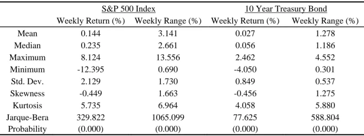
open interests increase gradually from 1990 to 2008. The descriptive statistics for the weekly return and range data of S&P 500 and T-bond are given in Table 1.

< Table 1 is inserted about here >

Table 1 shows the univariate statistics for the time series data over the sample period 1990-2008. The annualized value of mean and standard deviation are computed by

Mean 52× and Std. Dev× 52, therefore, the annualized values of mean (μ) and standard deviation (σ ) of S&P 500 futures (10-year T-bond futures) are 7.466% (1.414%) and 15.350% (6.120%). It is indicated that the weekly return data of S&P 500 futures is more volatile than 10-year T-bond futures by the individual standard deviations. But if we take coefficient of variation (CV =σ μ) into consideration, the CV of 10-year T-bond futures is 4.328 (CV_Tbond =σ_Tbond μ_Tbond =6.120% /1.414%) greater than the CV of S&P 500 futures (CV_SP500=σ_SP500 μ_SP500=15.350% / 7.466%=2.056). CV is a useful statistic for comparing the degree of variation among any time series data, even if the expected return are different from each other. Accordingly, the weekly return data of 10-year T-bond futures becomes more volatile if we take CV into account. That is to say, the lower ratio of standard deviation over expected return, the better our risk-return tradeoff. The expected weekly range (1.278%) of the 10-year T-bond futures prices is smaller than that (3.141%) of the S&P 500 futures prices. It is reasonable because the range is a proxy for measuring volatility.

For higher moments of the return and range data, the weekly return data of S&P 500 futures and 10-year T-bond futures are negative skewness (S =κ κ_{3 2}3 2=μ σ₃ 3<0). In another word, the distribution of return is concentrated on the right of the figure and the left tail is longer. In addition, all the data of weekly return and range are positive excess kurtosis,

the excess kurtosis statistic is defined as K =κ κ_{4 2}2− =3 μ σ₄ 4− . The distribution of 3 positive excess kurtosis has fatter tail characteristic with a higher probability of big positive and negative returns than the normal distribution. The Jarque-Bera (JB) statistic is used to test the null of whether the return and range data are normally distributed, based on the sample skewness and kurtosis. It is obvious that both data of weekly return and range reject the null hypothesis. In short, the sample moments for the return and range series of S&P 500 futures and the 10-year T-bond futures indicate sample distribution with fat tail and sharp peaks at the center compared to the normal distribution.

In the Panel B and Panel C of Table 1, it represents the unconditional covariance and correlation matrices between the time series date of S&P 500 futures and 10-year T-bond futures over the period from 1990 to 2008. The unconditional covariance matrices of return and range data are shown in Panel B. In the Panel C, it reports the unconditional correlation matrices between the S&P 500 futures and 10-year T-bond futures. The unconditional correlation coefficients of weekly return and range data between S&P 500 futures and 10-year T-bond futures are 0.016 and 0.114, respectively. Although the unconditional correlations are small, it does not imply their relations are very week. In our latter analysis, we will show the dynamic relationship of S&P 500 futures and 10-year T-bond futures.

4.3 Empirical Analysis

In order to deriving the optimal portfolio of two risky and risk-free assets, we employ the time-varying volatility models to estimate the conditional covariance and correlation. A static model does not specify the volatility over time, while a dynamic model does. Dynamic models are typically represented with difference equations. In this paper, we use ordinary least square (OLS) model to stand for the static model, and the dynamic models are represented by GARCH-DCC, GJR-GARCH-DCC, CARR-DCC, GARCH-ADCC,

GJR-GARCH-ADCC, and CARR-ADCC. The performance of dynamic model in comparison with that of static model is the main purpose in our study.

< Table 2 is inserted about here >

In the Table 2, it is documented the empirical results of the estimation with the GARCH-DCC, CARR-DCC, GARCH-ADCC, and CARR-ADCC model over the sample period from 1990 to 2008. We divide the table into two parts corresponding to the two steps in the DCC and ADCC estimation. We use GARCH and CARR model in the first step so that we can obtain the parameters fitted for DCC and ADCC model. In the first stage of Table 1 (Panel A), we can utilize the GARCH and CARR model fitted by return and range data with individual assets for attaining standardized residuals. Then, these standardized residual series can be brought into the second stage for dynamic conditional correlation (DCC) and asymmetric dynamic conditional correlation (ADCC) estimation. Panel B of Table 2 shows the estimated parameters of DCC and ADCC under the quasi-maximum likelihood estimation (QMLE).

< Table 3 is inserted about here >

Table 3 reports the estimation results of GJR-GARCH-DCC and GJR-GARCH-ADCC model using the weekly data of S&P 500 futures and 10-year T-bond futures. The estimation of GJR-GARCH-DCC and GJR-GARCH-ADCC model is similar to GARCH-DCC and GARCH-ADCC. The difference between GJR-GARCH and GARCH model is the measure of variance equation. The GJR-GARCH model proposed by Glosten, Jagannathan and Runkle (1993) incorporates the asymmetric effect of good news and bad news in the GARCH process on duration.

< Figure 2 is inserted about here >

Figure 2 provides the dynamic volatility of the S&P 500 futures and the 10-year T-bond futures based on the GARCH, GJR-GARCH and CARR model. Panel A (GARCH fitted), Panel B (GJR-CARCH fitted), and Panel C (CARR fitted) show the volatility estimates for the S&P 500 futures are abnormally high (solid line) in several periods. The East Asian Financial Crisis was beginning in 1997 followed by Russian financial crisis in 1998. Although it initially happened in Asian, the impact of financial crisis also had put pressure on the S&P 500 futures market in the United States. Moreover, the Dot-Com Bubble Crisis (Internet Bubble Crisis) took place in 2000 which led to the collapse in the technology industry as well as the overall financial market. After the collapse of the Dot-Com Bubble, there are terrorist attacks in September 11, 2001. The attacks had a great impact on the economy of U.S. and financial markets, the major stock exchanges like New York Stock Exchange (NYSE), American Stock Exchange (AMEX), and NASDAQ did not open on September 11 and remained closed until September 17. Besides, the stock market downturn was the dramatic decline in stock prices during 2002. The downturn can be regarded as sharp correction in the stock price after a decade-long bull market. In the meantime, a wave of accounting scandals became known to the public in the U.S., including Enron, Arthur Andersen, and WorldCom. In the third quarter of 2007, the U.S. subprime mortgage financial crisis had a great amount of impact on financial market of U.S. as well as other countries. The influence of subprime crisis is still ongoing, it seems like investors in the stock market are unsure of where to go with the money.

< Figure 3 is inserted about here >

Figure 3 reports the correlation and covariance estimates between S&P 500 futures and 10-year T-bond futures for the return-based (GARCH) and range-based (CARR) DCC and

ADCC model as well as the DCC and ADCC with GJR-GARCH model.

In Panel A, it appears that the dynamic conditional correlations become negative (ρ_12,t < ) at the end of 1997 no matter what the dynamic model we apply. In Panel B, the 0 time-varying correlations characteristic of GARCH-ADCC and CARR-ADCC are similar to the above-mentioned case in Panel A. Correlation is expressed by numbers ranging from -1 to +1. To eliminate diversifiable portfolio risk completely, we needs an intra-portfolio correlation approaches perfect inverse correlation (ρ_12,t = − ). Therefore, diversification 1 minimizes the risk of our portfolio well because S&P 500 futures prices have very low dynamic correlations with 10-year T-bond futures prices after the end of 1997, but it does not necessarily lower our expected return of portfolio.

Here we assume that investors use short-horizon mean-variance strategies to create portfolios from stock market (S&P 500 futures), bond market (10-year T-bond futures) and risk-free asset (T-bill rates). We construct the static portfolio (built by ordinary least square, OLS) using the unconditional mean (μ_i), variance (σ_i2) and covariance (σ_ij). Under the minimum variance framework, the weights of the portfolio are computed by the given target return, expected return, and conditional covariance matrices estimated by the GARCH-DCC and GARCH-ADCC, the GJR-GARCH-DCC and GJR-GARCH-ADCC, and the CARR-DCC and CARR-ADCC. Consequently, we can compare the economic value of the volatility models on 12 different target annualized return (5%~16%, 1% in an interval).

< Table 4 is inserted about here >

Table 4 reports how the economic values vary with the different target returns and the different constant relative risk aversions (CRRA). Panel A shows the annualized expected returns (μ), volatilities (σ) and Sharpe ratios (Sp) of the portfolios estimated from the

OLS, GARCH-DCC, and CARR-DCC model. For a quick look, the annualized Sharpe ratio (reward-to-variability ratio) calculated from the CARR-DCC (0.640) and GARCH-DCC (0.588) are higher than the OLS model (0.498). The advantages of using dynamic conditional correlation model to construct the portfolio are their better performance and smaller risk. Panel B shows the average annualized performance fees (△r) among the three models that a risk-averse investor would be willing to pay to switch from the static to the dynamic forecasting models. The values of CRRA are set to 1, 5, and 10, respectively. Roughly speaking, the switching fees raise consistently with higher target returns and higher constant relative risk aversions. Besides, Panel B also reports the performance fees if an investor change from the GARCH-DCC to the CARR-DCC model. Positive values for all cases show that CARR-DCC model dominates the GARCH-DCC model in forecasting conditional variances and correlations.

< Table 5 is inserted about here >

< Table 6 is inserted about here >

Table 5 gives a representation of the portfolio performance and switching fees that an investor would be willing to pay to switch from the symmetric GARCH-DCC and CARR-DCC to the asymmetric GARCH-DCC and CARR-DCC forecasting model. The results of GJR-GARCH-DCC and GJR-GARCH-ADCC model are displayed in Table 6.

< Table 7 is inserted about here >

Table 7 shows the incremental values of time-varying volatility among the OLS, GJR-GARCH-DCC, GJR-GARCH-ADCC, GARCH-DCC, CARR-DCC, GARCH-ADCC, and CARR-ADCC model using 5%, 10% and 16% target return respectively. In this paper,

we propose the asymmetric effect on the DCC model for the better performance. Panel A shows the volatility value with 5% target return. In the Panel A, the CARR-ADCC model has no superior as a dynamic forecasting model though there is no significant difference between CARR-DCC and CARR-ADCC model. Panel B and Panel C with the target return of 10% and 16% respectively show the opposite results of incremental value of volatility timing on model selection. In the Panel B as well as Panel C, the CARR-fitted models are better than the GARCH-fitted models, and the CARR-DCC is superior to the CARR-ADCC model.

<Figure 4 is inserted about here>

Figure 4 plots the weights of minimum volatility portfolio derived from static and dynamic models while setting the target return equal to 10%. The charts from Panel A to Panel F show the dynamic portfolio weights that minimize conditional volatility. In addition, Panel G has the constant portfolio weights for cash (-0.854), stock (1.360), and bond (0.494).

Ⅴ. Conclusion

In this paper, we extend the DCC model of Engle (2002a) with news impact in the conditional volatility and asymmetries in the dynamic correlation. We use three volatility models, GARCH, GJR-GARCH, and CARR model to go with the dynamic correlation models, DCC (symmetry) and ADCC (asymmetry). Therefore, we apply S&P 500 futures and 10-year T-bond futures to investigate whether asymmetries exist in conditional variances and correlations in the stock market and bond market of the U.S. The conditional volatilities of equity returns exhibit the asymmetric effects in the GJR-GARCH model while the little is found for bond returns. The performance of GJR-GARCH model is just better than OLS model, worse than the other dynamic models. We refer unfavorable performance in the GJR-GARCH model to its asymmetric effect in the stock return. Because of bad news has a great effect on the conditional variance that will increase the portfolio weights of 10-year T-bond. Furthermore, we examine the dynamic correlations of the S&P 500 futures and T-bond futures with DCC and ADCC model. Under consideration of asymmetric effect on conditional correlation, we find that the CARR-DCC and CARR-ADCC models are superior in the different target returns and risk aversions.

From the viewpoints of the investors, the above-mentioned models which mix rigorous mathematics and miraculous statistics are hard to understand for investors. The investors prefer the simplicity of investment strategy to the complexity of quantitative model. For that reason, the investors may choose the best quantitative model to allocate their assets and optimize their portfolio. In this paper, the investors may choose the CARR models as their quantitative methods in investment management since the CARR models lead to the better economic value of volatility. What is more, the economic value of volatility (switching fee) in this article is similar to “Two and Twenty” in hedge fund, this phrase indicates hedge

fund mangers charge a 2% of total asset value as a management fee, and an additional 20% of profits earned.