以適應性方法探討緊急救援服務的動態車輛派遣問題
摘要 在任何緊急情況下,人命的救援優於一切。當有事件發生時,急救服務必須在最短時 間到達現場。分派與調派模型目的在於把空閒的救護車分佈好以加强以後之派遣,而 哪一輛車應被派遣到現有的需求點則要一個有效的派遣策略。現有一般的救護車派遣 均採用“先到先服務”為原則,但這有可能做成次要受傷的人比有生命危險的先送達醫 院處理的情況發生。事實上救援分流已於一些地方實行,成效也不俗。本研究提出以“ 在有限資源及救援分流下,派遣最接近之救護車往最近之需求點不一定是最好”為出發 點,發展出一套更有效率之派遣模型,並延伸已有的派遣要素在救護車派遣問題上。 關鍵字︰ 救護車分派與調派; 動態車輛派遣; 動態規劃; 急救服務; 歷史訊息; 病 人分流An adaptive approach to the dynamic vehicle dispatching problem
with an application to emergency medical services
Abstract
When there is an incident, emergency service must be provided at the scene as quickly as possible with minimum delay. In many cities, there is a statutory obligation for the ambulance service to arrive within a certain limit of time. A current practice of such dispatching is on a First-Come-First-Served basis. As a result, patients with critical illness who call later may have to wait whilst less serious cases are taken to hospital first. In this research, we show that sending the nearest ambulance to the newly arrived request is not efficient under limited resources, given that patients are prioritized. The problem is formulated as a real-time dispatching model which is solvable by an adaptive dynamic programming approach. The results demonstrate that the overall system efficiency can be improved with increasing the system capacity and reducing the delay.
Keyword: Ambulance location and relocation; Dynamic vehicle dispatching; Dynamic programming; Emergency service; Historical information; Triage of patients
INTRODUCTION AND BACKGROUND
In emergency situations, a high priority must be placed on saving life. When there is an incident, emergency services, comprising police, fire fighters and ambulance services, must be provided at the scene as quickly as possible. This paper concerns ambulance dispatching. In many cities, there is a statutory obligation for the ambulance service to arrive on scene within a certain time limit. For example, the United States Emergency Medical Services Act requires that in urban areas 95% of requests should be reached within 10 minutes, while those in rural areas should be served within 30 minutes (see Ball and Lin, 1993). In United Kingdom, the target set by the London Ambulance Services for immediate life-threatening calls is 8 minutes (Thakore et al., 2002). In Japan, average time of ambulance arrival on site is about 6 minutes. To help meet these targets, ambulance location, allocation and relocation models are necessary. In general, location models determine the server or facility locations where the ambulances are dispatched from; allocation models decide which vehicle to be dispatched for a specific call; and relocation models reposition idle vehicles to cover areas which are unprotected.
Ambulance location and relocation modelswere studied since1970’s, and can be broadly classified into deterministic models and probabilistic models (Brotcorne et al., 2003; Galvao
et al., 2005). Deterministic models are usually used in the planning stage. An early model of
this type is the location set covering model due to Toregas et al. (1971), with the objective of minimizing the number of ambulances needed to cover all demand points. Their model considers a set of demand points and a set of potential vehicle locations. Each demand point represents a geographic area to which service must be provided, and it is to decide the minimum number of locations that can cover all demand points within a specified distance and hence response time. A shortcoming of the model is that it ignores the unavailability of the ambulances when one is dispatched for a request. To rectify this limitation, Church and ReVelle (1974) suggested an alternative approach. In their maximum covering location model, the objective is to maximize the sum of demand covered. Since the number of ambulances is limited, the model may allow some of the demand points not to be covered. To guarantee a better service with limited resources, Gendreau et al. (1997) suggested a double standard model. While all demand in the area concerned should be reachable within an acceptable time or distance, a certain proportion of the area must be reachable within a higher standard. In contrast, probabilistic models are used at the operational level. Parameters, for example travel times, the locations of patients, the demand for and the availability of ambulances, are treated as random variables. One of the first probabilistic models for ambulance location is due to Daskin (1983), who maximized the expected coverage of the ambulances, each of which has a probability of being unavailable to answer a call. ReVelle and Hogan (1989) maximized the demand covered with a given probability.
With the designed positions and dimension of the vehicle fleets, such ambulance or emergency management system is usually operated with a decision support tool, having two sub-problems: an allocation problem and a redeployment problem (Gendreau et al., 2001). The allocation problem, which is sometimes referred to as the dispatch problem, considers
which ambulance to send to a patient or request. In the literature, heuristic rules are normally used for the dispatching decision. Assuming all incoming requests are urgent and of the same priority, an intuitive decision would be to send the nearest or quickest ambulance to the requests without any delay. Less urgent calls may be held manually or serviced subject to longer maximum waiting. To help meet the targets of adequate coverage and minimum service, a redeployment problem is employed to relocate the ambulances when idle.
MODEL FORMULATION AND SPECIFICATION
On the supply side of the emergency medical services, we assume that in the planning stage the set of vehicle locations or medical centres have already been identified, and there are a limited number of ambulances associated with each of these medical centres. When a call is received, the EMS dispatching centre decides which ambulance or ambulances from which locations to assign to the call (we do not differentiate between the ambulances from a station or skills of medical crew). Once an ambulance is dispatched for a task it is not available until it finishes the task and returns to the centre. There is also a schedule of working hours for the medical crew. Therefore, the number of available ambulances varies over time. The vehicles may also be redeployed to another centre for improving the backup coverage.
The requests for medical services arrive over a day. Typically, a call arrives at the EMS dispatching centre, and the status of the patient is evaluated and prioritized for their level of severity. This triage process is different between countries or authorities. A typical procedure is to categorize the calls into three levels (Gendreau et al., 2001; Andersson and Varbrand, 2006); urgent and life-threatening calls, less urgent calls which are not life-threatening, and non-urgent calls. A priority-based dispatch system responds urgent calls immediately, meeting the coverage target as set out by law. Less urgent calls and non-urgent calls can be treated with a looser response-time restriction, being revised periodically in practice.
Variable definitions
The dynamic problem is considered in a discrete time fashion over the discrete time instants
T
t0,1,..., , where T is the length of planning horizon and 0 specifies the current stage. Assume a set of locations iI where ambulances are dispatched from and a set of potential demand zones jJ . A task (task and call for service will be used interchangeably) aA, located in ja , calls to the EMS dispatching centre requesting a service at a time t . WeJ
can further partition the set of tasks by their time of calling, as At . In the notation ofA
Dynamic Programming, t is the stage and i is the state of the system. Let
T = the number of periods in the planning horizon
t = discrete time instant, with t = {0,1,…,T}
I = the set of locations where ambulances are dispatched from, indexed by i
A = the set of tasks over the planning horizon, indexed by a
J = the set of potential demand zones, indexed by ja
t
A = the set of tasks which arrive at time t, with At A
T t
The decision variables of the model are the flows of vehicles to tasks and vehicle repositioning to another location or idling in the same location. Movement of vehicles involves a cost, and rewards are received if a task is served by a vehicle. New resources of vehicles may become available over time with the work schedule of the day. For each i,kI,
t
A
a and tT, we define
iat
x = the number of ambulances from location i assigned to task a at time t
ikt
y = the number of empty ambulances from location i repositioned to location k at time t
iat
= the service time for an ambulance from i serving task a at time t
ikt
= the travel time for an ambulance travelling from location i to location k at time t
iat
c = the reward for assigning a vehicle from i to servicing a task a at time t
ikt
d = the costs of relocating a vehicle from i to k at time t
it
R = the number of new ambulances becoming available at location i at time t (i.e. schedule of workforce)
The value of xiat takes a binary form of
0,1 since we assume that only one vehicle is needed for each task. This can be relaxed by allowing a task to call for more than one vehicle, and in that case all vehicles must be originating from a same location. Otherwise we can model the task as a number of sub-tasks of one vehicle.A deterministic model
Firstly we will present a deterministic dynamic model which incorporates both current and future demands. All demands in the first (i.e. the current) period are known, and that all demands in future time periods are forecast. While the locations of ambulances are associated with a set of medical centres, it is difficult to model the exact location of each forecast demand. For modelling purpose, the potential locations of forecast demand are aggregated into zones. The assignment of ambulances to requests and the reposition of ambulances to other locations can be captured by an assignment model as follows
T t i I k I ikt ikt A a iat iatx d y c t 0 max (1) subject to it I k t ki A a t ia I k ikt A a iat y x y R x kit t iat t
, , , iI,tT (2) 1
I i iat x , a ,At tT (3) 0 , ikt iat y x i,kI, a ,At tT (4)The above model is specified in a simultaneous form. The objective function Eq. (1) is to maximize the overall benefit or rewards of the job assignment minus costs of vehicle repositioning with a policy
xiat,yikt
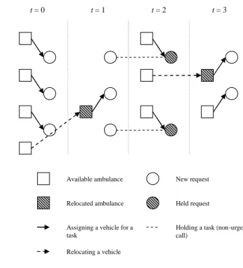
over the planning time horizon. Eq. (2) defines thevehicles in each location should be equal to total available resources, including newly available vehicles and also those which completed their tasks or relocated from the previous time periods. It is assumed that a vehicle, once it has finished its task, returns to the centre from which it is dispatched. Eq. (3) guarantees each task will not be serviced more than once, and Eq. (4) is the non-negativity constraint of the control variables. The model also allows a call to be rejected if it is in a lower priority and the number of available ambulances is low. Since our aim is to determine the assignment policy at t = 0, as the demand for t0 is forecast, a large T would produce a good enough approximation on a rolling horizon basis. An example with a horizon of three is illustrated in Fig. 1.
Each of the calls is associated with a priority or level of urgency. From the point of view of the dispatcher, the prioritization of calls can be weighted with the parameter ciat, which defines the reward for assigning a vehicle from i for servicing a task a at time t. A typical aim of a dispatching centre is to minimize the overall delay to all calls, and therefore an intuitive definition of the reward is a reward for handling a task related to its priority minus a function of the delay from i to j .a
t = 0 t = 1 t = 2 t = 3
Available ambulance
Relocated ambulance
New request
Held request
Assigning a vehicle for a task
Relocating a vehicle
Holding a task (non-urgent call)
Figure 1. A dynamic ambulance allocation and relocation model Let
a
q = the priority of task a, qa
1,2,3 aq
r = the reward for handling a task of priority qa
iat
h = the travel time from location i to location j to serve task a at time t, converted intoa
the unit of reward. We have
iat q iat r h c a , iI, a ,At tT (5)
Alternatively the model can be formulated as a recursive form, which will facilitate the analysis later on. Let Sit be the total number of vehicles to be available in location i at time t from all sources, and we have
k I t ki A a t ia it it R x iat y kit S , , (6)Define J to be the expected cost of a dispatching policy. The model can be specified recursively as follows
max 1
1
t t I i k I ikt ikt A a iat iat ,y x t t S c x d y J S J ikt iat (7) subject to it I k ikt A a iat y S x t
, iI (8) 1
I i iat x , aAt (9) 0 , ikt iat y x i,kI, aAt (10) where St ,
Sit iI
. A stochastic modelA stochastic model is also introduced to handle uncertainties in forecast demand. Randomness in the demand is introduced as probabilistic locations of a call arriving in the future. The framework takes the recursive form so that the recourse function can be approximated in various ways in the solution algorithm. Please refer to Wong et al. (2007) for the details.
SOLUTION METHODOLOGY
A possible approach in solving dynamic programming model is to calculate the recourse function explicitly for each state. However, computational complexity of the presented model is O
IS TJT
, and solving the model in practice is computational intractable. Algorithms for an approximate solution are usually used. An algorithm using the gradient approximation developed above is presented as follows.Step 0. Set a maximum number of iterations N, Set zˆitS,0 0 and zitS,00. Set n = 1 and t = 0.
Step 1. Forward pass. For the current n and t, solve the allocation and relocation
problem:
I i k I ikt n S t k ikt A a iat iat y x t k t S c x d z y J t ikt iat 1 , 1 , , max ~ (11) subject to it ikt iat y S x
, iI (12)1
I i iat x , aAt (13) 0 , ikt iat y x i,kI , aAt (14)Step 2. Once the xiat and yikt in Step 1 is determined, update St1; if t < T, then t = t + 1 and go back to Step 1. If t = T, go to Step 3.
Step 3. Backward calculation of gradients. For the current n and t, we update zˆitS,n
with zˆitS,n C
St,c1 C St,c2 , where C
St,c is the maximum total rewards of vehicle assignment, for given vehicle repositioning from the previous iteration and S for the current iteration. We can obtain left or right gradient attthe point of solution with c and1 c settings, which are vectors in the form of2
c i I
c ,i . If there are no vehicles repositioned to location i at time t-1, i.e. 0 1 ,
I k t kiy , zˆ stands for the additional benefit of having an extra vehicleitS,n
in location i at time t, and we have c1
0,,1,,0
with 1 for the ith element and 0 otherwise, and c2
0,,0
. If
, 10I
k t ki
y , zˆ is computed as theitS,n
negative consequences of removing a repositioned vehicle, by letting
0, ,0
1
c and c2
0, , 1,,0
with -1 for the ith element and 0 otherwise. C
St,c is obtained by solving the maximization problem:
I i a A iat iat x t t iat x c c S C , max (15) subject to i it A a iat S c x t
, iI (16) 1
I i iat x , aAt (17) 0 iat x iI , aAt (18) Step 4. Smoothing. Set zitS,nnzˆitS,n
1n zitS,n1.Step 5. If t > 0, then t = t - 1 and go back to Step 3.
Step 6. Terminate if n = N; otherwise set n = n + 1 and go to Step 1.
In Step 3 above, we can see that the value of zˆ will be large when the certain region oritS,n
whole of the system is busy in the next time period. However, zˆ is not larger than theitS,n
maximum setting of ciat in any case, because an actual call is more important than a predicted one of the same priority in the future. On the other hand, if the system is not busy and there are plenty of vehicles idle, the value of zˆ is diminishing. Step 4 adopts a stepsizeitS,n
is referred to as the smoothing constant. A typical choice of the stepsize is 1/n, a declining function with the iteration number.
EXPERIMENTAL RESULTS
To demonstrate the relative performance of the proposed methodology, a simulation model is setup to test against different scenarios. We will test the model against deterministic as well as stochastic settings of the problem. To capture the spatial manner of the ambulance dispatching, a network is created, in which nine potential demand zones and four medical centres are located in the network. Once there is a call to the dispatching centre, the dispatcher will assign ambulances from one of the medical centres for the call (or reject it). Travel time on each of the links is assumed to be one unit (5 minutes here), and therefore all potential locations are covered by a quickest response of 5 minutes. The corners are subject to less (but acceptable) coverage than those on the boundary or in the centre of the network. For the details of the setting of the problem, please see Wong et al. (2007).
Deterministic runs
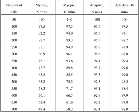
We first perform experiments on deterministic datasets. The dispatcher solves the whole period problem using forecast demand which is assumed to be deterministic. The gradients used in the adaptive algorithm are estimated from 50 training iterations. To eliminate the variation due to randomness, the evaluation of the solution in this section is computed from an average of 20 runs. Fig. 2 shows the total reward received in a simulation period against different demand intensity for myopic and adaptive strategies. Since the optimal solution is unknown to us, the reward is expressed as a percentage against the maximum possible reward received if no requests are rejected. The maximum possible reward is about linear to the number of requests. Both myopic and adaptive strategies reach 100%, i.e., the optimal solution, at a number of calls of 50. As the number of requests increases, the system is overloaded and not able to take up all the calls, and therefore the percentage of gain decreases, in which the rate of drop for the myopic strategy is steeper than that for the adaptive strategy. The adaptive strategy outperforms the myopic one by improving the overall efficiency. It is shown in Fig. 3 that the adaptive algorithm can consistently service more calls compared to myopic. This is probably due to the relocation of ambulances, which can save the travel times in the future operations. Table 2 displays the quality of services for Urgent calls, represented by a target of waiting period for the both strategies tested. We can roughly estimate the capacity of the medical system as 320 calls, which is an overestimation of 40 vehicles each taking maximum 8 tasks in 4 hours without idling. At the demand level of 300, 96.5% and 98.8% of Urgent calls can be reached within 5 minutes and 10 minutes respectively with the adaptive strategy. These percentages are 80.9% and 96.1% with the myopic algorithm. When the demand is increased to 600, with the adaptive strategy the percentage for urgent calls dropped slightly to 92.9% and 97.9%, in contrast to the heavy decline to 56.1% and 66.7% for the myopic one. This confirms the purpose of our dynamic model that suggests holding resources for future critical instances, without sacrificing too much the benefit of the current events.
0 10 20 30 40 50 60 70 80 90 100 0 100 200 300 400 500 600 700 800 Number of calls P e rc e n ta g e o f m a x im u m p o s s ib le re w a rd re c e iv e d Myopic Adaptive 0 10 20 30 40 50 60 70 80 90 100 0 100 200 300 400 500 600 700 800 Number of calls P e rc e n ta g e o f to ta l c a ll s s e rv e d Myopic Adaptive
Table 2. Target of waiting period of 5 minutes and 10 minutes for Urgent calls: Deterministic cases Number of calls Myopic, 5 mins Myopic, 10 mins Adaptive, 5 mins Adaptive, 10 mins 50 100 100 100 100 100 97.5 97.5 97.5 97.5 150 92.2 94.0 95.3 97.1 200 83.7 93.3 95.5 98.7 250 83.1 94.9 95.8 98.9 300 80.9 96.1 96.5 98.8 350 78.1 93.6 94.4 99.4 400 72.7 89.8 93.7 99.6 450 68.2 85.5 93.3 99.0 500 63.2 75.5 92.3 98.5 550 58.3 71.7 93.1 98.4 600 56.1 66.7 92.9 97.9 650 52.4 61.6 92.2 97.8 700 49.4 58.3 92.4 98.0 Stochastic Runs
We have also performed the numerical tests for Stochastic Runs in which there is uncertainty in the demand forecast. The sets of future tasks are given in probability and therefore unknown to the dispatcher at the time of making decisions. Due to the limit of spaces, the details on the the capability of the model in stochastic environment is discussed in Wong et al. (2007).
CONCLUSIONS AND SELF EVALUATION
Prioritization of requests is becoming a standard procedure in practice, and this paper is one of the first in trying to incorporate this component into the ambulance dispatch problem. In
Figure 2. Percentage of maximum possible reward received against the demand intensity: Deterministic cases
Figure 3. Percentage of total calls served against the demand intensity: Deterministic cases
the near-capacity situation, it is suggested that keeping or relocating vehicles to strategic locations could benefit the demand in the future. We formulate the problem with the objective of maximizing the reward gained for serving a request, showed as equivalent to minimizing the total delay incurred. The problem is formulated in a dynamic programming context, which suffersfrom the“curseofdimensionality”in applications of practical size. We propose a dynamic adaptive algorithm for solving the problem, approximating the gradient of the recursive subproblem in a linear form. Deterministic and stochastic settings of the problem are experimented with.Our model provides a guideline for accepting or not a current call with the computation of values of resources currently and in the future. Of course, rejected calls which are lower in priority would be kept track of by the operators for possible upgrading if needed. This model is particular useful in near-capacity conditions of dispatching, in which the tactical locations of medical centres and fleet of ambulances are already fixed.
REFERENCES
Andersson, T. and P. Varbrand (2006). Decision support tools for ambulance dispatch and relocation. Journal of the Operational Research Society, 1-7.
Ball, M.O. and L.F. Lin (1993). A reliability model applied to emergency service vehicle location. Operations Research, 41, 18-36.
Brotcorne, L., G. Laporte and F. Semet (2003). Ambulance location and relocation models.
European Journal of Operational Research, 147, 451-463.
Church, R. and C. ReVelle (1974). The maximal covering location problem. Papers of the
Regional Science Association, 32, 101-118.
Daskin, M. (1983). The maximal expected covering location model: formulation, properties, and heuristic solution. Transportation Science, 17, 48-70.
Galvao, R.D., F.Y. Chiyoshi and R. Morabito (2005). Towards unified formulations and extensions of two classical probabilistic location models. Computers & Operations
Research, 32, 15-33.
Gendreau, M., G. Laporte and F. Semet (1997). Solving an ambulance location model by tabu search. Location Science, 5(2), 75-88.
Gendreau, M., G. Laporte and F. Semet (2001). A dynamic model and parallel tabu search heuristic for real-time ambulance relocation, Parallel Computing, 27, 1641-1653. ReVelle, C. and K. Hogan (1989). The maximum availability location problem.
Transportation Science, 23, 192-200.
Thakore, S., E.A. McGugan and W. Morrison (2002). Emergency ambulance dispatch: is there a case for triage? Journal of the Royal Society of Medicine, 95(3): 126-129. Toregas, C., R. Swain, C. ReVelle and L. Bergman (1971). The location of emergency service
facilities. Operations Research, 19, 1363-1373.
Wong K.I., Kurauchi Fumitaka and Bell M.G.H. (2007). On-line ambulance dispatching heuristics with the consideration of triage. In R.E. Allsop, M.G.H. Bell and B.G. Heydecker (ed.) Transportation and Traffic Theory 2007, pp 461-481. (ISBN 978-0080453750)