A study of the Kuroshio's seasonal variabilities using an altimetric gravimetric geoid and TOPEX/POSEIDON altimeter data

JOURNAL OF GEOPHYSICAL RESEARCH, VOL. 101, NO. C3, PAGES 6313-6335, MARCH 15, 1996

A study of the Kuroshio's seasonal variabilities using

an altimetric-gravimetric

geoid and

TOPEX/POSEIDON

altimeter data

Cheinway Hwang

Department of Civil Engineering, National Chiao Tung University, Hsinchu, Taiwan

Abstract. The first year of TOPEX/POSEIDON (T/P) altimeter data were used

between

the T/P and gauge

sea levels at selected

tide gauge

stations

around Taiwan

deep ocean and both show an annual cycle with an amplitude of 15 cm. A 3' x 3'

and T/P altimetry. To account

for the oceanographic

signal in the altimeter data,

(SST) based on a global averaging

concept

and a spherical

harmonic expansion

cm. The SST values derived from the geoid and the data along T/P's descending

variability of all quantities is 25%. All the variabilities are relatively large near the

Introduction

In east Asia the Kuroshio Current, one of the western

boundary currents, plays a key role on the local fishery, navigation, and circulation [Tang and Yang, 1993]. The Kuroshio is part of the circulation system of the West- ern Pacific Ocean. The Kuroshio begins at the east coast of Philippines; after leaving the northeast coast of Taiwan, it follows roughly the 200-m isobath before it reaches south of Japan [Hu and Chang, 1992]. In comparison to the Gulf Stream, which was extensively studied with satellite altimetry [e.g., Tat, 1990; Zlot-

nicki, 1991; Rapp and Smith, 1994], the Kuroshio

did

not receive

the same attention with altimetry. (Note

that researchers

like Tat [1990]

and Zlotnicki

[1991]

fo-

cused

only on the Kuroshio

Extension). The reason

Copyright 1996 by the American Geophysical Union. Paper nmnber 95JC03800.

0148-0227/96/95JC-03800505.00

the lack of a good geoid or the lack of confidence in the altimeter data quality over this area, especially for data from Seasat and Geosat. In fact, the geoid plays a

crucial role in extracting oceanographic signals over the

western boundary currents such as the Gulf Stream and

the Kuroshio [Rapp and Smith, 1994]. Over the Gulf Stream area several geoid models exist, e.g., the models of Marsh and Chang [1978], Wessel and Watts [1988], and Porter et al. [1992]. Recently, Rapp and Wang [1994] developed a geoid model for the Gulf Stream using marine gravity data and the model was used in a study of the Gulf Stream characteristics [Rapp and Smith, 1994]. However, little attention is paid to the construction of a detailed geoid over the Kuroshio, al- though such works do exist, e.g., Fukuda's altimetric- gravimetric geoid cited by Segawa [1991, p. 128]. In fact, the Kuroshio travels through a much more com- plex gravity field than the Gulf Stream area, so the need

of a high-resolution geoid for the Kuroshio is more criti-

cal than the Gulf Stream. Thus, in this study, one of the primary goals is to construct a detailed local geoid us- ing existing altimeter data and gravity data. Altimeter 6313

6314 HWANG: KUROSHIO'S VARIABILITY USING GEOID AND TOPEX/POSEIDON

data will be used because with the sparse gravity data alone (see below), there will be no possibility of getting

a high-resolution geoid. However, altimeter data con-

tain gravity signals as well as the oceanographic signals,

which must be carefully taken into account when com-

puting the geoid. Such an altimetric-gravimetric geoid

should fulfill the requirements that it can not only be

used for determining the short wavelength signals such

as the fronts of the Kuroshio but also for identifying the

long wavelength features such as the general circulation

of the Western Pacific. With a precision geoid, the next goal of this study is then to quantify the seasonal vari- abilities of the Kuroshio from the TOPEX/POSEIDON (T/P) data.

In the context of this study the Western Pacific is de-

fined to be within 105øE- 140øE and 5øN - 35øN and the Kuroshio Extension will not be covered. It is known

that the primary goal of the T/P mission has been to

determine the general circulation of the oceans [Fu ½! al., 1994]. For a study of this kind a global data set is prepared, and normally the data over shallow seas

are excluded. One of the reasons for data exclusion over shallow seas is due to the uncertainty in the ocean

tide model. On the other hand, Mazzega and Berg• [1994] have computed the major tidal components in the Asia semiclosed Seas [such as the South China Sea and the Japan Sea] and obtained promising results, im- plying that the T/P altimeter system (including the

orbit, geophysical corrections, and other factors affect-

ing the measured sea surface height) over shallow seas

should function very well except for the tide models.

Furthermore, when doing intercomparison between the T/P sea level and tide gauge sea level, researchers tend to select the gauge stations in the deep ocean, and it has not been shown whether the comparison over shal- low seas will yield the same good agreement as for the deep ocean. For scientists who pay more attention to a local area than the entire globe these are the questions they often raise and they are keen to know the answers, especially when the studied area has a possibly unfa- vorable condition for the T/P altimeter system. Thus we will first investigate the performance of the T/P al- timeter system over the studied area using tide gauge

measurements. We will focus on both the numerical

technique of geoid computation and the analysis of the sea surface topography (SST) regarding the character-

istics of the Kuroshio and the Western Pacific.

TOPEX/POSEIDON

Data Processing

and Averaging

The T/P data used in this study were supplied by Archiving, Validation, and Interpretation of Satellite Data in Oceanography (A VISO) [1992]. It is the sea sur- face height (SSH) above the reference ellipsoid that will be used in our analyses. In order to obtain reliable SSH, the criteria used by Denker [1990] were employed to edit the Geophysical Data Records (GDRs). After passing

the editing criteria, geophysical corrections were applied

to the instantaneous SSHs. In other altimeter missions

such as Seasat and Geosat, the accuracy of satellite or- bit has been a primary error source for SSH . However, the 5-cm radial orbit accuracy of T/P [Tapley et al., 1994a] is now comparable to the errors of geophysical corrections. In particular, we expect the error in ocean

tide model at the vicinity of continental shelf or shal-

low seas will probably exceed the T/P orbit error. For a geophysical correction the T/P GDRs contain various

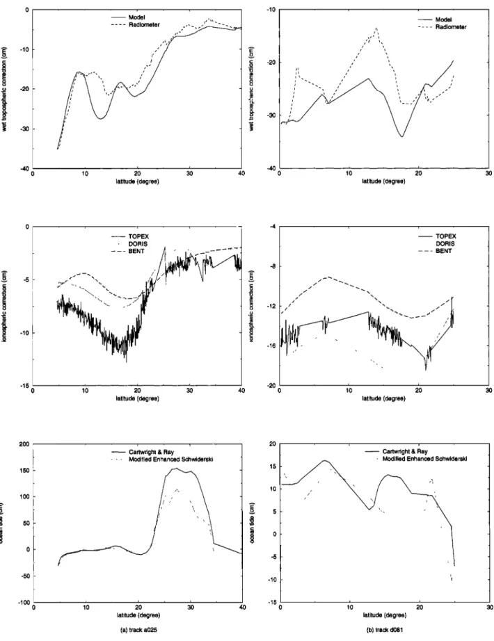
models for use. Figure 1 compares the various models of

ionospheric correction, wet tropospheric correction, and ocean tide along arcs a025 and d081 of cycle 18. These two arcs, whose ground tracks are plotted in Figure 2, travel from the deep ocean to shallow seas and from the tropic to the high latitude. Arcs a025 and d081 corre- spond to passes 51 and 164 defined by A VISO [1992]. The symbol "a" stands for "ascending," and "d" is for

"descending." This convention will also be used in other

figures of this paper. The formula for conversion be- tween arc and pass is pass: 2 arc+ 1 for an ascending arc, and pass = 2 (arc + 1) for a descending arc. We notice from Figure I that south of 20øN the difference in ionospheric correction between the T/P model and Doppler orbitography and radio positioning integrated by satellite (DORIS) model is about 5 cm, which is the size of the T/P radial orbit error. Since the T/P iono-

spheric model is direct from the dual-frequency mea-

surements and has accuracy of the order of 1 cm [Imel, 1994], it is selected for correcting the TOPEX range measurements; for the POSEIDON measurements, the

DORIS ionospheric model is adopted because the result

from Escudier et al. [1993] has shown that it provides

sufficient accuracy for a single-frequency altimeter. The

root mean squared (rms) difference of the two wet tro- pospheric models is also about 5 cm, and the difference is particularly large in the tropical area. The radiome- ter model was adopted for the wet tropospheric cor- rection. As far as the ocean tides are concerned, the Cartwright and Ray model and the modified enhanced

Schwiderski agree quite well in the open ocean, but the

two have large differences over shallow seas, reaching 30

cm. Many studies, e.g., Eanes el al. [1993], have con- firmed that the Cartwright and Ray model has a better

accuracy than the modified enhanced Schwiderski; thus

the former was used in this study. Recent works by, e.g., Ma el al. [1994], Schrama and Ray [1994], and Knudsen [1994], have improved the Cartwright and Ray model by 1-2 cm, and we expect that the application of these new tide models to the T/P GDR will improve our analysis. A note is given to the correction due to different flat- tenings of the reference ellipsoids used by TOPEX'and POSEIDON. The correction is [Rapp, 1989]

Ah

- aAf(1

- f)sin

2

qb

(1)

where Af=1/298.257- 1/298.25653577, W =

/1

- (2f

- f2

sin

2

qb),

and

a,

f, qb

are

the

equatorial

ra-

dius (6378136.3 m), flattening, and latitude, respec- tively. Here Ah increases from zero at the equator to

HWANG: KUROSHIO'S VARIABILITY USING GEOID AND TOPEX/POSEIDON 6315 -lO -20 -30 -40 , . Model Radiometer latitude (degree) -10 -20 -30 -40 ! ! ! -- Model .... Radiometer latitude (degree) 0 -15 0 -- TOPEX ... DORIS BENT ß ;,_,%. ',, 10 2•0 30 latitude (degree) -- TOPEX --DORIS BENT -8 jjJ -12, •/ _.-,. "%, _•_•.jjJ -16 -20 ' • ' 0 10 2•0 latitude (degree) 200 150 100 50 •- -100, 0

Cartwright & Ray ... Modified Enhanced Schwiderski

-lO

-15

• Cartwright & Ray

erski

ß

' •'o ' •'o ' •'o ' •o o ' •'o ' io

latitude (degree) latitude (degree)

(a) track a025 (b) track d081

Figure 1. Comparison of various models of geophysical corrections in the TOPEX/POSEIDON

Geophysical Data Records for track d081 and track a025. For the ionospheric corrections, the

6316 HWANG: KUROSHIO'S VARIABILITY USING GEOID AND TOPEX/POSEIDON 117 ø 118 ø 119 ø 120 ø 28 ø 27 ø 26 ø 25 ø 24 ø 23 ø 22 ø 21 ø China 121 ø 122 ø 123 ø 124 ø / :28 ø ß ß ß ß ß

,,,," , •';,/'

27 ø

,

,,

.,:::.•,•

26 ø

'::!,:--..

....

?:,..

, .:_

,-

'-•Oob..'_•

24"

!?:---

-',,_. ...

;, • ",':;

_{', %•o0o}

,,'

,,'_, ",,,,

_o

_o

_{21 ø}

'i;,'!,,"!"i

'"'---:,

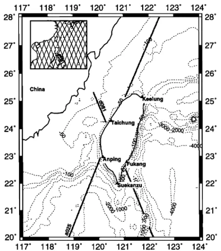
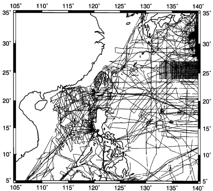
Figure 2. Distribution of selected tide gauge stations for T/P sea level comparison; also shown are T/P tracks a025 and d081. The contours (dashed lines) are bathymetry at selected depths. The inserted map shows all the T/P ground tracks over 105øE- 140øE and 5øN - 35øN.

SEIDON's SSH in order to make the two height systems consistent.

For later development the SSH from the first 36 cycles

are averaged according to seasons, and a final averaging

is made for one year. The relationship among the first

36 repeat cycles, dates, and the four seasons is given

in Table 1. Because of the highly accurate orbit, the T/P SSH were not subject to orbit adjustment, which is the common practice for data from other satellite mis- sions. Also, the adjustment of the T/P orbit may have

the possibility of removing oceanographic signals. Note

that Tai and Kuhn [1994] have adjusted the T/P altime- ter data and obtained improved orbits. The averaging

cannot remove the geographically correlated orbit error

(if any) and nonperiodic time-varying errors introduced

by the geophysical corrections. The averaging certainly

Table 1. Relationship Among the First 36 Repeat Cy- cles, the Dates, and the Four Seasons

Cycles Dates Season

1-9 Sept. 22, 1992 to Dec. 21, 1993 fall 10-18 Dec. 22, 1993 to March 21, 1993 winter 19-27 March 22, 1993 to June 21, 1993 spring 28-36 June 22, 1993 to Sept. 21, 1993 summer

can reduce the random errors due to the altimeter itself

and the instruments for obtaining geophysical correc-

tion models. The averaging can also reduce the periodic

time-varying errors if the period of averaging happens to coincide with or is close to the integral multiple of the period of the error. For example, all the major ocean tide components have periods less than I month, and the 3-month averaging period for a season should reduce the major tidal errors.

Verification of the TOPEX/POSEIDON

System Using Tide Gauge Data

To evaluate the T/P altimeter system over the Kuros-

hio, we compare the monthly sea level as measured by

T/P and by tide gauges at five selected tide gauge sta- tions around Taiwan (Figure 2). The stations Keelung and Fukang are at the immediate vicinity of the deep

ocean, and the rest lie on the shallow seas west of Tai-

wan. Note that the mean sea level at Keelung is the

vertical datum of Taiwan. Since we are interested in

the seasonal variation of of the sea level, the gauge data

were averaged monthly to remove the ocean tide effect. To obtain the monthly T/P sea levels, for each repeat cycle we first construct a 10 x 10 grid from the along-

HWANG: KUROSHIO'S VARIABILITY USING GEOID AND TOPEX/POSEIDON 6317

Table 2. Correlation Coefficients Between

TOPEX/POSEIDON and Gauge Sea Levels

Gauge Station Coefficients

Keelung 0.828

Taichung 0.541

Anping 0.482

Suekanzu 0.734

Fukang 0.909

track SSH using a minimum. curvature fitting [Wessel and Smith, 1991] for an area covering all the stations.

Three such grids from three consecutive cycles are av-

eraged to yield a monthly grid. The sea level at a de- sired tide gauge station is then obtained by interpola-

tion. This method does not work well for the station

Fukang, so for this particular station we decided to get the monthly sea level by averaging all the SSH within

100 km of the station. Table 2 shows •he correlation co-

efficients between the T/P and gauge sea levels. From

Table 2 we see that the two sea levels which are at the

boundary of the deep ocean have a high correlation at the east coast of Taiwan. Over shallow seas the perfor- mance of the T/P altimeter system is only fair as in-

dicated by the low correlation coefficients there, which

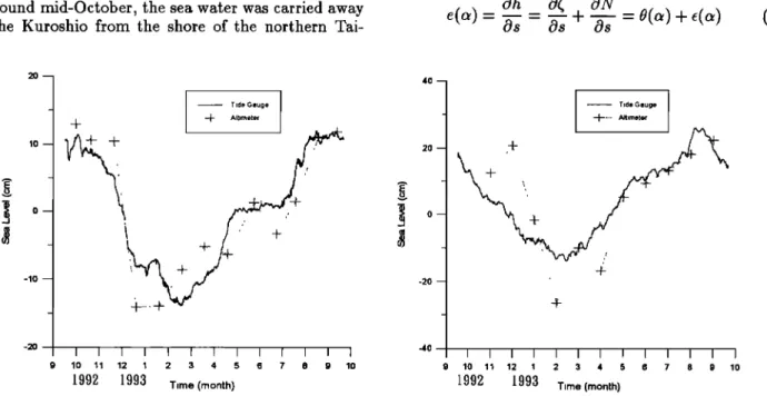
are probably due to tide model errors. Figure 3 shows the monthly sea levels from T/P and tide gauges at Keelung and Fukang, where the correlation coefficients are 0.828 and 0.909, respectively. Both the T/P and the gauge sea levels appear as a cosine function with a 1-year period. The zero phase (or the highest sea level) occurs in August, and the amplitude is about 15 cm. According to Tang and Yang [1993], the rise and fall of the sea level at Keelung are strongly correlated

with the activity of the Kuroshio. As the Kuroshio "in- trudes" into the continental shelf of the East China Sea

in around mid-October, the sea water was carried away by the Kuroshio from the shore of the northern Tai-

wan, causing the sea level at Keelung to descend. The

"intrusion," as well as the decrease of the sea level at

Keelung, continues all the way to March. From March, the Kuroshio gains its strength gradually by perhaps the heating in the tropic, and it begins to move toward the deep ocean (i.e., to the east). The accompanying rise of the sea level at Keelung beginning in March is due to in part the cease of the "intrusion" and in part the overall increase of the water mass carried by the

Kuroshio. The implication of this comparison is that

the T/P altimeter system may perform very well even at the vicinity of the deep ocean.

An Altimetric-Gravimetric Geoid Over

the Western Pacific The Method

The method we will use to construct a local geoid for

the Western

Pacific

is least squares

collocation

(LSC)

[Moritz, 1980], which is the only known

geodetic

tech-

nique in using heterogeneous data. First, we will dis-

cuss the altimeter data type to be used. The altimeter- measured sea surface heights contain both geodetic and oceanographic signals and measuring errors. Except for T/P, the data errors have largely come from the satel-

lite's

drbit. Considering

all these

effects,

an altimetric

SSH, not including the random noise, may be expressed

as

where ( is the SST, N is the geoidal height, and b is the orbit error, which is assumed to be a constant within a arc of less than, say, 4000 km. To avoid the error b, we may use the along-track sea surface gradient (SSG) obtained by Oh ch• ON

-

-

+ W - 0(.) +

(3)

"'

I: ,:,•_.•_,/":•

Figure 3. Comparison

of sea levels

measured

by tide gauges

and by T/P altimeter

at (left)

6318 HWANG: KUROSHIO'S VARIABILITY USING GEOID AND TOPEX/POSEIDON where a is the azimuth of the track which may be cal-

culated by an approximate formula by Hwang and Par-

sons [1995]. Note that the azimuth varies along the

track. Thus a SSG contains both the SST gradient and the geoid gradient which is a functional of the Earth's gravity field. Another type of data related to the geoid is gravity anomaly. With SSG and gravity anomalies as

data, we:ckn

use LSC to predict

geoidal

heights.

To this

end we•

.•i:ll have

to'determine

the required

covariance

ent are uncorrelated, the covariance function of SSG is

the sum of the covariance functions of geoid and SST

gradients' •

:"

C** - Co..

+ C•

(4)

The covariance

function

of'geoid

gradient C• has been

derived

by Hwang

and.

Par{on•

[1995]

(Appendix

A).

The

cøvariance

functiOh

o,f

$ST

gradient

Co

may

be

de-

rived:Using

the 'Proce,d:qr

'e•

of Moritz

[1972]

and Moritz

[1980].

First, we expand;the

SST into a series

of spher-

ß

K n

+

sin

n--O m=O

P,•.,

(sin

•))

(5)

where

•b and A are latitude and longitude,

P•r• is the

fully normalized associated Legendre function of degree

n and order m, and K is the maximum expansion de-

gree. Using the analogy in deriving the covariance func-

tion of the Earth's disturbing potential, the global co-

variance function of SST is

cc(•)

= •4 It(0, x)C(0', x')]

=

((•, •)((•' •').

8•2 =0 a •=-•/2 =0

'

= • c• v• (•os

•)

(•)

where M is the global averaging operator, • is the spherical distance, P• is the Legendre polynomial, and (• is the degree variance of the SST defined •

anm

q- bnm

)

(7)

m--O

With the covariance function of SST we can then deter-

mine the covariance function of SST gradient using the

law of covariance propagation [Moritz, 1980]. First, we

have to determine the isotropic covariance functions of

SST gradient. Using the method of Moritz [1972] and Tscherning and Rapp [1974], the covariance functions

of the longitudinal and transverse components of SST

gradient, which are isotropic, are

C• -- (tC'½

-sin

2 •bC';)/R

2

where t - cos •p and R - 6371 km is the Earth's mean

radius. Using (6) we have

K • d •

C½(t)

= d-•[C½(t)]

-- E (nPn(t)

=

n(• 1 - t

-

d2

K

C½

(t) =dt 2[C½(t)]

- E (nPn

(t)

(1

-t2)

2P•-•(t)

_ (1

- n)t

2 + n + 1

Pn

(t)]

In the above two equations the differential relationships

of Legendre's polynomial [Lebedev, 1972] have been em-

ployed. Note that when t - 4-1, singularities will occur

and they are treated in Appendix A. Following the pro- cedure of Hwang and Parsons [1995] for deriving the covariance function of geoid gradient, the covariance function between a SST gradient at P with azimuth ap and a SST gradient at Q with azimuth aQ is

co(P,

Q) -

C•r• sin(ap

-- aeQ)

sin(aQ

- aeQ) (12)

where apQ is the azimuth from P to Q. Furthermore, the covariance of geoid gradient has exactly the same form as Co(P, Q)[Hwang and Parsons, 1995]'

c•(P. Q) - c[• •o•(.• - .•)•os(.o

- .•)+

C•r • sin(ap -- CtpQ)

sin(ctQ

- apQ) (13)

longitudinal and transverse components of geoid gradi-

ent. Thus the covariance function of SSG is

c** - (c• + c/,)•o•(.•. - .•.•)•os(.• - •.•)+

(c•,• + C•r•) sin(o•p

-- o•Vq)

sin(aq

-- o•Vq)

(14)

Other required covariance functions are those for

geoid-SSG, gravity anomaly-SSG, geoid-gravity anomaly,

and gravity anomaly-gravity anomaly. Assuming zero correlation between the Earth's gravity field and and

the SST, the covariance function for geoid-SSG is

cov(N,

e) - cov(N,

e) - Cn• - - cos(aq

- O•pQ)CiN

and the covariance function for gravity anomaly-SSG is

cov(Ag,

e) -- cov(Ag,

e) -- Cag• - - cos(o•Q-O•pQ)ClAg

HWANG: KUROSHIO'S VARIABILITY USING GEOID AND TOPEX/POSEIDON 6319 geoidal height and gravity anomaly, respectively. Equa-

tion (15) and (16) are again

based

on the derivations

by

Hwang

and

Parsons

[1995].

In this

study,

except

C• and

C•mm,

all other required

isotropic

covariance

functions

Tscherning and Rapp [1974].

The degree variances in (7) were determined using a

spherical

harmonic

expansion

of the Levitus

SST [Lev-

of the Levitus SST; see also the discussion by Engelis

[1987]. In the spherical

harmonic

expansion,

the SST

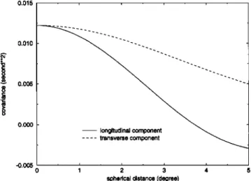
land values are assumed to be zero. Figure 4 shows

the two isotropic covariance functions of SST gradient,

which have low variances and large correlation lengths

due to the long wavelength nature of the Levitus SST. In the practical use of LSC, we employed the so-called remove/restore procedure with the Ohio State Univer-

sity 1991

gravity model

(OSU91A)

to degree

360 [Rapp

covariance functions are computed using the error esti-

mates of OSU91A coefficients in a Legendre polynomial

series

[Hwang

and Parsons,

1995]. A LSC computation

is carried out in a 0.250 x 0.250 inversion cell with a data border of 0.60 ø which is selected based on numerous tests. This choice of cell size and data border requires

least computational time, and the large ratio between

the data border and the cell size has ensured a smooth

transition of the predicted geoidal heights between two adjacent cells. Furthermore, because the LSC computa-

tions are made locally, all the covariance functions men-

tioned above must be scaled to reflect the local behav-

iors of the covariance functions. For the prediction for- mulae, use of covariance functions in the remove/restore procedure, and use of scaling factors, see Appendix B and the work of Hwang and Parsons [1995].

The Data and the Result

Using

the method

of LSC, we have

computed

a 3 • x 3 •

percomputer.

Due to the enormous

amount of data,

a total of 29 CPU hours is consumed. The SSG used

are from Seasat,

Geosat/Exact

Repeat

Mission

(ERM),

points

in a 10 x 10 cell. The ERS 1/GM includes

data

from the first 168 days of the geodetic mission and has

a very dense data distribution. However, the accuracy

of ERS 1/GM is the poorest

among

all data. The ERS

T/P data are based

on the first 36 cycles

average.

All

ror variances

form the diagonal

elements

of De in (B5).

The error variances of the SSG are obtained by the sim- ple statistics that use the repeat measurements on the

same location. It is clear that an "error variance" com-

puted in such a manner contains both the white noise spectrum and the variability of the sea surface. Thus the error variances may not have the desired normal distribution. However, a SSH with a high variability,

0.015 0.010 0.005 0.000 -0.005 0 1 2 3 4 5

spherical distance (degree)

Figure 4. Covariance functions of the longitudinal and

transverse components of sea surface topography (SST) gradient. Both have relatively long correlation lengths, due to the long wavelength nature of the SST.

and hence a large error variance, will yield a less reli- able mean SSH over a limited time span of averaging. Therefore an observation with a large error variance will

be less weighted, and this is precisely what we want in

the LSC computations. Seasat and ERS 1/GM do not

have repeat measurements so we assign a uniform stan-

dard deviation

of 10 /•rads for the

m, based

on the es-

timated 5-cm noise of range measurement and 6.73-km

along-track distance [Hwang and Parsons, 1995]. The gravity anomalies used contain data both on land and on sea. Figure 5 shows the data distribu- tion. In fact, for the land values, only data over Tai- wan, which are collected by Yen et al. [1990] in a 7-year

campaign, are used. The marine gravity anomalies are

from the National Geophysical Data Center (NGDC) database, and the data density is low along the path of the Kuroshio. The sparsity justifies the need of high- density altimeter data. The quality of marine gravity varies from one cruise to another, but its White noise is believed to be well below i mgal [Hwang and Parsons,

1995]. For the LSC computations it is decided to as- sign an uniform standard deviation of I mgal for all the

gravity data. The land gravity anomalies over Taiwan

are important for the determination of the Kuroshio's variability east of Taiwan. This is because near coastal areas, altimeter data are edited out; the use of land data will help to increase the resolution and accuracy of the predicted geoid there. Furthermore, terrain cor- rections for the land gravity anomalies, computed us-

ing the fast Fourier

transform

technique

described

b•

,

30"

Schwarz et al. [1990] are applied using a x 30 digital terrain model. Due to the rugged terrain over Taiwan, the maximum terrain correction is 70 mgals

with a mean and a standard deviation of 2.2 and 5.3

mgals, respectively. As given by Hwang and Parsons [1995], the marine gravity anomalies are adjusted by a quadratic polynomial with respect to the satellite grav- ity anomalies derived from Seasat, Geosat/ERM, ERS i 35-day, and T/P data.

6320 HWANG: KUROSHIO'S VARIABILITY USING GEOID AND TOPEX/POSEIDON

105 ø

110 ø

115 ø

120 ø

125 ø

130 ø

135 ø

30 ø

20 ø

15 ø

10 ø

105 ø

110 ø

115 ø

120 ø

125 ø

130 ø

135 ø

Taiwan are available.

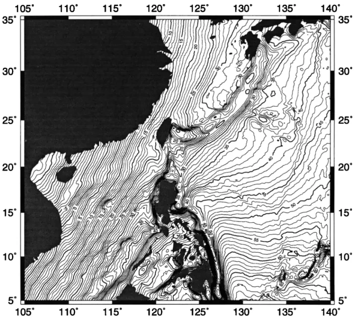
Figure 6 shows the predicted marine geoid over the

Western

Pacific. This local geoid

clearly

reveals

the

high-frequency tectonic structures, e.g., the Philippine

Trench, the Ryukyu Trench, and the Ryukyu Islands. Since the Kuroshio travels through the Philippine Tre- nch, the east coast of Taiwan, and the boundary of •he Ryukyu Islands, one would need such a high-resolution geoid to identify its fronts as its width could be well

below 100 km; see also the development below. Figure

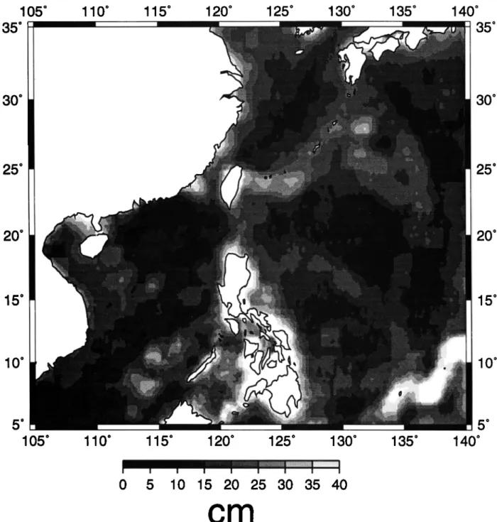
7 shows the error estimates of this local geoid. From Figure 5 to Figure 7, two points may be concluded: (1) the use of marine gravity anomalies will reduce the geoid error, and, in general, the geoid error is below 5 cm in the presence of highly dense gravity anomalies, e.g., the spots near 25øN, 140øE, and 20øN, 115øE; and (2) in the areas of high-frequency geoid variation, e.g., the trench areas and islands, the error is large. Special attention must be given to the geoid error along the

Kuroshio's path. From Figure 7, the geoid error along

its path varies from the minimum of 15 cm near the 200-

m isobath to the maximum of 35 cm near the east coast

of Taiwan. The fact that the predicted geoid is subject

to errors indicates that the true resolution may not be

3' x 3' and the predicted geoid should be filtered in some way before use. We finally note that the error of the predicted geoid is much less than the 49-cm commission error of the geoid from OSU91A to degree 360 [Rapp,

Seasonal Variability of the Kuroshio

uses. One of the uses is to study the seasonal variability

of the Kuroshio. First, we will investigate the "shape"

of the SST across the Kuroshio front and determine the

parameters of interest (see Figure 6.23 and Table 6-1 of

HWANG: KUROSHIO'S VARIABILITY USING GEOID AND TOPEX/POSEIDON 6321

105 ø

110 ø

115 ø

120 ø

125 ø

130 ø

135 ø

140 ø

35 ø

35 ø

105 ø

110 ø

115 ø

120 ø

125 ø

130 ø

135 ø

140 ø

Figure 6. The predicted altimetric-gravimetric geoid over the Western Pacific; contour interval

is lm.

boundary current). Following the works by Zlotnicki [1991] and Rapp and Smith [1994], the along-track SST

across the Kuroshio front can be approximated by the hyperbolic function:

((x) - Htanh(

_ß

x- x0

_{L )+(o}

₍₁₇₎

where the parameters to be determined are [Rapp and Smith, 1994] H, 2H is the height jump, which will be

denoted as A• 7 below; x0, which corresponds to the lo-

cation where the maximum geostrophic velocity occurs (see below); L, 1.89L is the along-track width of the

Kuroshio; and (0, an unknown constant.

Note that one can also use the error function for ap-

proximating the SST, as given by Tai [1990] and Rapp and Smith [1994]. The along-track width of 1.89L is based on the 45.6 % falloff of the velocity at the edge of the Kuroshio [Rapp and Smith, 1994, p. 24,709]. The

along-track distance x increases in the satellite's flight

direction. By this definition a positive velocity will be to the left when viewing toward the positive x direc- tion. The height jump may be used to estimate the baroclinic transport with a two layer approximation as suggested by Tai [1990]; see also Zlotnicki [1993]. By that approximation, for a mean thermocline depth of 500 m the relationship between height jump (AT) and baroclinic transport at midlatitudes is

baroclinic transport- 50A•? (18)

where the unit for baroclinic transport is 106 m 3 s -•

(Sv) and the unit for At/is meters.

Thus by (18), 1-m

height jump corresponds to 50-Sv baroclinic transport.

The problem of determining the four parameters is nonlinear, and we use the following procedure to find the solution'

1. Determine the maximum geostrophic velocity and

x0. With the geostrophic equation the velocity field corresponding to the SST function in (17) is

6322 HWANG: KUROSHIO'S VARIABILITY USING GEOID AND TOPEX/POSEIDON

105 ø

110 ø

115 ø

120 ø

125 ø

130 ø

135 ø

140 ø

•::•i

f:::i:.

i;::•

}":.

::'i:

:::::::::::::::::::::::::::::::::::::::::::::::::::::::::::::::::::::::::::::

!::;:.•.::

;}[;i:'

- ..ii:i.:"

...

.5:::

:•

}•-

.'..!

•

•

::

::

i:.5::

::?:

i

i

::;•::

::!i

::•:::.!

::

!::*.•

:.;

i::C::}iC;:

::

I

-

.<•'•'-•-..':...-•::.:c"•

::.:•.;>:..::,.:-•:.:.:::-:.:<•,•?"",-

-."-•:-'..

-. •:•:'•-;.<e.'..•i•::•::•::•i•:::i•::•::•:•

".:-'-":'-'

:•;ii:::::::!i•!•:•;•:::.:..:.•'"•½•'.•½::i:::::::::::i::•::

...

::::::::::::::::::::::::::::::::::::::::::::::

ß 25 ø

ß ..""?!•5:i•..>..•.•.•..•... .:,5:::;:Ii:::!:•½[ .::i::•: ::?" '•••••••... '"'"" ' '" •' '• -•:.'-'• .... *:•i•:::•::::::•i•ii::::::::i:::: ::::::::::::::::::::::::::::::::::::::::::::::::::::::::::::::::::::: ß

ß

•:

...

•:":'":•i•i.

&•...

:• :.:.,.'•:::::•::•i•?:::::::::::::::::::::::

...

•i:i•

•i•

•::•::•::'•:i•i•::•

•::•:•::•

•::•

•i•

:.

.•::::-.::::...•':•:•i!',}i';•::.

?' :::::?,i:

'?:i:i;•iiiii•:-.-."•ii',:.i:•;',::.

:::::

...

:,•,:

.

:.. •:!i i::::• .. 5::; ;::[ !;:: •;•-:½::!: ' ":! •:'" ..[•;: :i:i:::!::i • •.ii • .:.•-x.:)i..!•: :::i;iS. .'i•i:..:[ {ii[i ';:!!i" .

' . '•:: •:::}::..,, .:•:!i•ii:!:i:•iii!i!!ii!!!i• :i .. :i::'.•!'.": ... !!:.... "•:½•:.!•:!:•::!::::;:!i ... !•!::!•!::•! ... •i::•::•

... ;:i'::•.::•.: •:!i•!•i:i•z!:•::i!iiii::!!:i•i ' .::.!i•. :: ::: :::.:.:! .... ':: •"- .!..•ii!!. •'. :'":'"•:i?..•:i:i.. ':i ::!::i!: i :!i!! •i.•!!!:!•!i!:

'::•" ;::::' ... -:•' ,.:.:•i :> ...::... '•>. '•:•{ii::. .:i'• i!!i. '.':-•:: !2:!!.;::::•::i:•. :i!!i!!::. :!' :: .2:!..::!:: ... " .::: ½ 3 :[:::i::½i::'::i:L.:. ' [:i". :'"" -.:: :::2

... •:½:;..•½:"ig•.iii';...•!•.,•?i:•:•;" :½:'•'::;:.'::•:::.%•:.'"i!.,..:' ... ":•:..• :'.,-.½•:: • ? '•!¾ .:•::i::i•.:,:'•:).i;iiii!ii•.. ß ::::::::::::::::::::::::::::::::::: •;:::::::•:•i•::iii•i•!:?i'"•?:.•i•!•:•:::•::::::::::•::C •::::.-:•.;• ... . •

... ' ... '"' :.',: .... •::...:.'-:::::!•:•i.' i:!•i!•,:!7!½:.:'•..,'-.".':•5iC ,'<....,..:..[i•.:....':,i. i::i-':ii' :'4i:iii[i!i[:ii:::}:::':' . .:.::.,>. igi..:i!iiii:i:!!i•':..: .:.7."•.•.-::.'-.::.:½5:5-!-'z:=7.-: .':' .... -•' .--"

•'•:."• ... . ... ' •'-'.'• ... :•::•.: .:•: ,'::---:•:'"'•:::.:•-•.'•--: ": ... '::•.• ':•.-: ::?':fi•'•ii;-::•::i: :.:•.'".":'::' • •i!• i: :i:::• -'½' ... •:•:•:•::•:i':•i:' ':•:. •

5 o ß

. ":•

':..:¾.x'?:...:.

...

::::"

"'"::•:'•:•:"•;'?;•"•

•" '":'•

... '::'"" ' "':•:•:"'""::•:•'"'":•'•'::'"•::'

...

:': '::::•:•'•;;•:"•:•i•i•::•:•::•::•:•l

5 o

105 ø

110 ø

115 ø

120 ø

125 ø

130 ø

135 ø

140 ø

0 5 10 15 20 25 30 35 40

cm

•'igure 7'. A gray-shaded map of the error estimates of the altimetric-gravimetric geoid (see

Figure 6). Errors over land or larger than 40 cm are masked with white.

v(x)- g (9•

_fOx-fL

_ gHsech2(X-xo

_{L )}

₍₁₉₎

where g is the normal gravity and f - 2f•sin•b with • being the Earth's rotational velocity (7.292115 x

10-•rads

-1). The maximum

velocity

occurs

at x - x0

gH

v.• = f •

(•o)

Therefore we first smooth the SST data using a filter, and then use numerical differentiation to find and v(x). Among all the velocity values, there exists a

maximum which is the desired Vm• and the correspond-

ing x is x0. From x0 we then calculate the location of

v,•, which can be viewed as the axis of the Kuroshio.

Once Vm• is found, (20) becomes a condition which the parameters H and L must satisfy, so now we are left with only two parameters to estimate: H (or L) and (0. 2. Find H and (0 by linearization and iterations. For the remaining parameters H and (•0 we may form the

observation equation for a filtered SST value as

(+ v½-

Htanh

[fv,•,(x-x0)]

+ (0 (21)

HWANG: KUROSHIO'S VARIABILITY USING GEOID AND TOPEX/POSEIDON 6323

ear model of (21) can be linearized, and H and •0 are

solved by the least squares method with iterations; see,

e.g., Uotila [1986].

With the above two-step procedure, we have esti- mated the four parameters along each of the T/P de- scending tracks over the area north of 20øN. The as-

cending tracks were not used because of their unfavor-

able geometry with respect to the Kuroshio's path. The

Gaussian filter with a width of 50 km was used in order

to find vma• (the filter width is the value d in equation (5) of Tai [1990]). About 5-10 iterations are required

with a convergence criterion of 0.01 cm. During the

estimation we assume all the T/P SST have a stan- dard deviation of 15 cm, based on the geoid error and T/P's noise level. Thus we also have error estimates for H which then yields the error estimate for L. The

error estimates of H and L can then be used to com-

pute the error estimates of height jump and width by error propagation. Note that this error estimate indi-

cates only the goodness of fit between the observed SST

values and the hyperbolic model. An external check of

the accuracies of the parameters will rely on the in situ data which are hard to collect on this time and spatial scale. The estimations have been carried out for the first

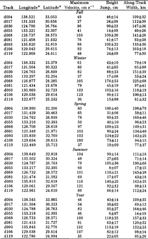
four seasons and for the first year of the T/P mission. The estimated maximum velocities, height jumps, and along-track width are listed in Table 3. These parame-

ters fluctuate over seasons, and, in general, high values

occur in the spring and summer and low values occur

in the fall and winter. Because we are only estimat-

ing two parameters instead of four in the least squares, the correlations between the estimated parameters are generally low (most below 20%). The high and low cor- relations are reflected as the large and small standard

deviations of the estimated parameters in Table 3. As

we examined the goodness of fit for all the tracks by

visual comparison, we found that the hyperbolic model

seems to work very well for the Kuroshio area. Figure

8 shows two typical comparisons, using tracks dl19 and

d017. Also, for all the tracks we found that the best

data extent for model fitting is within 100 km to the axis.

Figure 9 shows the filtered along-track SST values

and the locations where Vma• were found. As stated

before, the locations of Vma• correspond to the axis of

the Kuroshiol

Figure

10 shows

the locations

of Vmax

and the filtered SST from the 1-year data. In Figure 10

we also make a comparison of the SST by using two dif-

ferent geoid models as the level surface: the altimetric- gravimetric geoid and the geoid from OSU91A to degree 360. The OSU91A geoid has a resolution of 50 km and certainly cannot fully account for the complex bottom topography along the path of the Kuroshio. Because of its relatively low resolution, with the OSU91A geoid,

one cannot tell whether the steep slope in the computed

SST is due to the gravity signal or oceanographic signals

such as the Kuroshio front, and this is why in Figure 10 (lower panel) we cannot identify the location of the Kuroshio with the OSU91A geoid. Furthermore, we treated the locations of the path as a function of the along-path distance, namely

- (22)

where s is the along-path distance. Then we fitted a spline to the observed locations to obtain the path of the Kuroshio. Note that Akima's spline [de Boor, 1978] was used to avoid large oscillations due to the unequally spaced knots. Figure 11 shows the com-

puted paths for the four seasons and for one year with

the altimetric-gravimetric geoid as the level surface. Also, the path from the 32-year averaged Geomagnetic Electro-Kinetograph (GEK) data is compared with the path from the 1-year T/P data in Figure 11. GEK mea-

sures the velocity of currents utilizing the change of ge-

omagnetic field caused by the flow of water; see Pickard and Emery [1982] for more details about the principle of GEK. The GEK path is obtained by digitizing Figure 2 of Qiu et al. [1990]. In general, the GEK path and the 1-year altimeter path agree very well. The GEK path follows the 200-m isobath after leaving Taiwan, whereas the altimeter path shifts about 0-50 km to the west of this isobath. The highly focused paths in all seasons at about 32øN, 132øE are in good agreement with the observations by Mizuno and White [1983]. Due to the large cross-track spacing of the T/P, the resolution of the altimeter path is limited; for example, the altimeter path cannot account for the sharp turn of the Kuroshio

at about 30 oN, 129 øE.

To quantify the seasonal variability of the Kuroshio,

we again use the estimated parameters in Table 3. For

each of the tracks we calculate the standard deviations of the parameters based on the four values in the four

seasons. The standard deviations may be treated as the

variabilities. It is found that the mean variabilities in

path, maximum velocity, height jump, and width are

22 km, 15 cm s -•, 19 cm, and 27 km, respectively.

The 19-cm height jump corresponds to 9.5-Sv baroclinic

transport. If one accepts the idea that the percentage

variability is the ratio between the standard deviation

and the mean value, it is found that the average per- centage variabilities in maximum velocity, height jump, and width are 19%, 28%, and 24%, respectively. Fig- ure 12 shows the along-path variabilities for the axis, maximum velocity, height jump, and width. One sees from Figure 12 that all the variabilities are relatively large near the northeast coast of Taiwan and the begin- ning point of the Kuroshio Extension (at about 33øN, 137øE). A spot near 28øN, 128øE where the Kuroshio is about to make a sharp turn to the east also shows large variabilities in height jump, and width. Over the south coast of Japan the path variability is small, but the variabilities in maximum velocity, height jump, and width are large. Numerous studies have been devoted to the seasonal variability of the Kuroshio northeast of Taiwan [e.g., Chern et al., 1990; Chuang and Wu, 1991; Hu and Chang, 1992; Tang and Yang, 1993]. Some au- thors [e.g., Hu and Chang, 1992] attribute the variabil-

ity to local phenomena such as monsoon, whereas some

[e.g., Tang and Yang, 1993] believe that the variabil- ity is triggered by a remote phenomenon such as the change in the behavior of the North Equatorial Current. Abundant studies on the time-varying Kuroshio south

6324 HWANG: KUROSHIO'S VARIABILITY USING GEOID AND TOPEX/POSEIDON

Table 3. Estimated Parameters Associated With the Kuroshio Current in Four Seasons and One Year

Maximum Height Along-Track

Track Longitude a Latitude a Velocity, cm s -• Jump, cm Width, km Fall d004 138.521 33.053 49 464-14 1094-32 d017 131.333 30.656 27 244-08 1124-39 d030 124.790 26.764 86 904-22 1474-36 d055 133.221 32.397 41 144-09 404-26 d068 126.737 28.573 103 1094-20 1414-26 d081 121.458 21.632 76 414-17 934-38 d093 135.820 32.819 88 1004-22 1334-30 d106 129.042 29.615 92 744-13 1034-18 d119 122.968 24.611 48 244-09 774-30 Winter d004 138.332 33.379 61 424-10 794-18 d017 131.504 30.322 80 414-05 654-08 d030 124.765 26.809 82 884-23 1514-39 d055 133.297 32.254 37 174-08 534-24 d068 126.877 28.285 105 1764-53 2254-68 d081 121.434 21.678 79 454-19 974-41 d093 135.869 32.723 102 1024-16 1184-19 d106 129.038 29.614 123 964-12 1004-13 d119 122.677 25.232 36 154-08 614-32 Spring d004 138.990 32.206 60 1004-40 1984-79 d017 131.429 30.463 65 314-06 594-11 d030 124.762 26.810 78 894-25 1604-46 d055 133.216 32.393 50 404-10 964-23 d068 126.706 28.618 97 1094-23 1494-31 d081 121.348 21.871 103 804-24 1344-40 d093 135.839 32.769 102 1244-22 1424-25 d106 129.034 29.613 100 734-11 944-15 d119 122.449 25.712 37 194-09 774-37 Summer dO04 138.649 32.818 104 994-14 1114-16 d017 131.502 30.324 48 274-05 714-14 dO30 124.787 26.763 78 1054-36 1904-66 d055 133.217 32.395 60 84-07 174-15 d068 126.732 28.572 101 1104-21 1454-28 d081 121.474 21.582 69 174-07 434-18 d093 135.815 32.818 116 1404-25 1424-25 d106 129.061 29.567 121 924-12 984-13 d119 122.961 24.610 89 664-14 1124-24 Year d004 138.545 33.005 46 434-14 1094-35 d017 131.504 30.323 54 304-05 694-12 d030 124.788 26.763 82 954-27 1644-46 d055 133.218 32.395 46 64-07 144-19 d068 126.733 28.571 100 1184-25 1574-33 d081 121.413 21.727 91 634-17 1204-32 d093 135.843 32.770 101 1134-19 1324-23 d106 129.038 29.614 107 824-12 984-14 d119 122.786 24.994 35 224-05 954-20

aLongitude and latitude specify the location of maximum velocity.

of Japan are also available [e.g., Taft, 1972; Mizuno and White, 1983]. In particular, Mizuno and White [1983] attribute most of the variability south of Japan to a standing wave and a propagating wave in the Kuroshio

System.

Large Scale Circulation Over the

Western Pacific and Its Impact on the

The Kuroshio Current is initiated by the North Equa- torial Current [Hu and Chang, 1992] which is the equa-

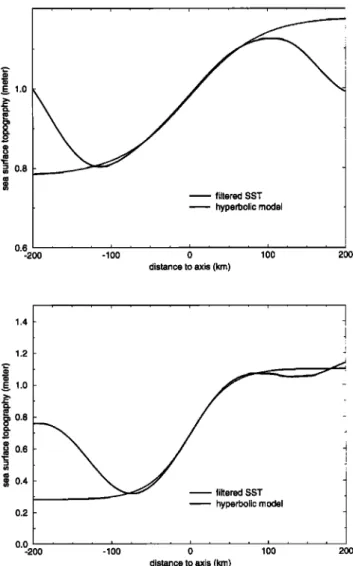
HWANG: KUROSHIO'S VARIABILITY USING GEOID AND TOPEX/POSEIDON 6325 • o.s filtered SST hyperbolic model 0'•200 -100 0 100 200 distance to axis (km) • 1.0 • • 0.8 o 0.6 ß 0.4 filtered SST hyperbolic model 0.2 0'0-200 -100 0 100 200 distance to axis (km)

Figure 8. Comparisons between the filtered SST and the hyperbolic models for (top) track d119 and (bot-

tom) track d017. The SST values

are from the 1-year

data. The zero distance corresponds to the point of maximum velocity, and the distance is negative before

this point.

torward arm of the subtropical gyre that spans the en- tire Pacific Ocean lapel, 1987]. The subtropical gyre

is clearly visible in a low degree spherical harmonic ex-

pansion

of the T/P SST; see,

e.g., Tapley

et al. (1994b)

other than the spherical harmonic expansion is needed

to identify the gyre. We use the median filter [Naess and Bruland, 1989] to do this. The median filter per- forms the best comparing to other filters such as the Gaussian filter, the boxcar filter (simple average), and the cosine filter. By "best" we mean the resulting SST agrees best with historical data in the overall structure of Pacific's circulation system. The next question is

how to determine the filter width. A filter width corre-

sponds to the maximum degree in a spherical harmonic

expansion. Thus, e.g., filter widths of 2001, 1334, 1000,

834, and 556 km correspond to maximum degrees of 10,

15, 20, 24, and 36, respectively. Figure 13 shows the

SST and the patterns of the geostrophic flows over the

Western Pacific in four seasons using a filter width of

1334 km. Figure 13 depicts circulation systems similar

to the results by other researchers working on the T/P

SST, e.g., Tapley et al. [1994b], Nerem et al. [1994], and Knudsen [1994]. The most pronounced difference in the four SST maps is the structure of the str½?m]ines east and north of Taiwan. Also, a distinct high over the Philippine Sea is found in summer, fall, and winter. This high is also found by Tapley et al. [1994b, Plate 5] and may be closely related to the annual cycle detected by Knudsen [1994, Plate 1]. The high is believed to be caused by the annual heating [Tapley et al., 1994b].

Now turning to the South China Sea, one sees from Figure 13 very distinct structures of SST in the four seasons. In the summer the sea surface rises by about 10 cm with respect to the sea level of winter. In the spring a warm ring with a radius of about 300-400 km and the center at about 15øN, 113øE is clearly visible and in the summer it becomes somewhat degenerated, but in the fall and winter it shows no sign of existence. At

this 1334-km spatial scale the flows in the South China

Sea are consistently clockwise. The rise of the sea level in spring and summer is probably due to heating, but not the spill of the water from the Pacific, because in

these two seasons the flow vectors at Bashi Channel are

pointing toward the Pacific Ocean. On the other hand,

in the fall and winter the Kuroshio enters the South China Sea at about 20 oN via the Bashi Channel when

the gyre's energy is the lowest.

Previously, we mentioned the possible causes of the Kuroshio's variability northeast of Taiwan. We will now see the link between the variability and the kinetic en- ergy of the subtropical gyre at the Western Pacific. The mean kinetic engergy per unit mass at a geographical location (•b, •)is defined as [Garraffo et al., 1992]

-

where v is the geostrophic velocity. Assuming a con-

stant thickness for the layer of the geostrophic flow and

a constant water density, the spatially averaged mean kinetic energy per unit mass over the studied area is

i i /A

v2(c)'A)

dA

(24)

where A is the area. The square root of Kr• is propor-

tional to the rms velocity of the geostrophic flow'

(2s)

rms velocity

- •

(•b,

A)

dA

which may be used as a descriptor for the dynamics of

the geostrophic flow. Using a filter length of 1334 km for

the SST and a numerical integration over the Western Pacific, we obtained with (25) rms velocities of 34.8, 38.4, 34.4, and 34.8 cm s -• for the spring, summer, winter, and fall, respectively. Since the width of the

Kuroshio front is of the order of 100 km, the calculated

6326 HWANG: KUROSHIO'S VARIABILITY USING GEOID AND TOPEX/POSEIDON

120 ø 125 ø 130 ø 135 ø 140 ø

35 ø -v •:•.

spring

,,:,oo:.:•._•?...-"

_','.,

_c•,..',...

_{•.• ,"0 ,}

'•••i•..r

'•

',,.¾.' • '•9':_tJ_,::7,, • ,-::•...- ::•..,,:!

'•.

•..,'•"

-.":

....

.."':.:'-":•:..

:.

•:•.½.•'•',-•':•...'"•,

:"-'.,

•. .•::,

%•,, I

,,:':..::-'

,..•i • -•..:• 4•::<...•

:.:.•.:.'..'

,•

:. .•:,•...

oo.=._.

:•:ii'?

•.

..½,.•.

:". "•.-'•J•. •.{

." .',ii•?."'.-.'-'.:-".,''•,.'..-,"--'...i:..-...,'"-:

'•:':}•,,

:'•_..•

I

... : •""'"'?':"-'

' ...

:•?:.'•.• '."• ,'?".

• 'i•.,.,

,-'

•.•..

. . - .••..

.•.-...

- :.,

...--.

..•

•:?...•.

. '•!:;.

: : : ....

:-:

.._

,

}(::::.-."-'_:_

•..•

...

,

...

•.• . •.-...-•...•...

. _

. . .••••

...:..;

""'"•i '"

i•"'{'}':

•'":'

'::'

... "'r

l*igure 9. The filtered along-track SST in four seasons. The Gaussian filter with a width of

$0 km is used. The crosses

mark the locations

of the maximum

velocities,

corresponding

•o the

axes of •he Kuroshio. The 100-cm bar shows the scale of SST measured perpendicular from the

ground track.

tered SST are independent of [he front of the Kuroshio along each of the T/P ground tracks. Figure 14 com- pares the gyre's rms velocities and the Kuroshio's max- imum velocities, height jumps, along-track width, and

distances of the axis to the mean axis northeast of Tai-

wan, which are taken from Table 3 at track dll•. Figure 14 shows that although [he data used are very sparse,

the gyre's rms velocities may be correlated with the first three parameters. This means that the Kuroshio's variability northeast of Taiwan may be triggered by the change of the gyre's kinetic engergy. When the gyre gains its maximum kinetic energy in the summer by perhaps heating, the Kuroshio's velocity, height jump

(equivalently

the baroclinic

transport),

and width be-