以高階緊致差分格式的方法模擬曲線受到曲率觸發的相關運動

全文

(1)Department Engineering Science and Ocean Engineering College of Engineering. National Taiwan University Bachelor Degree Thesis. On a high-order combined compact finite difference scheme for simulating the evolution of a mean curvature driven interface. Haw-Liang Wen. Professor Wen-Hann Sheu. 107 5 May 2018.

(2)

(3) Contents Content. 1. List of Figures. 2. List of Tables. 3. 1 XÅ. 4. 2 Abstract. 5. 3 Introduction. 6. 4 Level set equation. 8. 5 Numerical method. 11. 5.1 5.2. Optimal third-order TVD Runge-Kutta temporal scheme . . . . . . . . Combined compact finite di↵erence scheme for spatial derivative terms. 12 13. 5.3. Distance reinitialization . . . . . . . . . . . . . . . . . . . . . . . . . .. 14. 6 Numerical results 6.1 Order of reinitialization . . . . . . . . . . . . . . . . . . . . . . . . . . .. 18 18. 6.2 6.3 6.4. Validation . . . . . . . . . . . . . . . . . . . . . . . . . . . . . . . . . . Prediction of motion of curves driven by mean curvature flow . . . . . . Comparison of solutions obtained by CCD and second-order centered schemes . . . . . . . . . . . . . . . . . . . . . . . . . . . . . . . . . . . 6.4.1 Task 1, (!1 , !2 ) = (0, 0) . . . . . . . . . . . . . . . . . . . . . .. 25. 6.4.2. 25. 6.4.3. Task 2, (!1 , !2 ) = (5, 6) . . . . . . . . . . . . . . . . . . . . . . Task 3, (!1 , !2 ) = (5, 12) . . . . . . . . . . . . . . . . . . . . .. 19 19 24. 26. 7 Concluding remarks. 26. References. 27. 1.

(4) List of Figures 1. 2. 3. Validation 1, present (a)-(d), ref.[18], (e) Star-shaped curve’s motion by mean curvature. The computation is carried out in 300 ⇥ 300 grids, with the mesh size of h = dx = dy and the time step of dt = 0.0001 ⇥ h . . .. 7. curvature. The computation is carried out in 300 ⇥ 300 grids, with the mesh size of h = dx = dy and the time step of dt = 0.00001 ⇥ h. . . . .. 9. Validation 2, present (a)-(d), ref.[18], (e) Wound spiral motion by mean. Case 1. Computation is carried out in 200x200 grids in a 10 by 10 domain, with the mesh size of h = x = y = 0.05 and the time step of. 4. t = 0.01 ⇥ h. Red line denotes the solution obtained with. reinitialization procedure while green dashed line denotes the solution obtained without reinitializtion procedure. . . . . . . . . . . . . . . . . Case 2. Computation is carried out in 200x200 grids in a 10 by 10. 10. domain, with the mesh size of h = x = y = 0.05 and the time step of t = 0.01 ⇥ h. Red line denotes the solution obtained with. 5. reinitialization procedure while green dashed line denotes the solution obtained without reinitialization procedure. . . . . . . . . . . . . . . . Case 3. Computation is carried out in 200x200 grids in a 10 by 10. 15. domain, with the mesh size of h = x = y = 0.05 and the time step of t = 0.01 ⇥ h. Red line denotes the solution obtained with reinitialization procedure while green dashed line denotes the solution 6. 7 8. 9 10. obtained without reinitialization procedure. . . . . . . . . . . . . . . . Plots for indicating the relation among , N ( ) and r2 along the curve (s) at t = 1.0 for case 1. (a) with reinitialization procedure; (b) without reinitialization procedure . . . . . . . . . . . . . . . . . . . . . . . . . . Plots for !N along the curve (s) at t = 1.0 for case 1. (a) with reini-. 16. tialization procedure; (b) without reinitialization procedure . . . . . . . Plots for indicating the relation among the , N ( ) and r2 along the curve (s) at t = 2.0 for case 1. (a) with reinitialization procedure; (b) without reinitialization procedure . . . . . . . . . . . . . . . . . . . . . Plots for !N along the curve (s) at t = 2.0 for case 1. (a) with reinitialization procedure; (b) without reinitialization procedure . . . . . . . Plots for !N along the curve (s) at t = 0.05 for case 3. (a) with. 20. reinitialization procedure; (b) without reinitialization procedure . . . .. 22. 2. 19. 21 21.

(5) 11. Task 1. Comparison of the solutions sought at di↵erent times by applying the CCD scheme and the second-order centered di↵erence scheme. The computations are carried out with h = dy = dx = 0.05 and dt = 0.01⇥h.. 12. (a) t = 1.0; (b) t = 2.0 . . . . . . . . . . . . . . . . . . . . . . . . . . . Task 2. Comparison of the solutions sought at di↵erent times by applying. 24. the CCD scheme and the second-order centered di↵erence scheme. The computations are carried out with h = dy = dx = 0.05 and dt = 0.01⇥h. 13. (a) t = 0.0625; (b) t = 0.250 . . . . . . . . . . . . . . . . . . . . . . . . Task 3. Comparison of the solutions sought at di↵erent times by applying. 25. the CCD scheme and the second-order centered di↵erence scheme. The computations are carried out with h = dy = dx = 0.05 and dt = 0.01⇥h. (a) t = 0.0625; (b) t = 0.250 . . . . . . . . . . . . . . . . . . . . . . . .. 26. List of Tables 1 2. Computation flow chart of reinitialization procedure. . . . . . . . . . . Order of several numerical schemes in the problem introduced in [20] and. 18. [19]. . . . . . . . . . . . . . . . . . . . . . . . . . . . . . . . . . . . . .. 18. 3.

(6) 1. XÅ. ,vÑÓ⇡/Âÿæ∫ÑD. ˚Ó⌃<✏(CCD). -M4s∆. π’(level set. method)!ÏÚ⁄ÑK’⇥(K’π↵✏- Ú⁄ÑK’/◊0Úá(Ú⁄⌦ÑÓ p ¯| ⌘⌘⇤⌃%‘⇤( ˚Ó⌃<✏Â -.Ó⌃ óÚá &9⁄ ˚⌫ÑóãÑ‘⇤ ˇ⇥ BìÑ‚c Ñqˇ. o:(i. ,v/°(. x<π’‚czìÆ⌃⇧ ºÚ⁄K’Ñq éTVD Runge-Kuttaπ’⇥Õ›‚ ºTH. _⇤(,v-ì1óãÜ2L. ÷⇥. ,vÑpL!^/¢ Ú⁄⌦⌅fiÑÚá⇤ÇU®Bìä Ú⁄Ñä (π↵ ✏-/1 ⁄'⌥^⁄'⇧ i⇧@/M⇥,v⇤s0 ÷⁄'⌥^⁄'(K’ -Ñqˇ↵¶⇥. Keywords:. PÓ⌃’. 4s∆. ’. D 4. ˚Ó⌃<✏. Úá. …n…ØóP.

(7) 2. Abstract. This study is aimed to develop a high-order finite di↵erence scheme to simulate the mean curvature equation for accurately predicting the time-evolving mean curvature driven interface. Within the semi-discretization framework, the optimal third-order accurate temporal scheme is applied for the approximation of the time derivative term. In a threepoint grid stencil, a combined compact di↵erence scheme has been developed for o↵ering a fifth-order spatial accuracy for the first-order and second-order derivative terms shown in the level set equation for simulating mean curvature flow. In the simulation of the mean curvature equation, reinitialization procedure has been performed to improve the prediction of curve motion. The aim of this study is to give insights into the issue about ”how a mean curvature driven curve is varied with time”. Two mechanisms leading to the change of curve slope are attributed partly to the damping Laplacian operator and partly to the embedded nonlinear di↵erential operator. These mechanisms have been studied in detail with respect to the curvature of curve. The e↵ect of performing reinitialization is also studied numerically.. Keywords: finite di↵erence method, level set method, combined compact di↵erence scheme, mean curvature, Laplace operator 5.

(8) 3. Introduction. Study of geometric evolution of curves or surfaces has been an important subject in mathematical society. Research into this type of physical and mathematical problems has led to several systems of nonlinear partial di↵erential equations. Many physical processes about the propagation of material interface, free surface or interface flow development, and the growth of crystal can be simulated by solving the corresponding partial di↵erential equations governing the evolution of geometrical curves or surfaces. An accurate capturing of these time-evolving curves and surfaces is essential for gaining a better understanding of the convection and di↵usion phenomena in many curve and surface processing applications. In computer graphics, the processing of triangulated surfaces, for example, is a fundamental topic worth of investigation as well [1]. In the mathematical modeling of a geometric evolution of curve or interface , one can represent it implicitly as the zero level set of a continuous function . This corresponds to writing = {x| (x, t) = 0} for a surface. In many problems ranging from a two-fluid flow to a crystal growth process, the evolution is subject to the normal speed of . The time evolution of the level set function for this class of problems can be expressed in a general form as @@t + uN |r | = 0, where the normal speed of di↵ers from each other depending on their involved physical mechanisms leading to the change of . For the mean curvature flow problem, uN = , where  (⌘ r · ~n) is the mean curvature of , r· is the surface divergence di↵erential operator, and ~n denotes the outward normal vector of the curve of interest. The level set equation for modeling the motion driven by mean curvature becomes @ @t. r·(. r )|r | = 0 |r |. (1). Surface di↵usion occurring in film growth is the other example of the physical e↵ect that is relevant to the evolution of geometric curves. For this case, surface moves with the normal velocity rs · (rs ) under surface di↵usion, where rs = r n ˆ (ˆ n · r). The change of the level set function. for surface di↵usion corresponds to. @ + rs · rs |r | = 0 @t. (2). Due to the similarity presenting in two important classes of equation, it is worthwhile for r us to investigate the equation generalized as @@t + uN |r | = 0, where uN = r · ( |r ) |. for mean curvature flow while uN = rs · (rs ) for surface di↵usion flow. In our study employing the level set method, the focus will be on the evolution of geometric curve driven by its mean curvature. Motions of curves subject to surface di↵usion have been 6.

(9) 0.2. 0.1. 0.1. 0. 0. y. y. 0.2. -0.1. -0.1. -0.2 -0.2. -0.1. 0. 0.1. -0.2 -0.2. 0.2. -0.1. 0. x. 0.0004. (b) t = 0.0004. 0.2. 0.2. 0.1. 0.1. 0. 0. y. y. (a) t = 0. 0.1. 0.2. x. -0.1. 0.0008. -0.1. -0.2 -0.2. -0.1. 0. 0.1. -0.2 -0.2. 0.2. x. (c) t = 0.0008. -0.1. 0. 0.1. 0.2. x. 0.0012. (d) t = 0.0012. 0.0016. (e). Figure 1: Validation 1, present (a)-(d), ref.[18], (e) Star-shaped curve’s motion by mean curvature. The computation is carried out in 300 ⇥ 300 grids, with the mesh size of h = dx = dy and the time step of dt = 0.0001 ⇥ h. 7.

(10) predicted by di↵erent research groups [7, 8, 9] using the level set method. The content of this paper will be organized as follows. In section 2, the level set equation for the modeling of a time-evolving curve driven by mean curvature and surface di↵usion will be presented. Some important features of this equation cast in level set function will be pointed out. The numerical method will be introduced in section 3. In section 4, the nonlinear parabolic equation will be solved using the high-order compact finite di↵erence scheme formulated in a three-point grid stencil. Discussion of the simulated results will be given in section 4 as well. Finally, we will draw some concluding remarks in section 5.. 4. Level set equation. In real life, di↵usion process, which is well-known as @c = Dr2 c, equilibrates spatial @t change of a physical concentration c. Such a process involving the molecular di↵usion coefficient D happens all the time and is irreversible. For the evolution of a smoothly distributed surface x, the Eulerian Laplacian di↵erential operator r2 is replaced with the Laplace Beltrami di↵erential rM , leading to the so-called geometric di↵usion analogue for the coordinate x on a surface S. @x = r2M (t)x (3) @t According to the theory of di↵erential geometry [2], the Laplace Beltrami operator defined on a surface S is identical to the mean-curvature vector h(x)n(x), implying that (4) r2M x = h(x) n(x) Geometric di↵usion is commonly referred to as mean curvature motion, thereby leading to the following di↵erential equation @x = h(x) n(x) (5) @t In the above, h(x) denotes the mean curvature and n(x) can be expressed in terms of the level set function as n(x) = |r | (6) The mean curvature, which is defined as the sum of the two principal curvatures, can r ), where the distance function is negative inside the curve. be written as r ·~n = r · ( |r | In two-dimensional domain, the curvature of a curve can be explicitly expressed as h(x) = r · (. 2 xx y. 2 x y+ ( 2x + 2y )3/2. r )= |r | 8. 2 yy x. (7).

(11) 0.04. 0.04. 0.02. 0.02. 0. 0. y. 0.06. y. 0.06. -0.02. -0.02. -0.04. -0.04. -0.06 -0.06. -0.04. -0.02. 0. 0.02. 0.04. -0.06 -0.06. 0.06. -0.04. -0.02. x. 0. 0.02. 0.04. 0.06. x. (a) t = 0. 0.0001. (b) t = 0.0001. 0.0002. 0.06 0.04 0.04 0.02 0.02. y. y. 0 0. -0.02 -0.02. -0.04. -0.04. -0.06 -0.06. -0.04. -0.02. 0. 0.02. 0.04. -0.06 -0.06. 0.06. x. (c) t = 0.0002. -0.04. -0.02. 0. 0.02. 0.04. 0.06. x. 0.0003. (d) t = 0.0003. 0.0004. (e). Figure 2: Validation 2, present (a)-(d), ref.[18], (e) Wound spiral motion by mean curvature. The computation is carried out in 300 ⇥ 300 grids, with the mesh size of h = dx = dy and the time step of dt = 0.00001 ⇥ h.. 9.

(12) 8. 8. 8. 6. 6. 6. y. 10. y. 10. y. 10. 4. 4. 4. 2. 2. 2. 0. 0. 2. 4. 6. 8. 0. 10. 0. 2. 4. 6. 8. 0. 10. 6. (a) t=0.0. (b) t=0.25. (c) t=0.5. 8. 6. 6. 6. 4. 4. 4. 2. 2. 2. 4. 6. 8. 0. 10. 8. 10. 8. 10. y. 8. y. 8. y. 10. 2. 4. x. 10. 0. 2. x. 10. 0. 0. x. 0. 2. 4. 6. 8. 10. 0. 0. 2. 4. 6. x. x. x. (d) t=1.0. (e) t=1.5. (f) t=2.0. Figure 3: Case 1. Computation is carried out in 200x200 grids in a 10 by 10 domain, with the mesh size of h = x = y = 0.05 and the time step of t = 0.01 ⇥ h. Red line denotes the solution obtained with reinitialization procedure while green dashed line denotes the solution obtained without reinitializtion procedure.. Given the definitions of n(x) and h(x), the partial di↵erential equation for geometric di↵usion can be derived in terms of a level set function as @ @t. |r | r · (. r )=0 |r |. (8). In this study, we aim to investigate the Cauchy problem that involves the HamiltonianJacobi equation (8) cast in the first order form. Equation (8) can be also expressed di↵erently as follows after a mathematical manipulation. @ = r2 @t where N( ) =. N( ). @|r | r = · r(|r |) @n |r |. (9). (10). Equation (9) elucidates that surface di↵usion has a role to play in the mean curvature flow equation. The level set method, developed by Osher and Sethian [4], will be applied to predict the motion of interface in a domain of two dimensions. Level set methods have been 10.

(13) applied with great success to predict a wide variety of problems. One can refer to the review papers [5, 6, 7]. For the level set function. in a flow field u, it is mathematically. modeled by the well-known pure advection equation. @ +u·r =0 (11) @t If the evolution of curves or surfaces involves only the normal component of u, we can get @ + un |r | = 0 (12) @t By comparing the equation (8) with the nonlinear parabolic equation (12), we are led to get the normal speed of the surface un =. r·(. r ) |r |. (13). As we mentioned in the introduction, it is worthy to point out the similarity and di↵erence between the mean curvature flow and the surface di↵usion flow. By virtue of the classification of these two equations, both of them are parabolic equations but they are driven by di↵erent normal speeds related to the curvature. Equation (13) shows that the normal speed of mean curvature flow is the mean curvature. As for equation (2), the normal speed of surface di↵usion flow is un = r2s  = r2 . (~n · r)(~n · r). (14). The physical meaning of the term on the right-hand-side of equation (14) is that the normal speed of curve in surface di↵usion flow depends only on the physical di↵usion of curvature along the curves. The first term on the right-hand-side denotes the di↵usion of curvature over the space, and the second term stands for the di↵usion on its normal direction of the curve. The result enlightens the presence of the tangential di↵usion of curvature along the curves. It is worthy to note here that the difficulty of solving equation (12) with respect to two di↵erent types of curve motion subjected to di↵erent normal speeds, as shown in eq. (13) and eq. (14), for an interface motion is that it is nonlinear and is quite sti↵. We are therefore motivated to propose a numerically very accurate and computationally more efficient method.. 5. Numerical method. The primary difficulty of numerically solving the level set equation for a motion driven by mean curvature is that the parabolic equation (12) is sti↵. Implicit method is therefore the method of choice for the finite di↵erence approximation of the HamiltonianJacobi equation for the modeling of curvature flow motion [3]. Moreover, equation (12) 11.

(14) is nonlinear. It is therefore a straightforward practice for us to implement implicit numerical method in this study to circumvent the computational difficulty. In this paper, we rewrite equation (12) in the form of t. = L( ). (15). where un |r |. L( ) =. (16). The solution to the parabolic equation (15) will be sought subject to the initial condition given by (x, t = 0) =. (17). 0. The semi-discretization scheme will be employed to solve the equation (15). The time discretization is performed first using the Runge-Kutta method with the initial condition (17) and, then, the spatial discretization will be performed. 5.1. Optimal third-order TVD Runge-Kutta temporal scheme. The Runge-Kutta method for equation (15) can be expressed in a general form as follows for i = 1, ..., m [10]. (i). =. i 1 X. (k). ↵ik. +. t. ik. L(. (k). ). (18). k=0 0. =. n. ,. m. =. n+1. (19). In the above class of Runge-Kutta schemes, the coefficients ↵ik and ik shall be properly chosen so that application of the resulting scheme can not only yield higher order accuracy but also can maintain numerical stability in whatever the norms are [11]. We are therefore motivated to adopt a high order TVD (total variation diminishing) time discretization scheme [11]. Application of this class of schemes implies that the total variation of the numerical solution is not allowed to increase in the sense that P T V ( n+1 ) < T V ( n ), where T V ( ) = i | i+1 i |. Equation (18) is TVD provided that ↵ik , ik > 0 under a suitable time step restriction. Our objective of employing the TVD Runge-Kutta scheme is to retain the TVD property while high order temporal accuracy can be maintained. To achieve the goal of obtaining high-order solution accuracy and enhancing numerical stability, it is required that both coefficients ↵ik and ik shown in equation (18) be non-negative. Therefore,. 12.

(15) the optimal third-order TVD Runge-Kutta method given in [11] is adopted. 1. =. 2. =. n+1. n. 3 4 1 = 3. t L( n ) 1 1 n t L( 1 ) + 1+ 4 4 2 2 n t L( 2 ) + 2+ 3 3 +. (20). The above scheme is stable subject to the CFL condition, by which we have c= 5.2. ↵ik t < min( ) i,k x ik. Combined compact finite di↵erence scheme for spatial derivative terms. Having discretized the temporal derivative term in equation (20), we proceed to the discretization of the spatial derivative terms L( n ), L( 1 ) and L( 2 ) shown in equation (20). The idea of applying the combined compact di↵erence (CCD) scheme proposed first by Chu and Fan [12] is to improve prediction accuracy when approximating the first and second order derivative terms without increasing the number of stencil points. The building block of our CCD scheme is to calculate the derivative of a function at an interior grid point together with the same derivative terms at the two adjacent points. With the ability of improving solution accuracy with lower computational cost, it is quite promising that CCD scheme can be implemented for large scale computation. In equation (7), one can see clearly that calculation of the curvature of a curve. involves. computing the values of x , y , xx , yy and xy . To get a spectral-like resolution for these derivatives in a grid involving only three stencil points, i 1, i, i + 1, the centered CCD scheme is adopted in a domain with uniform spacing h = x = y. This CCD scheme calculates the derivative terms x and xx shown in (7) implicitly from the following two equations for P ⌘ x and Q ⌘ xx . h 7 (Pi+1 + Pi 1 ) + Pi (Qi+1 Qi 1 ) = 16 16 1 9 (Pi+1 Pi 1 ) (Qi+1 + Qi 1 ) + Qi = 8h 8. 15 ( i+1 16h 3 ( i+1 2 h2. i 1). (21) i. +. i 1). All the coefficients shown in (21) have been derived underlying the modified equation analysis. Taylor series expansion has been performed on Pi+1 and Qi+1 with respect to Pi and Qi , respectively, to get the corresponding modified equations. The leading error terms in the modified equations are then eliminated to close the derivation of the two equations in (21). Similar idea can be employed to implicitly calculate the nodal values of y and yy by solving the resulting block tri-diagonal matrix. As for the value of 13.

(16) xy ,. of 5.3. it can be also computed by taking this mixed derivative term as the di↵erentiation y. with respect to x. Distance reinitialization. In the prediction of geometric evolution of a curve , one should prevent the level set function. becoming too flat or too steep near. that separates two fluids [4]. Avoidance. of this issue that has been known to arise more or less from the introduced discretization error necessitates the application of a distance reinitialization procedure. The level set function. governed by equation (8) should be replaced with the other signed distance function d(x, t), which denotes the signed distance of x to the closest point on . By definition, the signed distance function is di↵erentiable almost everywhere, and its gradient should satisfy the eikonal function |r | = 1 in the domain of interest. According to [13], the value of (x, t) governed by (12) is reinitialized to the steady solution of the following equation for (x, t), subject to (x, ⌧ = 0) = (x, t) = 0 , @ + sgn( @⌧. 0). (|r |. 1) = 0. (22). In the above, ⌧ denotes the artificial time and sgn( ) = 2H( ) 1, where H( ) is known as the Heaviside function. Solution to equation (22) is sought with the time step of ⌧ = 0.25 x. In other words, as ⌧ ! 1 , the solution to equation (22) satisfies the eikonal function |r | = 1, and the reinitialization procedure is completed. The Heaviside function is the characteristic function, which 8 > 0, > > ◆ if < ✓ 1 H( ) = , if | 1 + ✏ + ⇡1 sin ⇡✏ 2 > > > : 1, if. is defined as <✏ |✏ >✏. It is noted that✏ is a small positive number with the value of ✏ = 1.5 x in this study. Such a chosen magnitude can give us a better convergent result [16]. Equation (22) governing the evolution of distance function (x, t) involves using the Heaviside function. in the physical domain ⌦. To avoid oscillatory solutions generated in the vicinity of , we apply the WENO (Weighted Essential Non-Oscillatory) spatial discretization scheme [14, 15] to get a high-resolution solution. In our employed closest point formulation of the distance function, the sign function sgn( ) is approximated by introducing a small positive parameter ✏ to replace equation (22) with the following smoothed redistancing embedding partial di↵erential equation. @ + 2H( @⌧. 0). 1 (|r | 14. 1) = 0. (23).

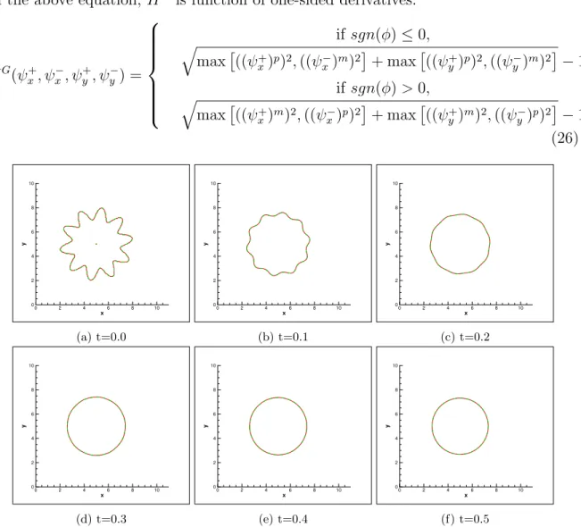
(17) In the above, the sign function has been replaced with a smoother version. Equation (23) can be also written into the following Hamiltonian-Jacobi form: ⌧. + sgn(. 0 )H(. ,r ) = 0. (24). where H( , r ) is the corresponding Hamiltonian. By employing Godunov spatial discretization, equation (24) can be further rewritten in terms of the one-sided derivatives + x,. ,. x. + y ,. y. as ⌧. + sgn( 0 )H G (. + x,. x. ,. + y ,. y. )=0. (25). In the above equation, H G is function of one-sided derivatives. 8 > if sgn( )  0, > > q > ⇤ ⇥ ⇥ > + )p )2 , (( m )2 + max (( < max (( ) x x H G ( x+ , x , y+ , y ) = > if sgn( ) > 0, > > q > ⇤ ⇥ ⇥ > : max (( x+ )m )2 , (( x )p )2 + max ((. 8. 8. 8. 6. 6. 6. 4. 4. 4. 2. 2. 2. 0. 0. 2. 4. 6. 8. 0. 10. 0. 2. 4. 6. 8. 0. 10. 4. 6. x. (a) t=0.0. (b) t=0.1. (c) t=0.2. 8. 6. 6. 6. 4. 4. 4. 2. 2. 2. 4. 6. 8. 10. 1. ⇤. 1 (26). 8. 10. 8. 10. y. 8. y. 8. y. 10. 2. 2. x. 10. 0. 0. x. 10. 0. + m 2 p 2 y ) ) , (( y ) ). ⇤. y. 10. y. 10. y. 10. + p 2 m 2 y ) ) , (( y ) ). 0. 0. 2. 4. 6. 8. 10. 0. 0. 2. 4. 6. x. x. x. (d) t=0.3. (e) t=0.4. (f) t=0.5. Figure 4: Case 2. Computation is carried out in 200x200 grids in a 10 by 10 domain, with the mesh size of h = x = y = 0.05 and the time step of t = 0.01 ⇥ h. Red line denotes the solution obtained with reinitialization procedure while green dashed line denotes the solution obtained without reinitialization procedure.. 15.

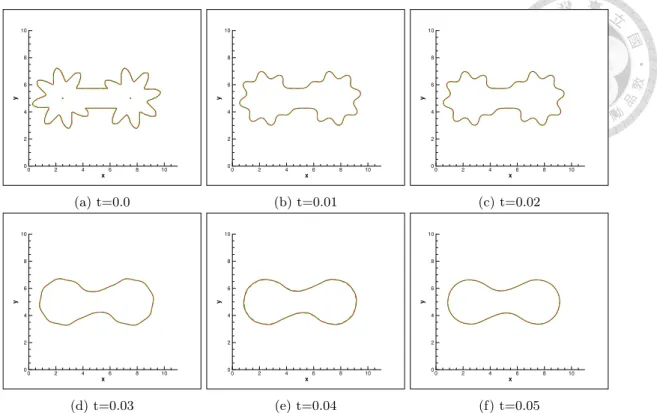
(18) 8. 8. 8. 6. 6. 6. y. 10. y. 10. y. 10. 4. 4. 4. 2. 2. 2. 0. 0. 2. 4. 6. 8. 0. 10. 0. 2. 4. 6. 8. 0. 10. 6. (a) t=0.0. (b) t=0.01. (c) t=0.02. 8. 6. 6. 6. 4. 4. 4. 2. 2. 2. 4. 6. 8. 0. 10. 8. 10. 8. 10. y. 8. y. 8. y. 10. 2. 4. x. 10. 0. 2. x. 10. 0. 0. x. 0. 2. 4. 6. 8. 0. 10. 0. 2. 4. 6. x. x. x. (d) t=0.03. (e) t=0.04. (f) t=0.05. Figure 5: Case 3. Computation is carried out in 200x200 grids in a 10 by 10 domain, with the mesh size of h = x = y = 0.05 and the time step of t = 0.01 ⇥ h. Red line denotes the solution obtained with reinitialization procedure while green dashed line denotes the solution obtained without reinitialization procedure.. Noted that the notations (#)p = max(#, 0) and (#)m = min(#, 0). The one-sided derivatives x+ , x , y+ , y are calculated as follows following the framework of WENO scheme. Consider a one-dimensional example, the definitions of x+ , x are respectively as follows + x. x. =. i. =. i. ˆ+. ˆ+. xi+1/2 ˆ. xi ˆ. xi+1/2. xi. i+1/2. i+1/2. i 1/2 1/2. (27). i 1/2 1/2. + The numerical fluxes of î+1/2 , î+1/2 are the Lipschitz continuous functions of sev+ , î+1/2 should be respectively eral neighboring values i . The numerical flux î+1/2 computed within the WENO framework of the right and left biased interpolations. Construction of the right-biased and left-biased numerical fluxes is given as follows [15, 17]. ˆ. i+ 12. ˆ+. i+ 12. = !1L î+ 1 ,L + !2L î+ 1 ,L + !3L î+ 1 ,L (1). (2). 2. =. !1R. ˆ(1)1 i+ 2. (3). 2. + ,R. !2R 16. ˆ(2)1 i+ 2. 2. + ,R. !3R. ˆ(3)1. i+ 2 ,R. (28).

(19) (k) (k) In the above, î+ 1 ,R and î+ 1 ,L (k = 1, 2, 3) are respectively expressed as 2. ˆ(1)1. =. ˆ(2)1. =. i+ 2 ,L. i+ 2 ,L. ˆ(3)1. i+ 2 ,L. 2. 1 3. 1 6 1 = 3. 7 6. 11 11 7 1 ˆ(1) i , i+ 1 ,R = i+1 i+2 + i+3 2 6 6 6 3 5 1 1 5 1 ˆ(2) i 1+ i+ i+1 , i+ 1 ,R = i+ i+1 i+2 2 6 3 3 6 6 5 1 1 5 1 ˆ(3) i+ i+1 i+2 , i+ 1 ,R = i 1+ i+ i+1 2 6 6 6 6 3. i 2. i 1. +. (29). The weighting coefficients wkR,L (k = 1, 2, 3) shown in (28) are nonlinear. This WENO scheme can make the linear di↵erential equation (23) to become its nonlinear counterpart. As a result, non-oscillatory solution can be possibly obtained. The coefficients wkR,L derived in [17] can yield the fifth-order accurate spatial discretization provided that ↵R,L ck !kR,L = P k R,L , ↵kR,L = R,L (30) ( k + "ˆ)2 k ↵k In the above,. R,L are k 12. itive number (10 k. the smoothness indicators of the k-th stencil, and "ˆ is a small pos-. ) introduced to prevent division by zero. The smoothness indicators. (k = 1, 2, 3) for the left-biased are shown as follows L 1 L 2 L 3. 13 ( 12 13 = ( 12 13 = ( 12 =. i 2. i 1. i. 1 + ( i 2 4 i 1 + 3 i )2 4 1 2 2 i + i+1 )2 + ( i 1 i+1 ) 4 1 2 i+1 + i+2 )2 + (3 i 4 i+1 + i+2 )2 4 2. i 1. +. i). 2. As for the smoothness indicators for the right-biased. k. (31). (k = 1, 2, 3), they are expressed. as R 1 R 2 R 3. 13 ( 12 13 = ( 12 13 = ( 12 =. i+1. i. i 1. 1 + (3 i+1 4 i+2 + i+3 )2 4 1 2 2 2 i+1 + i+2 ) + ( i i+2 ) 4 1 2 i + i+1 )2 + ( i 1 4 i + 3 i+1 )2 4 2. i+2. +. i+3 ). 2. (32). The optimal weights shown in (30) are c1 = 1/10, c2 = 6/10, c3 = 3/10, which yield the fifth order accuracy in the approximation of the spatial derivative terms. For clarification, the algorithm of the reinitialization procedure is summarized below:. 17.

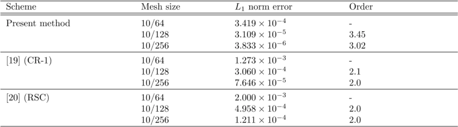
(20) • Beginning of the reinitialization procedure. – Iteration starts – • • • • • •. Calculate the smoothness indicators kR,L (k = 1, 2, 3) from equations (31) and (32). Compute the corresponding nonlinear weighting coefficients !kR,L (k = 1, 2, 3) from equation (30). + Calculate î+1/2 and î+1/2 with the nonlinear weighting coefficients from equations (28) and(29). Compute the one-sided derivatives from equation (27). Calculate H G from equation (26). Update by solving equation (??).. – Iteration stops until the solution reaches steady state condition – • As reinitialization procedure is completed, let. =. Table 1: Computation flow chart of reinitialization procedure.. 6 6.1. Numerical results Order of reinitialization. To show the order of method we used in reinitialization, we investigated the problem introduced in [20] and [19]. The level set function is initialized with the following equation in a computational domain ⌦ : [ 5, 5] ⇥ [ 5, 5]. p 3)2 + (y 3)2 3 x2 + y 2 0 = 0.1 + (x. To evaluate the order of our method, the L1 norm of the di↵erence e1 between the exact signed distance function and the numerical solution is determined by q 1 X numerical numerical 2 e1 = || exact ||1 = x2i,j + yi,j 3 i,j N⌦ ⌦ The corresponding L1 norm errors e1 obtained under di↵erent mesh sizes using di↵erent methods are listed in following table Scheme Present method. [19] (CR-1). [20] (RSC). Mesh size. L1 norm error 3.419 ⇥ 10 3.109 ⇥ 10 3.833 ⇥ 10. 10/64 10/128 10/256. 1.273 ⇥ 10 3.060 ⇥ 10 7.646 ⇥ 10. 10/64 10/128 10/256. 2.000 ⇥ 10 4.958 ⇥ 10 1.211 ⇥ 10. 10/64 10/128 10/256. 4 5 6 3 4 5 3 4 4. Order 3.45 3.02 2.1 2.0 2.0 2.0. Table 2: Order of several numerical schemes in the problem introduced in [20] and [19]. 18.

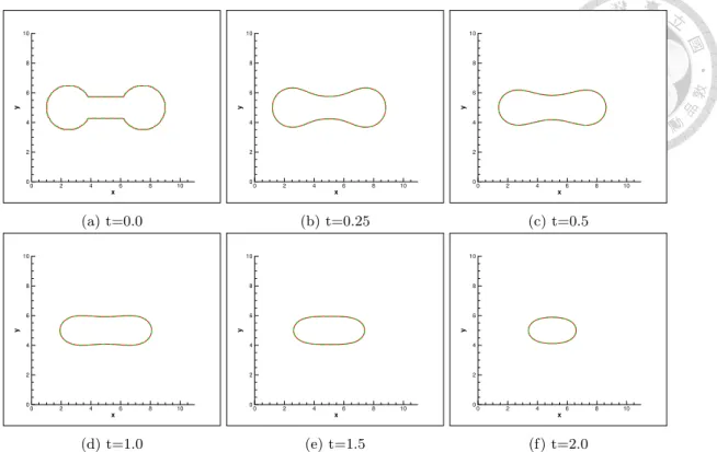
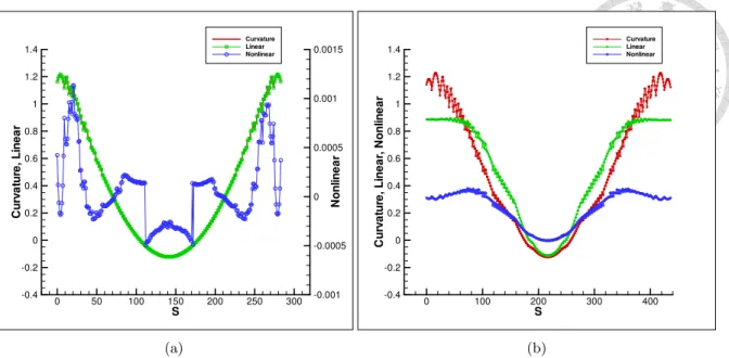
(21) Curvature Linear Nonlinear. 1.4. 0.0015. 1.2 0.001. 0.8 0.0005 0.6 0.4 0. Nonlinear. Curvature, Linear. 1. 0.2 0. -0.0005. -0.2. Curvature, Linear, Nonlinear. 1.2. -0.4. Curvature Linear Nonlinear. 1.4. 1 0.8 0.6 0.4 0.2 0. -0.2. 0. 50. 100. 150. 200. 250. 300. -0.001. -0.4. 0. 100. 200. S. S. (a). (b). 300. 400. Figure 6: Plots for indicating the relation among , N ( ) and r2 along the curve (s) at t = 1.0 for case 1. (a) with reinitialization procedure; (b) without reinitialization procedure. 6.2. Validation. Our validation studies were carried out by comparing the simulated results with the numerical result obtained by Osher and Sethian in [18]. Good agreement between two sets of the results can be clearly seen in figure 1 and figure 2 for the star-shaped and wounded spiral motions. The curves have the identical evolution subject to two initial conditions. Application of our proposed CCD scheme to predict mean curvature driven motion of curves is therefore justified. 6.3. Prediction of motion of curves driven by mean curvature flow. The linear part of the R.H.S. of equation (9) exhibits that the solution shall be smeared from a higher value to a lower value all over the space until the Laplacian of approaches zero. The source terms in R.H.S. of equation (9) including Laplacian and nonlinear terms are always nonzero since is the distance function. As a result, the motion of curve is always activated until it is shrunk to a point. Three cases of different initial curves are investigated in this section, namely the dumbbell-like, star-like and dumbbell-star-like curves. They are denoted as the cases 1, 2 and 3, respectively. We will also show how the applied reinitialization procedure a↵ects the motion of curve. Figure 3 shows the predicted motion driven by mean curvature for case 1. It can be observed that each point on the curve begins to shrink in di↵erent speeds along the curve. Curves with a higher curvature have a higher speed. The shape of the curve 19.

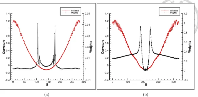
(22) Curvature Weights. 1.4. 0.05. Curvature Weights. 1.4. 1.2. 1.2. 1.2 1. 0.04 1. 1 0.8. 0.02 0.4 0.2. 0.01. 0.6. 0.6. 0.4. 0.4. Weights. 0.6. 0.8. Curvature. 0.03. Weights. Curvature. 0.8. 0.2 0.2. 0. 0 0. 0. -0.2 -0.4. -0.2. 0. 50. 100. 150. 200. 250. -0.01 300. -0.4. 0. 100. 200. S. S. (a). (b). 300. 400. -0.2. Figure 7: Plots for !N along the curve (s) at t = 1.0 for case 1. (a) with reinitialization procedure; (b) without reinitialization procedure. at t = 0.0 is gradually evolved to an ellipse at t = 2.0, and it can be expected that the curve will be finally evolved to a circle since it has the lowest surface energy in its physical meaning. From equation (9), it is revealed that the motion of the curve is attributed to the e↵ects of linear and nonlinear terms. It is worthy to know which source term is the dominant one in the time evolution and has a stronger e↵ect on the curve. Figures 6a and 6b show the relation among the curvature , linear source term r2 and nonlinear source term N ( ) for the solution at t = 1.0 with and without reinitialization. The relation is given along the curve (s) by introducing a parameter s. N ( ) is found to have a very small magnitude in comparison with that of r2 , implying that the evolution of the mean curvature driven curve is dominated by the di↵usion process. Another way to understand why equation (9) can be regarded as the linear di↵usion equation with reinitialization procedure is that r = 1 is satisfied when applying reinitialization procedure in every computational step. According to the definition of N ( ) in equation (10), it should be zero under a perfect reinitialization by which the derivative of a constant is zero. Since discretization error will be introduced more or less in the reinitialization step , the value of N ( ) shall not be exactly equal to zero. Reinitialization plays an important role in the motion of curve as it is shown in figure 6b, since this procedure redistributes r2 and N ( ) but without a↵ecting the motion 20.

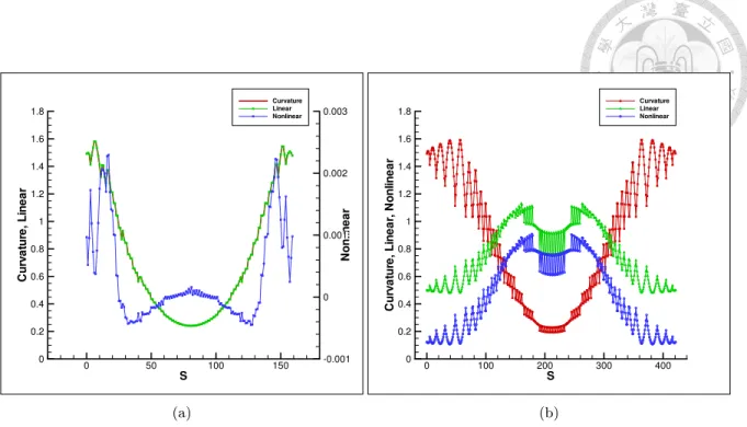
(23) Curvature Linear Nonlinear. 1.8. 0.003. 1.6. 1.4. Curvature, Linear, Nonlinear. 1.6. 0.002. 1.2. Nonlinear. Curvature, Linear. Curvature Linear Nonlinear. 1.8. 1. 0.001 0.8 0.6 0. 0.4 0.2. 1.4 1.2 1 0.8 0.6 0.4 0.2. 0. 0. 50. 100. 150. -0.001. 0. 0. 100. 200. S. S. (a). (b). 300. 400. Figure 8: Plots for indicating the relation among the , N ( ) and r2 along the curve (s) at t = 2.0 for case 1. (a) with reinitialization procedure; (b) without reinitialization procedure. Curvature Weights. 1.8. 0.002. Curvature Weights. 1.8. 1.6. 0.5. 1.6 0.0015. 1.4. 1.4 0.4. Curvature. 0.001 1 0.8. 0.0005 0.6. 1 0.8. 0.3. Weights. 1.2. Weights. Curvature. 1.2. 0.6. 0.4. 0.4. 0. 0.2 0.2 0. 0.2. 0. 50. 100. 150. -0.0005. 0. 0. 100. 200. S. S. (a). (b). 300. 400. Figure 9: Plots for !N along the curve (s) at t = 2.0 for case 1. (a) with reinitialization procedure; (b) without reinitialization procedure. 21.

(24) Curvature Weights. 1 0.8. 1 0.6 0.8. 0.4. Weights. 0.2. Curvature. 0.04. 0. -0.2. 0.2 0.6 0 0.4. -0.2. 0.02. -0.4. -0.4. -0.6. -0.6. 0. 100. 200. 300. 0.2. 0. 0. -0.8. Weights. 0.4. Curvature. 1.2. 0.8. 0.06. 0.6. -1. Curvature Weights. 1. -0.8 -1. 400. 0. 200. 400. S. S. (a). (b). 600. 800. -0.2. Figure 10: Plots for !N along the curve (s) at t = 0.05 for case 3. (a) with reinitialization procedure; (b) without reinitialization procedure. of curves as it is shown in figure 3. To illustrate how reinitialization a↵ects r2 and N ( ) in equation (9), the following two ratios are defined |r2 | |r2 | + |N ( )| |N ( )| !N = 2 |r | + |N ( )| !L =. (33). Figure 7a shows that the ratio !N along the curve with reinitialization procedure being made at t = 1.0. !N is nearly a constant and is close to zero until the curvature approaches zero and becomes negative on (s). Also, the maximum of !N occurs at  = 0. The ratios of the nonlinear terms N ( ) along the curve are all smaller than 0.05. As a result, equation (9) can be regarded as the di↵usion dominated equation with the implementation of reinitialization procedure. Figure 7b shows the evolution of !N without reinitialization at t = 1.0. A very di↵erent relation between  and !N is shown. Starting from the value of 0.2, !N increases its value while curvature decreases. The maximum also occurs at  = 0. Afterwards, !N is rapidly decreased to zero while the curvature of curve keeps decreasing. It is worthy to note here that the relation between !N and curvature  depends on the sign of  in the sense that @ 2 !N < 0 and @2. @!N =0 @. (34) =0. Figure 8a shows that at t = 2.0 the linear source term still dominates the nonlinear term with the reinitialization procedure being applied. The ratio N ( ) is nearly a constant 22.

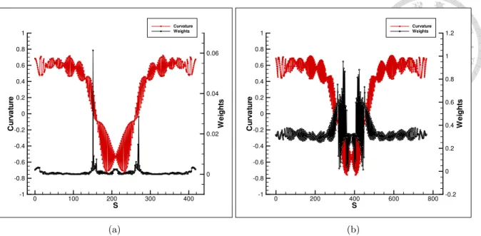
(25) and its value is close to zero along the curve as it is shown in figure 9a. Apparently, the solution for the case without performing reinitialization procedure exhibits oscillatory solution, which indicates the deficiency of WENO scheme. Solutions of , r2 and N ( ) are oscillating along the curve, as it can be seen in figure 8b, while the solutions in figure 8a behave di↵erently. In figure 9b, !N for the solution obtained at t = 2.0 without reinitialization procedure looks similarly to that predicted at t = 1.0. Since N the curvature along the curve at t = 2.0 is positive, !N and  satisfy @! < 0. @. Prediction of a more complex shape of curve helps us to explain the reason of using the combined compact scheme to solve equation (9). Figure 4 shows the motion of the time evolving curve for case 2, which contains a more complicated curvature evolution along the curve. As we mentioned that the motion of the curve is driven by curvature, in physical sense the motion of curve can be considered to be driven by surface tension force. This type of motion has a tendency to reach its minimal surface energy (or minimal surface area), or minimal perimeter in the current two dimensional studies. As it can be seen in figure 4, the curve gradually becomes a circle at t = 0.3. The curve with a complicated evolution and a discontinuity in curvature is then considered for showing the capability of applying the CCD scheme to solve equation (9). Figure 5 shows the evolution of the curve for case 3. In this case, a dramatic change of the curvature is seen along the curve. Note that case 3 is nothing but adding a star-like curve to the two sides of the dumbbell-like curve. Minimal perimeter is reached at both sides of the curve in the beginning of motion and, then, to the whole curve. Figure 10a shows the ratio of nonlinear term N ( ) for the predicted solution without performing reinitialization in case 3 at t = 0.05. The evolution of curve is also dominated by di↵usion, due to the application of reinitialization procedure. The maximum of !N occurs at  = 0, just like that predicted in case 1. Figure 10b exhibits the evolution of !N from the solution without reinitialization and !N and  also satisfy equation (34). Figures 10a and 10b show the solutions with and without reinitialization. Both solutions are oscillatory due to the discontinuous curvature along the curvature. However, while reinitialization procedure is performed, eikonal function |r | = 1 is satisfied, and this results in a smoother solution. It’s worthwhile to note that the curve continuously evolves even the curve has reached its minimal perimeter. By virtue of equation (13), the motion is known to be driven by its local curvature. Since curvature is a positive constant on the perfect circle, the curve keeps shrinking until it becomes a point.. 23.

(26) (a). (b). Figure 11: Task 1. Comparison of the solutions sought at di↵erent times by applying the CCD scheme and the second-order centered di↵erence scheme. The computations are carried out with h = dy = dx = 0.05 and dt = 0.01 ⇥ h. (a) t = 1.0; (b) t = 2.0. In summary, three mean curvature flows have been investigated by using CCD and TVD-RK3 schemes. All the cases under investigation have shown the tendency to reach their minimal perimeter locally or globally. Reinitialization does not a↵ect the motion of curves, but it can redistribute the ratio of the linear and nonlinear terms on the R.H.S. of equation (9). Solutions obtained with reinitialization procedure are strongly a↵ected by the linear source term in equation (9). As a result, mean curvature flow can be regarded as being under the control of pure di↵usion of distance function when reinitialization procedure is applied. Solution obtained without reinitialization procedure is oscillatory in comparison with the smooth solution with reinitialization procedure being performed. The ratio of the nonlinear term increases while the curvature decreases in the region with  > 0. This ratio reaches its maximum at  = 0, and then decreases with the curvature while  < 0. 6.4. Comparison of solutions obtained by CCD and second-order centered schemes. In this section, the reason of applying CCD scheme to predict the motion of curves will be explained through several studies in this subsection. Initially, the shape of the curve is given as p (x x0 )2 + (y y0 )2 = 2.0 + 1.0 cos(!1 ✓) + 0.5 sin(!2 ✓) (35) where ✓ = tan 1 [(y y0 )/(x x0 )]. The degree of complexity of the curve is determined 24.

(27) (a). (b). Figure 12: Task 2. Comparison of the solutions sought at di↵erent times by applying the CCD scheme and the second-order centered di↵erence scheme. The computations are carried out with h = dy = dx = 0.05 and dt = 0.01 ⇥ h. (a) t = 0.0625; (b) t = 0.250. by the coefficients, !1 and !2 . The larger values of !1 and !2 , the larger change of curvatures along the curve. In a box [10,10], the center of the curve is located at (x0 , y0 ) = (5, 5). 6.4.1. Task 1,. (!1 , !2 ) = (0, 0). Investigation of this case is to show that either CCD or second-order centered di↵erence scheme is applicable to disctetize the spatial derivatives. Two solutions remain smooth and are identical with each other. In this task, the choice of !1 = !2 = 0 results in a circle. As it is shown in figure 11, two solutions are identical during the evolution of two curves. Constant curvature is seen along the curve. Both CCD and second-order centered schemes yield accurately simulated evolutions. 6.4.2. Task 2,. (!1 , !2 ) = (5, 6). Another task involves variable curvatures by setting !1 = 5 and !2 = 6 in (35). According to the snap shot of the predicted curve, the solution sought from the second-order centered scheme is more dissipated in the vicinity of the convex and concave parts of the curve. In other words, application of the second-order centered di↵erence scheme yields a smoother solution due to a largely introduced discretization error in the approximation of spatial derivatives. By applying the CCD scheme, one can calculate the curvature term more accurately than that using the second-order centered scheme. As a result, the solution obtained from the CCD scheme is less polluted by the dissipation 25.

(28) (a). (b). Figure 13: Task 3. Comparison of the solutions sought at di↵erent times by applying the CCD scheme and the second-order centered di↵erence scheme. The computations are carried out with h = dy = dx = 0.05 and dt = 0.01 ⇥ h. (a) t = 0.0625; (b) t = 0.250. error introduced to regions with a large curvature, or along the convex and concave parts of the curve. 6.4.3. Task 3,. (!1 , !2 ) = (5, 12). Figure 13 shows the predicted motion of the curve with a more complicated curvature than the curve investigated in task 2. As we mentioned earlier, the solutions obtained from the second-order centered di↵erence scheme are smeared more quickly than CCD scheme does in the sense of introducing more artificial viscosity in the coarse of the simulation of Eq.(9). In summary, it is advantageous to apply the CCD scheme to capture more accurately the motion of curves with less dissipation error being added to the convex and concave parts of curve. Second-order centered di↵erence scheme also provides a good prediction of the motion of curve in case that the curvature does not change rapidly along the curve. If the shape of curve is too complicated, second-order centered di↵erence scheme is not recommended especially in the very beginning phase of the calculation.. 7. Concluding remarks. Within the framework of semi-discretization schemes, an optimal third-order accurate TVD Runge-Kutta temporal scheme for time derivative term and a fifth-order accurate 26.

(29) combined compact di↵erence scheme for spatial derivative terms in the level set equation have been developed in a three-point grid stencil. This computationally efficient finite di↵erence scheme has been applied to simulate mean curvature driven motion of curves, subject to di↵erent initial curves, with great success. Our main objective of this study is to enlighten how two di↵erent mechanisms control the evolution of curve and how they are related to the curvature of the curve under investigation. In the evolution, the surface tension driven curve is subject all the time to the damping e↵ect applied on each point of the curve.. References [1] S. Hildebrandt, H. Karcher (Eds.). Geometric Analytic and Nonlinear Partial Differential Equations. Springer-Verlag Berlin Heidelberg. New York; 2003; ISBN 3540-44051-8. [2] U. Dierkes, S. Hildebrandt, F. Sauvigny. Minimal Surface, Grundlehren der Mathematischen Wissenschaften. Berlin Springer-Verlag; 1992. [3] P. Smereka. Semi-implicit level set methods for curvature and surface di↵usion motion. Journal of Scientific Computing; 2003; 19:439-456. [4] S. Osher, R. P. Fedkiw. Level set methods: An overview and some recent results. Journal of Computational Physics; 2001; 169:463-502. [5] J.A. Sethian. Level Set Methods: Evolving Interfaces in Geometry, Fluid Mechanics, Computer Vision, and Materials Science. Cambridge University Press; 1996. [6] J.A. Sethian, P. Smereka. Level set methods for fluid interface. Ann. Rev. Fluid Mech.; 2003; 35:341-372. [7] D. L. Chopp. Motion by intrinsic Laplacian of curvature. Interfaces and Free Boundary; 1999; 1:107-123. [8] M. Khenner, A. Averbuch, M. Israeli, M. Nathan. Numerical simulation of grainboundary grooving by level set method. Journal of Computational Physics; 2001; 170:764-784. [9] T. Tasdizen, R. Whitaker, P. Burchard, S. Osher. Geometric Surface Processing via Normal Maps. UCLA CAM Report; 2002; 02-03. [10] C. W. Shu, S. Osher. Efficient implementation of essentially non-oscillatory shockcapturing schemes. Journal of Computational Physics; 1968; 77:439-461. 27.

(30) [11] S. Gottlieb, C.W. Shu. Total variation diminishing Runge-Kutta schemes. Mathematics of Computation; 1998; 67:73-85. [12] P. C. Chu., C. Fan. A three point combined compact di↵erence scheme. Journal of Computational Physics; 1998; 140: 370-399. [13] M. Sussman, P. Smereka, S. Osher. A level set approach for computing solutions to incompressible two-phase flow. Journal of Computational Physics; 1994; 114:146159. [14] X. D. Liu, S. Osher, T. Chan. Weighted essential non-oscillatory schemes. Journal of Computational Physics; 1994; 115:200-212. [15] G. S. Jiang, C.W. Shu. Efficient implementation of weighted ENO schemes. Journal of Computational Physics; 1996; 126:202-228. [16] L. T. Cheng, R. Tsai. Redistancing by flow of time dependent eikonal equation. Journal of Computational Physics; 2008; 227:4002-4017. [17] C.W. Shu. High order ENO and WENO schemes for computational fluid dynamics. High-Order Methods for Computational Physics. T.J.Barth and H. Deconinck, editors. Lecture Notes in Computational Science and Engineering. Springer; 1999; 9:439-582. [18] S. Osher, J. A. Sethian. Fronts propagating with curvature-dependent speed: algorithms based on Hamilton-Jacobian formulations. Journal of Computational Physics; 1988; 79:12-49. [19] D. Hartmann, M. Meinke, W. Schroder, Di↵erential equation based constrained reinitialization for level set methods, Journal of Computational Physics; 2008; 227:6821-6845. [20] G. Russo, P. Smereka, A remark on computing distance functions, Journal of Computational Physics; 2000; 163:51-67.. 28.

(31)